Constraints on backreaction in dust universes

Abstract

We study backreaction in dust universes using exact equations which do not rely on perturbation theory, concentrating on theoretical and observational constraints. In particular, we discuss the recent suggestion (in hep-th/0503117) that superhorizon perturbations could explain present-day accelerated expansion as a useful example which can be ruled out. We note that a backreaction explanation of late-time acceleration will have to involve spatial curvature and subhorizon perturbations.

1 Introduction

The idea that averaging inhomogeneous and/or anisotropic spacetimes can lead to behaviour different from the homogeneous and isotropic Friedmann-Robertson-Walker models goes back to at least 1963 [1], and was highlighted as the ’fitting problem’ in 1983 [2]. Under the name backreaction, the effect of inhomogeneities larger than the Hubble scale has been studied in general relativity [3, 4, 5, 6, 7, 8, 9, 10, 11, 12, 13] and in quantized gravity [14], particularly during inflation in the hope that they would provide a graceful exit. It has also been suggested that backreaction from inhomogeneities smaller than the Hubble scale could explain the apparently observed accelerated expansion of the universe today [15, 16], a modern version of the search for a backreaction solution to the age problem in the 1990s [17, 18, 19]. For a useful general formulation of backreaction issues, see [20, 21, 22, 23]. (For a more comprehensive list of backreaction references, see [15, 24].)

Recently it has also been proposed that superhorizon perturbations could explain the late-time acceleration [25, 26, 27, 28]. However, in [29] it was claimed that the effect proposed in [28] amounts only to a renormalisation of the spatial curvature, and is thus severely constrained by observations of the cosmological microwave background and can at any rate never lead to acceleration. There has also been more technical criticism, claiming that a proper accounting of all perturbative terms as well as more general arguments show that the superhorizon modes do not lead to acceleration [30, 31].

We take a viewpoint complementary to that of [30, 31] and study the metric presented in [28] as a concrete example that can used to demonstrate general issues about backreaction in a dust-dominated universe, relevant for both super- and subhorizon perturbations. We will emphasise observational and theoretical constraints and discuss the relation between backreaction and spatial curvature.

In section 2, we examine backreaction using the formalism of [20, 22]. We derive exact bounds on the Hubble parameter and the deceleration parameter. We find that the metric proposed in [28] is ruled out on theoretical grounds if it is valid arbitrarily far into the future, and on observational grounds even if it is to be valid only up until today. If the metric were correct, the effect would not reduce to spatial curvature, though there is a direct link between spatial curvature and backreaction-driven acceleration. In section 3, we discuss general lessons for a backreaction explanation of late-time acceleration, and note that it will have to involve subhorizon perturbations. We then summarise our results and point out the caveats.

2 Constraints on backreaction

2.1 The set-up

The superhorizon backreaction proposal.

In [28] it is assumed that the universe has a homogeneous, isotropic and spatially flat background of dust, and some perturbations denoted by $\Psi(t,\bi{x})$ (but no cosmological constant). The perturbations are divided into two sets of modes, those with wavelengths short and long compared to the Hubble scale, $\Psi(t,\bi{x})=\Psi_{s}(t,\bi{x})+\Psi_{l}(t)$. From the point of view of an observer seeing a single Hubble patch, the spatial dependence of $\Psi_{l}(t)$ is negligible (by definition). The metric in the synchronous gauge is given by

$$ds^{2} = -\rmd t^{2}+a_{FRW}(t)^{2}e^{-2\Psi(t,\bi{x})}\delta_{ij}\rmd x^{i}\rmd x^{j}$$ (1)

$$= -\rmd t^{2}+a_{FRW}(t)^{2}e^{-2\Psi_{s}(t,\bi{x})-2\Psi_{l}(t)}\delta_{ij}\rmd x^{i}\rmd x^{j}$$

$$= -\rmd t^{2}+\left(a_{FRW}(t)e^{-\Psi_{l}(t)}\right)^{2}\delta_{ij}\rmd x^{i}\rmd x^{j}$$

$$\equiv -\rmd t^{2}+a(t)^{2}\delta_{ij}\rmd x^{i}\rmd x^{j}\ ,$$

where $t$ is the proper time measured by a comoving observer, $a_{FRW}(t)=(t/t_{0})^{2/3}$ is the FRW scale factor, the contribution of the short wavelength modes has been neglected, and on the last line we have identified the full scale factor as $a(t)$ (our notation is slightly different from that of [28]). The perturbation is given by $\Psi_{l}(t)=(a_{FRW}(t)-1)\Psi_{l0}$, where the normalisation is $a_{FRW}(t_{0})=1$ and $\Psi_{l}(t_{0})=0$ today. As a function of proper time, the scale factor is then

$$a(t) = e^{\Psi_{l0}}\left(\frac{t}{t_{0}}\right)^{2/3}e^{-\Psi_{l0}(t/t_{0})^{2/3}}\ ,$$ (2)

where the normalisation is $a(t_{0})=1$. The metric (1), (2) is claimed in [28] to be valid to all orders in perturbation theory (a claim analysed in detail in [31]). The departure from FRW behaviour is quantified by $-\Psi_{l0}(t/t_{0})^{2/3}$. If $\Psi_{l0}<0$, backreaction increases the expansion rate and will eventually lead to acceleration. If $|\Psi_{l0}|\sim 1$, the backreaction is relevant already today. The Hubble parameter and the deceleration parameter are

$$H \equiv \frac{\dot{a}}{a}=\frac{2}{3t}(1-\Psi_{l0}(t/t_{0})^{2/3})\equiv\frac{2}{3t}(1+x)$$ (3)

$$q \equiv -\frac{1}{H^{2}}\frac{\ddot{a}}{a}=\frac{1}{2}\frac{1-3x-2x^{2}}{(1+x)^{2}}\ ,$$ (4)

where a dot indicates derivative with respect to the proper time $t$ and we have denoted $x\equiv-\Psi_{l0}(t/t_{0})^{2/3}$. From now on, we assume that $\Psi_{l0}<0$, and thus $x>0$.

The criticism regarding spatial curvature.

In [29], it was argued that the effect discussed in [28] amounts to a simple renormalisation of curvature. The argument is essentially that one can define a new scale factor such that the metric looks like a FRW metric with a curvature term.

This argumentation seems to be incorrect, since for acceleration the relevant issue is the dependence of the scale factor on the proper time, regardless of what notation is used for the scale factor (or proper time). The new scale factor defined in [29] (essentially (2) expanded to first order in $\Psi_{l0}$) still contains a term proportional to $t^{4/3}$ and thus implies acceleration. It is true that the metric involves spatial curvature, but the effect of the perturbations does not reduce to spatial curvature. Nevertheless, the relation between the metric given in (1), (2) and spatial curvature is interesting, and we will take a closer look at it.

The exact average equations.

We follow the formalism for analysing the relation between backreaction and spatial curvature on very general grounds developed in [20] for the dust case (and in [22] for a general ideal fluid). In the present case with only dust, we assume that the vorticity is zero, but otherwise allow for general inhomogeneity and anisotropy. (If vorticity is present, no family of hypersurfaces of constant proper time exists [32, 33], and the formalism of [20, 22] is inapplicable. See also [34].) The Einstein equation then gives the local equations

$$\dot{\theta}+\frac{1}{3}\theta^{2} = -\frac{\kappa^{2}}{2}\rho-2\sigma^{2}$$ (5)

$$\frac{1}{3}\theta^{2} = \kappa^{2}\rho-\frac{1}{2}\mathcal{R}+\sigma^{2}$$ (6)

$$\dot{\rho}+\theta\rho = 0\ ,$$ (7)

where a dot still stands for derivative with respect to the proper time, $\theta(t,\bi{x})$ is the expansion rate of the local volume element, $\kappa^{2}=8\pi G_{N}$ is the gravitational coupling, $\rho(t,\bi{x})$ is the energy density, $\sigma^{2}(t,\bi{x})$ is the shear scalar and $\mathcal{R}(t,\bi{x})$ is the spatial curvature. The energy density and the shear scalar are everywhere non-negative.

Averaging (5), (6) and (7) over a spatial domain (here taken to be the observable universe) with volume $V(t)$, we obtain the equations for the average quantities

$$3\frac{\ddot{a}}{a} = -\frac{\kappa^{2}}{2}\frac{\langle\rho_{0}\rangle}{a^{3}}+\mathcal{Q}$$ (8)

$$3\frac{\dot{a}^{2}}{a^{2}} = \kappa^{2}\frac{\langle\rho_{0}\rangle}{a^{3}}-\frac{1}{2}\langle{\mathcal{R}}\rangle-\frac{1}{2}\mathcal{Q}\ ,$$ (9)

where $a$ is the effective scale factor defined by $a(t)\propto V(t)^{1/3}$, $\rho_{0}$ is the initial value of the energy density and $\langle{A}\rangle$ means the spatial average of the quantity $A$ over the hypersurface of constant proper time $t$,

$$\langle{A}\rangle\equiv\frac{\int d^{3}x\sqrt{{}^{(3)}g}\,A}{\int d^{3}x\sqrt{{}^{(3)}g}}\ ,$$ (10)

where $\sqrt{{}^{(3)}g}$ is the volume element on the hypersurface of constant $t$. Note that $V(t)=\int d^{3}x\sqrt{{}^{(3)}g}$, and $\theta=(\sqrt{{}^{(3)}g})^{-1}\partial_{t}(\sqrt{{}^{(3)}g})$, so $\langle{\theta}\rangle=3\dot{a}/a\equiv 3H$. The backreaction variable $\mathcal{Q}$, defined as

$$\mathcal{Q}\equiv\frac{2}{3}\left(\langle{\theta^{2}}\rangle-\langle{\theta}\rangle^{2}\right)-2\langle{\sigma^{2}}\rangle\ ,$$ (11)

is a qualitatively new term compared to the FRW equations, and embodies the effect of inhomogeneity and anisotropy on the behaviour of the averages.

We emphasise that (8), (9) are exact equations for the averages. There is no need to assume that any perturbations are small, or indeed to have any division into background and perturbations. The equations are general for matter that is a pressureless ideal fluid with zero vorticity.

Note that (8), (9) have the form of FRW equations with effective energy density $\rho_{eff}=\rho-\mathcal{Q}/(2\kappa^{2})$ and effective pressure $p_{eff}=-\mathcal{Q}/(2\kappa^{2})$ [22], though the behaviour of $\langle{\mathcal{R}}\rangle$ and $\mathcal{Q}$ is different from the FRW case. As in the FRW model, the equations (8) and (9) are not independent. The integrability condition is

$$\partial_{t}{\langle{\mathcal{R}}\rangle}+2\frac{\dot{a}}{a}\langle{\mathcal{R}}\rangle=-\dot{\mathcal{Q}}-6\frac{\dot{a}}{a}\mathcal{Q}\ ,$$ (12)

so for $\mathcal{Q}=0$, the equations reduce to the FRW case with $\langle{\mathcal{R}}\rangle\propto a^{-2}$. Likewise, for $\langle{\mathcal{R}}\rangle=0$, backreaction is reduced to the term $\mathcal{Q}\propto a^{-6}$.

The system (8), (9) (or either of them together with (12)) has two equations for the three unknowns $a,\langle{\mathcal{R}}\rangle$ and $\mathcal{Q}$, so it is not closed. This means that different inhomogeneous and/or anisotropic systems sharing the same initial averages can evolve differently even as far as the averages are concerned, as could be expected. It also reflects the fact that sources outside the domain being considered can influence the evolution within the domain. (In the inflationary scenario this does not violate causality even when the domain is the observable universe, since the causally connected region is much larger.)

Given one of the unknowns $a,\langle{\mathcal{R}}\rangle$ and $\mathcal{Q}$, the other two are determined. In particular, the scale factor (2) determines the spatial curvature (and the backreaction variable $\mathcal{Q}$) uniquely regardless of whether (2) originates from long or short wavelength perturbations (or whether the inhomogeneity and/or anisotropy can even be discussed in terms of wave modes). So, we can take the scale factor (2) and plug it into (8), (9) to see what it implies for the spatial curvature (assuming the scale factor results from backreaction, as presented in [28]). However, let us first discuss how it is possible to have accelerated expansion without violating the strong energy condition, and obtain theoretical bounds on the Hubble parameter and acceleration.

2.2 Theoretical constraints

General bounds on $H$ and $q$.

The Raychaudhuri equation (5) shows that the local acceleration is non-positive at each point in spacetime, $\dot{\theta}+\theta^{2}/3\leq 0$. This holds not just for dust, but for any irrotational perfect fluid satisfying the strong energy condition (but does not necessarily hold if vorticity is present). However, the averaged equation (8) does not rule out the possibility that the acceleration $\ddot{a}$ related to the volume is positive. The reason for the apparent discrepancy is that the growth of the volume of the hypersurface of constant proper time compensates for the decrease in the local expansion rate. Technically phrased, averaging and taking the time derivative do not commute: $\partial_{t}\langle{\theta}\rangle=\langle{\dot{\theta}}\rangle+\langle{\theta^{2}}\rangle-\langle{\theta}\rangle^{2}\geq\langle{\dot{\theta}}\rangle$.

Though the acceleration is not limited to be negative, it is possible to derive combined upper limits for the Hubble parameter and the deceleration parameter. Integrating $\dot{\theta}+\theta^{2}/3\leq 0$, we obtain the bound

$$\theta(t,\bi{x})^{-1}-\theta(t_{i},\bi{x})^{-1}\geq\frac{1}{3}(t-t_{i})\ ,$$ (13)

which holds at each point in spacetime; $t_{i}$ is some initial time. This bound has been derived in [35] (and again in [36], where it was applied to the expansion rate of the universe). The inequality (13) is separately valid in domains where $\theta(t,\bi{x})>0$ and in domains where $\theta(t,\bi{x})<0$; it is violated if $\theta(t,\bi{x})$ evolves through zero. Let’s take the initial time to be the big bang time $t_{i}=0$ and assume that $\theta(t_{i},\bi{x})$ is positive. We then have the upper bound $\theta(t,\bi{x})\leq 3/t\equiv\theta_{\textrm{max}}(t)$. This upper bound is also trivially satisfied in domains where $\theta(t,\bi{x})\leq 0$, but there is no limit on the absolute value of $\theta(t,\bi{x})$, corresponding to the fact that the rate of collapse is not bounded from below. Since the average of $\theta$ is at most its maximum value, we obtain an upper bound on the Hubble parameter in terms of the age of the universe:

$$H=\frac{1}{3}\langle{\theta}\rangle\leq\frac{1}{3}\theta_{\textrm{max}}=\frac{1}{t}\ .$$ (14)

The bound (14) implies that the acceleration $\ddot{a}$ cannot increase (or stay constant, if it is positive) forever: it must asymptotically go to zero, become negative or oscillate around zero or a negative value.

We can also put an upper bound on the acceleration as a function of time and the Hubble parameter. The averaged Raychaudhuri equation (8) implies that

$$q=-\frac{1}{H^{2}}\frac{\ddot{a}}{a}\geq 2-\frac{2}{9}\frac{\langle{\theta^{2}}\rangle}{H^{2}}\geq 2-\frac{2}{9}\frac{(\theta_{\textrm{max}})^{2}}{H^{2}}=2-2\frac{1}{(Ht)^{2}}\ .$$ (15)

In the second inequality we have assumed that $\langle{\theta^{2}}\rangle\leq(\theta_{\textrm{max}})^{2}$, which is not necessarily true if $\theta$ is somewhere negative. This the case in regions of the universe which are undergoing gravitational collapse. However, the expansion rate of the universe is generally understood to measure expansion between regions which have collapsed, so it is not clear whether the insides of such regions should be included in the averaging. (According to the inequality $\dot{\theta}+\theta^{2}/3\leq 0$, once a region starts collapsing, the collapse rate can only increase. In order for the region to virialise and stabilise, vorticity or a breakdown in the approximation of treating the matter as dust [37] is required, so in the present calculation collapsing regions cannot be treated properly anyway.)

Bounds on the superhorizon proposal.

The bounds (14) and (15) are valid for any model where the matter is (irrotational) dust (with a caveat about the positivity of the expansion rate for the latter bound). In particular, these bounds can be applied to the metric presented in [28]. The scale factor (2) is $a\propto xe^{x}$, where $x=|\Psi_{l0}|(t/t_{0})^{2/3}$, so $\ddot{a}$ will increase forever and the metric is ruled out. In more detail, with the expansion rate and the deceleration parameter given by (3) and (4), the theoretical bounds (14) and (15) reduce to $x\leq 1/2$ and $x\leq(\sqrt{265}-11)/12\approx 0.44$, respectively. Since $x=|\Psi_{l0}|(t/t_{0})^{2/3}$ grows without bound, these bounds will necessarily be violated at some point: backreaction in a dust universe (without rotation) cannot produce the scale factor (2), if it is taken to be valid arbitrarily far into the future. However, it could still be that the metric is only valid as an approximation up until today, and the acceleration would slow down in the future so as to respect the bounds (14), (15). Assuming the scale factor (2) to be valid till today, we get the bound $|\Psi_{l0}|\leq(\sqrt{265}-11)/12\approx 0.44$. Let us now look at observational constraints on the metric in light of the evolution given by (8), (9) and compare to this theoretical bound.

2.3 Observational constraints

Evolution of the density parameters.

We have noted that the local acceleration is everywhere non-positive, while the acceleration related to the total volume may be positive. This raises the question of which is the correct quantity to consider. The answer depends on what observations one is comparing to. More generally, there are several different measures of the expansion rate and acceleration. For example, number counts (and thus the energy density of dust) depend on $\theta$ which gives the volume, luminosity distances depend on different parameters [27, 30, 31], the rate of change in the distance $\delta l$ between neighbouring fluid lines $\dot{\delta l}/\delta l$ is yet another observable given by $\theta/3+\sigma_{\alpha\beta}n^{\alpha}n^{\beta}$, with $\sigma_{\alpha\beta}$ being the shear tensor and $n^{\alpha}$ the unit separation vector between the fluid lines [33]. These measures coincide in the homogeneous and isotropic FRW case, but in general they give different results for inhomogeneous and/or anisotropic models, so one should be careful to consider the quantities that are actually being observed (in the case of acceleration, luminosity distances of type Ia supernovae). Conversely, agreement between different measures can be one way to constrain the possibility that backreaction is responsible for the apparently observed acceleration.

We will not discuss these issues further, but will simply assume, following [28], that measures of the expansion rate and acceleration are related to the scale factor and its derivatives in the same way as in FRW models. We will take the scale factor $a(t)\propto V(t)^{1/3}$ to be given by (2), proposed to arise from backreaction in [28], and study the observational implications. As noted earlier, we treat the metric of [28] as an interesting example with which to look at backreaction. The predictions of any future backreaction models for $a(t)$ could be analysed in the same manner. Given the scale factor (2), equations (8) and (9) yield the quantities $\langle{\mathcal{R}}\rangle$ and $\mathcal{Q}$ as

$$\langle{\mathcal{R}}\rangle = -\frac{2}{3t^{2}}\left(3-3e^{-3x}+11x+6x^{2}\right)$$

$$\mathcal{Q} = \frac{2}{3t^{2}}\left(e^{-3x}-1+3x+2x^{2}\right)\ ,$$ (16)

where, as before, $x=|\Psi_{l0}|(t/t_{0})^{2/3}$. The spatial curvature is negative, $\langle{\mathcal{R}}\rangle<0$, so the universe is open.

The relative contributions of dust, spatial curvature and the backreaction variable $\mathcal{Q}$ to the expansion rate can be discussed in analogy with the FRW case in terms of the relative densities [20, 23]

$$\Omega_{m} \equiv \frac{\kappa^{2}\langle\rho_{0}\rangle a^{-3}}{3H^{2}}=\frac{e^{-3x}}{(1+x)^{2}}$$

$$\Omega_{\mathcal{R}} \equiv -\frac{\langle{\mathcal{R}}\rangle}{6H^{2}}=\frac{1}{4}\frac{3-3e^{-3x}+11x+6x^{2}}{(1+x)^{2}}$$

$$\Omega_{\mathcal{Q}} \equiv -\frac{\mathcal{Q}}{6H^{2}}=-\frac{1}{4}\frac{e^{-3x}-1+3x+2x^{2}}{(1+x)^{2}}\ ,$$ (17)

so that $\Omega_{m}+\Omega_{\mathcal{R}}+\Omega_{\mathcal{Q}}=1$. As discussed in [20, 21, 23, 38], backreaction is not important just because $\Omega_{\mathcal{Q}}$ can be large, but also because the presence of a new term changes the behaviour of the spatial curvature from the FRW case, as shown by (12).

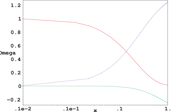
(a)

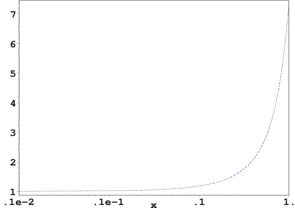
(b)

Figure 1: The behaviour of the components as a function of $x=|\Psi_{l0}|(t/t_{0})^{2/3}$. (a): The relative densities of matter, spatial curvature and the backreaction variable $\mathcal{Q}$. Red (solid) is $\Omega_{m}$, blue (dash-dot) is $\Omega_{\mathcal{R}}$ and green (dash) is $\Omega_{\mathcal{Q}}$. (b): The spatial curvature $\langle{\mathcal{R}}\rangle a^{2}$ relative to its asymptotic past value.

The density parameters are plotted in figure 1(a). At early times, until $x\approx 10^{-2}$, the behaviour is the same as in the FRW case, with the matter density being dominant (as is clear from the Hubble law (3)). At late times, the expansion accelerates, the matter density becomes negligible, and the contributions of the spatial curvature and the backreaction variable approach the limiting values $\Omega_{\mathcal{R}}=3/2$ and $\Omega_{\mathcal{Q}}=-1/2$. Asymptotically, the expansion is driven by the spatial curvature $\langle{\mathcal{R}}\rangle=-9H^{2}$ and the backreaction variable $\mathcal{Q}=3H^{2}$. Note that the behaviour can differ significantly from the FRW case even when the contribution of the backreaction variable $\Omega_{\mathcal{Q}}$ is numerically small. For example, for $x=0.1$, we have $\Omega_{\mathcal{Q}}\approx-0.01$, but the contribution of matter has fallen to $\Omega_{m}\approx 0.61$.

Comparing to observations.

The Hubble parameter, spatial curvature and other relevant quantities today are determined by the single free parameter $|\Psi_{l0}|$ (along with the age of the universe). We will constrain $|\Psi_{l0}|$ by looking at the observed values of the Hubble parameter and the deceleration parameter today, combined with the age of the universe. From (3) and (4), we have

$$H_{0} = \frac{2}{3t_{0}}(1+|\Psi_{l0}|)$$ (18)

$$q_{0} = \frac{1}{2}\frac{1-3|\Psi_{l0}|-2|\Psi_{l0}|^{2}}{(1+|\Psi_{l0}|)^{2}}\ .$$ (19)

Leaving aside the issue that observations might need to be reanalysed in the context of a backreaction model (as mentioned above), as well as possible unaccounted systematics in the determination of the Hubble parameter [39], we take $H_{0}=h$ 100 km/s/Mpc $=72\pm 8$ km/s/Mpc, giving $h$ between 0.56 and 0.88 [40]. The expression (18) can be written as $1+|\Psi_{l0}|\approx 2.0h\times t_{0}/(13\textrm{ billion years})$. Putting the upper limit on $h$ together with the requirement that the universe is at most 15 billion years old gives (disregarding correlation in the observational values of $H_{0}$ and age) the limit $|\Psi_{l0}|\lesssim 1.0$. On the other hand, the constraint $q_{0}\lesssim-0.3$ [41] applied to (19) gives $|\Psi_{l0}|\gtrsim 0.60$. With (18), this limit can be written as $h\gtrsim 0.80/(t_{0}/$13 billion years).

There is some tension between the age and acceleration constraints: having enough acceleration requires a large $|\Psi_{l0}|$, which boosts $H_{0}$, so $t_{0}$ needs to be large to bring $H_{0}$ down in line with the observations. This is related to the fact that the transition from the FRW dust behaviour to acceleration is smoother than in $\Lambda$CDM: the scale factor (2) corresponds to the behaviour of a FRW model with dust replaced by a fluid with the equation of state $-x/(1+x)$, and two added fluids having the equations of state $-(1+3x)/(3+3x)$ and $-(2+3x)/(3+3x)$. The tension is not significant, but we have mentioned it to show what kind of an impact the age and acceleration constraints have on backreaction ideas, in particular in relation to the sharpness of the transition to acceleration. Obviously, this issue is the same as in models of dark energy. For a more thorough analysis of sharp transition into acceleration in light of SNIa and other cosmological data, see [42].

For $|\Psi_{l0}|=0.60$ we have $\Omega_{m0}=0.06$, $\Omega_{\mathcal{R}0}=1.10$ and $\Omega_{\mathcal{Q}0}=-0.16$. The universe is dominated by curvature, with subdominant contributions from the backreaction variable and matter. Leaving the small matter density aside, it might seem that the model is straightforwardly ruled out by constraints on the spatial curvature from the CMB in models with adiabatic perturbations (the constraints in the case with correlated adiabatic and isocurvature perturbations are unknown).

However, when backreaction effects are important the spatial curvature behaves (at least in a dust universe) quite differently from the FRW case. In figure 1(b) we have plotted the quantity $\langle{\mathcal{R}}\rangle a^{2}$, which is constant in FRW models. The spatial curvature rises faster than in the FRW case, so it will have less impact in the past. However, the suppression factor is not large (about 0.32 for $|\Psi_{l0}|=0.60$), and though the observations would need to be reanalysed with the full inhomogeneous metric, it seems unlikely that the spatial curvature would be compatible with the CMB data (at least with adiabatic perturbations).

These observational constraints on the scale factor (2) are independent from the theoretical constraints discussed earlier. In terms of $h$, the theoretical bounds (14), (15) give

$$h\times t_{0}/(13\textrm{ billion years})\lesssim 0.75$$ (20)

$$q_{0}\gtrsim 2-\frac{1.13}{(h\times t_{0}/(13\textrm{ billion years}))^{2}}\ .$$ (21)

The limit $h\times t_{0}/(13\textrm{ billion years})\gtrsim 0.80$ that we obtained previously by comparing the scale factor (2) to observations of $q_{0}$ is in contradiction with (20). Applied to (21), the limit on $h$ implies $q_{0}\gtrsim 0.23$, which is even more clearly inconsistent. So, the observational lower limit $|\Psi_{l0}|\gtrsim 0.60$ is strongly contradicted by the theoretical upper bound $|\Psi_{l0}|\lesssim 0.44$. This means that backreaction cannot produce the scale factor (2), even as an approximation valid only up until today. In physical terms, the slow onset of acceleration in (2) means that to match the observations, the universe has to be far in the regime where backreaction is important, which in turn makes the Hubble parameter higher than irrotational inhomogeneity or anisotropy in dust can produce.

The bounds (20), (21) can be used together with observations to constrain backreaction ideas in general. In practice, (21) gives the more stringent constraint: the limit $q_{0}\lesssim-0.3$ gives $h\times t_{0}/(13\textrm{ billion years})\lesssim 0.70$. This bound is below the current observational central value: there is no contradiction at present, but future observations may be able to show that the bound is violated. This would mean that a backreaction explanation for the observed acceleration is ruled out (with caveats about vorticity, positivity of the expansion rate and the interpretation of observations).

3 Discussion

Lessons for backreaction.

The analysis of the metric (1), (2) has allowed us to look at general features of backreaction in a dust-dominated universe (some brought up already in [20, 21, 38]) in a quantitative manner.

The backreaction variable $\mathcal{Q}$ contributes positively to the acceleration (8), but negatively to the square of the Hubble parameter (9). If backreaction increases the expansion rate, this can only be consistent if there is a compensating spatial curvature so that $|\langle{\mathcal{R}}\rangle|>\mathcal{Q}$ and $\langle{\mathcal{R}}\rangle<0$. Significant backreaction implies significant spatial curvature. The fact that spatial curvature is integral to backreaction does not mean that backreaction as a source of late-time acceleration is ruled out, since the behaviour of spatial curvature is different from the FRW case. The CMB data would need to be analysed with the particular inhomogeneous metric leading to backreaction, not just the averaged equations. (Note that since the spatial curvature is time-dependent, perturbations cannot be expanded in terms of Fourier modes or the basis functions for other spaces of constant curvature.) But it seems likely that in order for the spatial curvature not to conflict with observations, it should decrease rapidly towards the past. (Note that negative spatial curvature boosts the amplitudes of the low multipoles of the CMB via the Integrated Sachs-Wolfe effect. In general, spatial curvature leads to a stronger ISW effect than a cosmological constant with the same relative density, since spatial curvature is important for a longer period of time, so a transition that is more rapid than in the $\Lambda$CDM model could yield a smaller ISW effect.)

In other words, in order for a backreaction explanation to be viable, the transition from standard FRW behaviour to acceleration would need to be sharper than in the scale factor (2). This is also suggested by the tension between the observational age and acceleration constraints. A sharp transition would sit well with the idea of backreaction from small wavelength modes related to structure formation: the expansion rate would be the FRW one until structure formation becomes important, and then change rapidly. (Backreaction from structure formation would also present a solution to the coincidence problem, unlike backreaction from superhorizon modes.)

Note that according to (8) and (11) accelerated expansion requires a variance of the expansion rate of order unity. Though we have simply assumed that superhorizon modes lead to the scale factor (2), it in fact implies significant subhorizon perturbations (if it arises from backreaction). This shows that, observational constraints aside, superhorizon perturbations alone cannot lead to late-time acceleration.

The relation between variance and backreaction is in agreement with the suggestion made in [15] (and borne out in [43] for the Lemaître-Tolman-Bondi model) that the Weyl tensor could provide a measure of backreaction. On the other hand, large backreaction from highly isotropic long-wavelength modes as in [28] (which presumably do not contribute much to the Weyl tensor) would contradict this idea.

Let us also note that the isotropy of the CMB would naively seem to rule out variations larger than $10^{-5}$ in the expansion rate in different directions, and it seems unclear how this could be reconciled with the large variance needed for backreaction to produce acceleration. However, the link between geometric inhomogeneity and/or anisotropy and the isotropy of the CMB is not straightforward, and it is not clear that such a large variance is ruled out either. For example, it is possible for a spacetime to be very anisotropic even though the CMB looks almost isotropic [44]. See [34, 45] for a careful analysis of the limits the isotropy of the CMB places on the spatial variation of the expansion rate and related quantities, and [46] for further discussion and counter-examples. For another point of view, note that the difference in the expansion rate between expanding regions and regions which have broken away from the expansion and collapsed is indeed of order one, without contradicting the isotropy of the CMB.

A possible way of avoiding the large variance would be that backreaction does not lead to acceleration as measured by the volume expansion $\theta$, but does give real or apparent acceleration according to other measures, for example the luminosity distance (along the lines of [27]). In fact, it has been claimed that cluster counts (which depend on $\theta$ more directly than SNIa luminosity distances) are consistent with deceleration and inconsistent with acceleration [47].

Conclusion.

We have looked at constraints on backreaction-driven acceleration in a dust-dominated universe, applying the exact formalism for backreaction developed in [20]. In particular, we have analysed the model for late-time acceleration presented in [28] as a useful example, with emphasis on theoretical and observational constraints as well as spatial curvature, which was claimed in [29] to explain away the effect.

We have derived exact bounds for the expansion rate and acceleration, valid for any models where the matter is irrotational dust. In particular, acceleration cannot increase forever. This rules out the metric proposed in [28] on theoretical grounds, if it is to be valid arbitrarily far into the future. We also have also shown that, when supplemented with observational bounds on the Hubble parameter or the deceleration parameter, the theoretical bounds rule out the metric proposed in [28] even as an approximation valid only up until today.

If the scale factor in [28] were correct, we find that the backreaction would not reduce to spatial curvature, and the universe would accelerate. However, growth of spatial curvature is an integral part of backreaction leading to acceleration, and the slow transition into acceleration in [28] implies that curvature is important for a long period, which is probably not compatible with the CMB data. The same conclusion applies to any model aiming to explain late-time acceleration with backreaction, whether from superhorizon modes or inhomogeneities related to structure formation. This suggests that for backreaction to be a possible explanation, the transition from standard FRW behaviour to acceleration should be rapid. Acceleration from backreaction also implies that the variance of the expansion rate within the observable universe is large, showing that superhorizon perturbations alone cannot be responsible (which is the case in [28]).

The analysis does not depend on any assumptions regarding the amplitude and wavelength of the inhomogeneities and/or anisotropies. However, it is assumed that the cosmic fluid is completely pressureless, ideal (for example, has no viscosity) and irrotational. Possibilities for avoiding the growth of spatial curvature thus include the presence of vorticity (as mentioned in [31]), or a breakdown in the approximation of treating the cosmic matter as a pressureless ideal fluid, as conjectured in [48] (see also [37]). Another possibility is that instead of giving acceleration, backreaction would change the interpretation of observations so that they are consistent with decelerating expansion.

The above arguments do not apply to backreaction during inflation in the early universe driven by the cosmological constant or a scalar field. However, a single scalar field can be described in terms of an ideal fluid, and it would be interesting to extend the analysis to backreaction in single field inflation, as suggested in [22].

Finally, let us note that even though the proposal in [28] of backreaction from superhorizon modes is not correct, it provides a useful example of a backreaction model which it is possible to analytically discuss. It is more difficult to calculate the backreaction of small wavelength modes, but it would be helpful to find some, perhaps simplified, model to concretely demonstrate the general issues discussed here in the context of subhorizon perturbations.

References

- [1] Shirokov M F and Fisher I Z, Isotropic Space with Discrete Gravitational-Field Sources. On the Theory of a Nonhomogeneous Universe, 1963 Sov. Astron. J. 6 699 Reprinted in Gen. Rel. Grav. 30 1411, 1998
- [2] Ellis G F R, Relativistic cosmology: its nature, aims and problems, 1983 The invited papers of the 10th international conference on general relativity and gravitation, p 215 Ellis G F R and Stoeger W, The ’fitting problem’ in cosmology, 1987 Class. Quant. Grav. 4 1697
- [3] Mukhanov V F, Abramo L R W and Brandenberger R H, Back Reaction Problem for Gravitational Perturbations, 1997 Phys. Rev. Lett. 78 1624 [gr-qc/9609026] Abramo L R W, Brandenberger R H and Mukhanov V F, The Energy-Momentum Tensor for Cosmological Perturbations, 1997 Phys. Rev. D56 3248 [gr-qc/9704037]
- [4] Unruh W, Cosmological long wavelength perturbations [astro-ph/9802323]
- [5] Geshnizjani G and Brandenberger R, Back Reaction And Local Cosmological Expansion Rate, 2002 Phys. Rev. D66 123507 [gr-qc/0204074]
- [6] Brandenberger R H, Back Reaction of Cosmological Perturbations and the Cosmological Constant Problem [hep-th/0210165]
- [7] Finelli F, Marozzi G, Vacca G P and Venturi G, Energy-Momentum Tensor of Cosmological Fluctuations during Inflation, 2004 Phys. Rev. D69 123508 [gr-qc/0310086]
- [8] Geshnizjani G and Brandenberger R, Back Reaction Of Perturbations In Two Scalar Field Inflationary Models, 2005 JCAP0504(2005)006 [hep-th/0310265]
- [9] Brandenberger R and Mazumdar A, Dynamical Relaxation of the Cosmological Constant and Matter Creation in the Universe, 2004 JCAP0408(2004)015 [hep-th/0402205]
- [10] Geshnizjani G and Afshordi N, Coarse-Grained Back Reaction in Single Scalar Field Driven Inflation, 2005 JCAP0501(2005)011 [gr-qc/0405117]
- [11] Brandenberger R H and Lam C S, Back-Reaction of Cosmological Perturbations in the Infinite Wavelength Approximation [hep-th/0407048]
- [12] Brandenberger R H and Martin J, Back-reaction and the trans-Planckian problem of inflation revisited, 2005 Phys. Rev. D71 023504 [hep-th/0410223]
- [13] Nambu Y, The separate universe and the back reaction of long wavelength fluctuations, 2005 Phys. Rev. D71 084016 [gr-qc/0503111]
- [14] Tsamis N C and Woodard R P, Quantum Gravity Slows Inflation, 1996 Nucl. Phys. B474 235 [hep-ph/9602315] Tsamis N C and Woodard R P, The Quantum Gravitational Back-Reaction on Inflation, 1997 Annals Phys. 253 1 [hep-ph/9602316] Abramo L R, Tsamis N C and Woodard R P, Cosmological Density Perturbations From A Quantum Gravitational Model Of Inflation, 1999 Fortsch. Phys. 47 389 [astro-ph/9803172] Woodard R P, Effective Field Equations of the Quantum Gravitational Back-Reaction on Inflation [astro-ph/0111462] Woodard R P, A leading logarithm approximation for inflationary quantum field theory, [astro-ph/0502556]
- [15] Räsänen S, Dark energy from backreaction, 2004 JCAP0402(2004)003 [astro-ph/0311257] Räsänen S, Backreaction of linear perturbations and dark energy [astro-ph/0407317]
- [16] Notari A, Late time failure of Friedmann equation [astro-ph/0503715]
- [17] Bildhauer S and Futamase T, The Age Problem in Inhomogeneous Universes, 1991 Gen. Rel. Grav. 23 1251
- [18] Russ H, Soffel M H, Kasai M and Börner G, Age of the Universe: Influence of the Inhomogeneities on the global Expansion-Factor, 1997 Phys. Rev. D56 2044 [astro-ph/9612218]
- [19] Sicka C, Buchert T and Kerscher M, Backreaction in cosmological models [astro-ph/9907137]
- [20] Buchert T, On average properties of inhomogeneous fluids in general relativity I: dust cosmologies, 2000 Gen. Rel. Grav. 32 105 [gr-qc/9906015]
- [21] Buchert T, On average properties of inhomogeneous cosmologies, 2000 Proceedings of the 9th JGRG meeting, p 306 [gr-qc/0001056]
- [22] Buchert T, On average properties of inhomogeneous fluids in general relativity II: perfect fluid cosmologies, 2001 Gen. Rel. Grav. 33 1381 [gr-qc/0102049]
- [23] Buchert T and Carfora M, The Cosmic Quartet - Cosmological Parameters of a Smoothed Inhomogeneous Spacetime [astro-ph/0312621]
- [24] Krasiński A, Inhomogeneous Cosmological Models, 1997 Cambridge University Press, Cambridge
- [25] Kolb E W, Matarrese S, Notari A and Riotto A, The effect of inhomogeneities on the expansion rate of the universe, 2005 Phys. Rev. D71 023524 [hep-ph/0409038]
- [26] Kolb E W, Matarrese S, Notari A and Riotto A, Cosmological influence of super-Hubble perturbations, 2005 Mod. Phys. Lett. A20 2705 [astro-ph/0410541]
- [27] Barausse E, Matarrese S and Riotto A, The Effect of Inhomogeneities on the Luminosity Distance-Redshift Relation: is Dark Energy Necessary in a Perturbed Universe?, 2005 Phys. Rev. D71 063537 [astro-ph/0501152]
- [28] Kolb E W, Matarrese S, Notari A and Riotto A, Primordial inflation explains why the universe is accelerating today [hep-th/0503117]
- [29] Geshnizjani G, Chung D J H and Afshordi N, Do Large-Scale Inhomogeneities Explain Away Dark Energy?, 2005 Phys. Rev. D72 023517 [astro-ph/0503553]
- [30] Flanagan E E, Can superhorizon perturbations drive the acceleration of the Universe?, 2005 Phys. Rev. D71 103521 [hep-th/0503202]
- [31] Hirata C M and Seljak U, Can superhorizon cosmological perturbations explain the acceleration of the universe?, 2005 Phys. Rev. D72 083501 [astro-ph/0503582]
- [32] Ehlers J, Contributions to the relativistic mechanics of continuous media, 1993 Gen. Rel. Grav. 25 1225 (Originally 1961, Abh. Akad. Wiss. Lit. Mainz. Nat. Kl. 11 793)
- [33] Raychaudhuri A K, An Approach To Anisotropic Cosmologies, 1989 Gravitation, gauge theories and the early universe, ed Iyer B R et al Kluwer, Dordrecht p 89
- [34] Stoeger W R, Maartens R and Ellis G F R, Proving almost homogeneity of the universe: An Almost Ehlers-Geren-Sachs theorem, 1995 Astrophys. J. 443 1
- [35] Wald R M, General Relativity, 1984 The University of Chicago Press, Chicago p 220
- [36] Nakamura T, Nakao K-i, Chiba T and Shiromizu T, Volume expansion rate and age of universe, 1995 Mon. Not. Roy. Astron. Soc. 276 L41 [astro-ph/9507085]
- [37] Buchert T and Domínguez A, Adhesive Gravitational Clustering, 2005 Astron. & Astrophys. 438 443 [astro-ph/0502318]
- [38] Buchert T, Kerscher M and Sicka C, Backreaction of inhomogeneities on the expansion: the evolution of cosmological parameters, 2000 Phys. Rev. D62 043525 [astro-ph/9912347]
- [39] Blanchard A, Douspis M, Rowan-Robinson M and Sarkar S, An alternative to the cosmological ’concordance model’, 2003 Astron. & Astrophys. 412 35 [astro-ph/0304237] Sarkar S, Measuring the cosmological density perturbation, 2005 Nucl. Phys. B Proc. Suppl. 148 1 [hep-ph/0503271]
- [40] Freedman W L et al, Final Results from the Hubble Space Telescope Key Project to Measure the Hubble Constant, 2001 Astrophys. J. 553 47 [astro-ph/0012376]
- [41] Riess A G et al(Supernova Search Team Collaboration), Type Ia Supernova Discoveries at From the Hubble Space Telescope: Evidence for Past Deceleration and Constraints on Dark Energy Evolution, 2004 Astrophys. J. 607 665 [astro-ph/0402512]
- [42] Bassett B A, Kunz M, Silk J and Ungarelli C, A late-time transition in the cosmic dark energy?, 2002 Mon. Not. Roy. Astron. Soc. 336 1217 [astro-ph/0203383] Alam U, Sahni V and Starobinsky A A, Is there Supernova Evidence for Dark Energy Metamorphosis?, 2004 Mon. Not. Roy. Astron. Soc. 354 275 [astro-ph/0311364] Alam U, Sahni V and Starobinsky A A, The case for dynamical dark energy revisited, 2004 JCAP0406(2004)008 [astro-ph/0403687] Jonsson J, Goobar A, Amanullah R and Bergstrom L, No evidence for Dark Energy Metamorphosis?, 2004 JCAP09(2004)007 [astro-ph/0404468] Corasaniti P S, Kunz M, Parkinson D, Copeland E J and Bassett B A, The foundations of observing dark energy dynamics with the Wilkinson Microwave Anisotropy Probe, 2004 Phys. Rev. D70 083006 [astro-ph/0406608] Alam U, Sahni V and Starobinsky A A, Rejoinder to No Evidence of Dark Energy Metamorphosis [astro-ph/0406672] Hannestad S and Mörtsell E, Cosmological constraints on the dark energy equation of state and its evolution, 2004 JCAP0409(2004)001 [astro-ph/0407259] Bassett B A, Corasaniti P S and Kunz M, The essence of quintessence and the cost of compression, 2004 Astrophys. J. 617 L1 [astro-ph/0407364]
- [43] Räsänen S, Backreaction in the Lemaître-Tolman-Bondi model, 2004 JCAP0411(2004)010 [gr-qc/0408097]
- [44] Wainwright J, Hancock M J and Uggla C, Asymptotic self-similarity breaking at late times in cosmology, 1999 Class. Quant. Grav. 16 2577 [gr-qc/9812010] Nilsson U S, Uggla C, Wainwright J and Lim W C, An almost isotropic cosmic microwave temperature does not imply an almost isotropic universe, 1999 Astrophys. J. 522 L1 [astro-ph/9904252] Lim W C, Nilsson U S and Wainwright J, Anisotropic universes with isotropic cosmic microwave background radiation, 2001 Class. Quant. Grav. 18 5583 [gr-qc/9912001]
- [45] Maartens R, Ellis G F R and Stoeger W R, Limits on anisotropy and inhomogeneity from the cosmic background radiation, 1995 Phys. Rev. D51 1525 [astro-ph/9501016] Maartens R, Ellis G F R and Stoeger W R, Improved limits on anisotropy and inhomogeneity from the cosmic background radiation, 1995 Phys. Rev. D51 5942 Maartens R, Ellis G F R and Stoeger W R, Anisotropy and inhomogeneity of the universe from , 1996 Astron. & Astrophys. 309 L7 [astro-ph/9510126] Stoeger W R, Araujo M and Gebbie T, The Limits on Cosmological Anisotropies and Inhomogeneities from COBE Data, 1997 Astrophys. J. 476 435 [astro-ph/9904346]
- [46] Clarkson C A and Barrett R K, Does the Isotropy of the CMB Imply a Homogeneous Universe? Some Generalised EGS Theorems, 1999 Class. Quant. Grav. 16 3781 [gr-qc/9906097] Barrett R K and Clarkson C A, Undermining the Cosmological Principle: Almost Isotropic Observations in Inhomogeneous Cosmologies, 2000 Class. Quant. Grav. 17 5047 [astro-ph/9911235] Clarkson C A, Coley A A, O’Neill E S D, Sussman R A and Barrett R K, Inhomogeneous cosmologies, the Copernican principle and the cosmic microwave background: More on the EGS theorem, 2003 Gen. Rel. Grav. 35 969 [gr-qc/0302068]
- [47] Vauclair S C et al, The XMM–NEWTON Omega Project: II. Cosmological implications from the high redshift L-T relation of X-ray clusters, 2003 Astron. & Astrophys. 412 L37 [astro-ph/0311381] Blanchard A, Cosmological Interpretation from High Redshift Clusters Observed Within the XMM-Newton -Project [astro-ph/0502220]
- [48] Schwarz D J, Accelerated expansion without dark energy, [astro-ph/0209584]