Galactic Wind Effects on the Ly$\alpha$ Absorption in the Vicinity of Galaxies

Abstract

We present predictions of Ly$\alpha$ forest-galaxy correlations at $z=3$ from Eulerian simulations that include the effects of galactic winds, driven primarily by supernova explosions. Galactic winds produce expanding bubbles of shock-heated gas within $\sim 0.5$ comoving $\,h^{-1}\;{\rm Mpc}$ of luminous galaxies in the simulation, which have space density similar to that of observed Lyman break galaxies (LBGs). However, most of the low-density intergalactic gas that determines the observed properties of the Ly$\alpha$ forest is unaffected by winds. The impact of winds on the Ly$\alpha$ optical depth near galaxies is less dramatic than their impact on gas temperature because winds heat only a small fraction of the gas present in the turnaround regions surrounding galaxies. Hence, Ly$\alpha$ absorption from gas outside the wind bubbles is spread out over the same velocity range occupied by the wind-heated gas. In general, Ly$\alpha$ absorption is expected to be stronger than average near galaxies because of the high gas density. Winds result in a modest reduction of this expected increase of Ly$\alpha$ absorption. Our predictions can be compared to future observations to detect the wind effects and infer their strength, although with the caveat that the results are still dependent on the correspondence of simulated galaxies and observed LBGs. We find that wind effects in our simulations are not strong enough to reproduce the high Ly$\alpha$ transmission within 0.5 $\,h^{-1}\;{\rm Mpc}$ comoving of galaxies that has been suggested by recent observations; powerful galactic explosions or ejecta with hyper-escape velocities would be required, but these are unlikely to be produced by ordinary star formation and supernovae alone.

1 Introduction

Galactic winds are an important but poorly understood aspect of galaxy formation and evolution. Winds are observed locally (e.g., Heckman et al. 1998; Martin 1998), but are probably more important at high redshift where star formation and the subsequent supernovae occur at the fastest rate. Winds have been invoked as an important force for forming galaxies (Ostriker & Cowie, 1981), and more recently their effects have been proposed as a solution to various problems related to galaxy formation, from the suppression of star formation in low mass halos (now the dark dwarf satellites predicted to orbit galaxies like the Milky Way; e.g., Dekel & Silk 1986), to the metal pollution of the intergalactic medium (hereafter, IGM; see, e.g., Aguirre et al. 2001). Luminous, star-forming galaxies at high redshift, or Lyman break galaxies (hereafter, LBGs) show evidence of outflows in their spectra (Pettini et al., 2002) with velocities of up to 1000 $\,{\rm km}\;{\rm s}^{-1}$.

Such outflows may not only affect star formation within the galaxy, but may potentially impact the surrounding intergalactic gas as well. Recently, Adelberger et al. (2003) have reported a “galaxy proximity effect” in the IGM around LBGs. The effect consists of an increase in the Ly$\alpha$ transmitted flux within a comoving transverse separation of $\sim 1\,h^{-1}\;{\rm Mpc}$ and at the redshift of the LBG as measured on a parallel line of sight probed by a quasar. This is contrary to the expected decrease of transmitted flux (or increased absorption) owing to increased gas density in the vicinity of a galaxy predicted by the gravitational instability model, which has been observed at low redshift (e.g., Morris et al. 1993; Lanzetta et al. 1995; Chen et al. 1998). Adelberger et al. (2003) interpreted their observations as indicating the effects of galactic super-winds that would have either swept up the absorbing gas, or otherwise heated it sufficiently to remove its absorption signature entirely.

The strength of a galactic wind required to remove all of the hydrogen Ly$\alpha$ absorption from the region surrounding a galaxy is, however, more extreme than one might at first guess. The absorbing hydrogen must be removed at least out to the turnaround radius of the galactic halo because the peculiar velocity of any gas at that distance will bring its Ly$\alpha$ absorption line to the same redshift as the galaxy, and the gas density at the turnaround radius is typically already considerably larger than the mean density of the universe, enough to cause strong absorption. In a galactic halo with velocity dispersion $\sigma$, the material that has formed the galaxy must originally have collapsed by falling from the turnaround radius with a velocity $\sim\sigma$ during the age of the universe, $t$. Hence, a wind of lifetime $t_{w}$ must move out at a velocity $\sim\sigma t/t_{w}$ to reach out to the same radius and sweep all the gas away. An exact calculation for a spherical top-hat perturbation in which the halo velocity dispersion remains constant with time yields a minimum wind velocity of $(\sqrt{8}\sigma/\pi)t/t_{w}$ to reach the turnaround radius, or even larger if the halo velocity dispersion increases with time, as is the case for most halos in the cold dark matter (CDM) model. In practice, the wind lifetime should be a small fraction of the age of the universe because the wind removes the gas falling onto the halo from large distances that is needed to sustain a long period of star formation. This implies that the wind must have moved at a “hyper-escape” velocity: the wind must reach the turnaround radius (already the intergalactic region surrounding the halo) and still be moving at a speed larger than the halo velocity dispersion. In other words, the expelled gases would actually have to be the debris from an explosion, rather than a self-regulated wind in which the gas is expelled at the speed required to escape the potential well of the halo.

It appears unlikely that this type of explosion would generally have occurred in all high-redshift LBGs, both because we would expect winds from star-forming galaxies to be self-regulated (in other words, the star formation rate should decrease as a wind is able to expel the infalling gas that feeds the star formation) and because of the enormous energy required to remove the absorbing gas out to more than $0.5\,h^{-1}\;{\rm Mpc}$ from LBGs (Adelberger et al., 2003). Because the observational result is based on only a few galaxies, one must be cautious with this interpretation.

Numerical simulations have shown that an increased transmitted flux near galaxies, at the level observed by Adelberger et al. (2003), is only produced by extreme feedback models. A thermal feedback effect is too weak to sufficiently reduce the absorption of the dense gas near a galaxy (Croft et al., 2002; Kollmeier et al., 2003a). Simple wind models in which LBGs were associated with massive galaxies at high redshift (Croft et al., 2002; Kollmeier et al., 2003a, b; Desjacques et al., 2004) have shown that gas must be affected at unrealistically large distances from galaxies to result in increased Ly$\alpha$ transmission. More sophisticated wind model prescriptions (Croft et al., 2002; Bruscoli et al., 2003) do not match the observations of Adelberger et al. (2003) either. Photoionization by a massive galaxy itself does not produce an intensity of ionizing radiation that is large compared to the cosmic background (Croft et al., 2002; Kollmeier et al., 2003a).

In this paper we investigate the effect of galactic winds on model predictions for the statistics of the transmitted flux of the Ly$\alpha$ forest close to the galaxies from which the winds originate. To date, these predictions have not been made using Eulerian cosmological simulations, although McDonald et al. (2002) do check the robustness of their HPM runs using simulations of the type presented here. We explore the effect of winds using this type of simulation (Cen et al., 2004), which treat winds very differently from previous studies. Furthermore, we are able to probe the wind effects directly since we compare three different simulations in which only the wind strength is varied. We also make predictions for new statistical measures of the Ly$\alpha$ absorption near galaxies that may help better compare observations and theory. In §2 we describe the simulations, including their star formation and wind prescriptions and our methods of identifying galaxies in the simulation and of analyzing the Ly$\alpha$ forest near them. In §3 we present a picture of the physical conditions of the IGM in the presence of feedback. In §4 we quantify this picture and present our main results for the flux statistics from our simulations, and we compare our predictions with recent observations. We present our conclusions and discuss our results in §5.

2 Simulations

We analyze the outputs at $z=3$ of four Eulerian simulations of a $\Lambda$-CDM universe. These simulations are all improved versions of the original simulations by Cen & Ostriker (1992, 1999, 2000) described in detail in Cen et al. (2004) and in the other papers by this group. In order to understand the effect of galactic winds on our results, we analyze three simulations of a LCDM cosmology that differ in the amount of energy that is assumed to be released by supernovae. The cosmological parameters of all three simulations are $(\Omega_{m},\Omega_{\Lambda},\Omega_{b},\sigma_{8},h)=(0.29,0.71,0.047,0.85,0.70)$, each of size $11\,h^{-1}\;{\rm Mpc}$ comoving on a side with $432^{3}$ cells. The different amounts of input supernova energy allow us to test directly the effect of winds produced by supernovae on our predictions for galaxy-Ly$\alpha$ forest correlations. We distinguish the three simulation boxes by the designations “L11-Low”, “L11-Medium”, and “L11-High” where these correspond to input supernova efficiencies (see below, eq. 3) of $\epsilon_{SN}=3\times 10^{-7}$, $3\times 10^{-6}$, and $1.5\times 10^{-5}$, respectively. In addition, we analyze a large box of size $25\,h^{-1}\;{\rm Mpc}$ on a side with $768^{3}$ cells and feedback parameter $\epsilon_{SN}=1\times 10^{-5}$. This large box has similar resolution as the other three simulations, but the finite box size effects on the galaxy-Ly$\alpha$ forest correlations should be less severe than in the other three simulations, allowing for a more direct comparison to the observations of Adelberger et al. (2003). We refer to this box as “L25”. A summary of the simulations and parameters is given in Table 1.

2.1 Star Formation and Supernova Energy Prescriptions

Baryonic mass in overdense regions of the simulation is converted to “star particles” upon satisfying the following criteria in any given cell: (1) converging flow ($\nabla\cdot v<0$), (2) rapid cooling ($t_{cool}<t_{dyn}$), and (3) Jeans instability ($m_{gas}>m_{J}$) (Cen et al. 2004). Once these conditions are met, a star particle is formed with mass equal to $m_{\ast}=c_{\ast}m_{gas}\Delta_{t}/t_{\ast}$, where $m_{gas}$ is the gas mass within the cell, $\Delta_{t}$ is the current timestep in the simulation, and $c_{\ast}$ is the star formation efficiency taken to be 0.07, except for the L25 run in which $c_{\ast}=0.25$ is used. The choice of $c_{\ast}$ is made to match two observations: the total stellar density at $z=0$ (e.g., Fukugita et al. 1998) and the reionization epoch at $z\sim 6$ (e.g., Cen & McDonald 2002). The value of $t_{\ast}$ is determined by the local dynamical time and is equal to the larger of the dynamical time and $10^{7}$ yr (Cen et al. 2004); the lower bound of $10^{7}$ yr is imposed somewhat arbitrarily to reflect a possible minimum star formation timescale in order to smooth out star formation over time, although the results do not sensitively depend on it. A galaxy within the simulation is simply a group of these star particles. We discuss the procedure we use for galaxy identification by linking star particles into groups in the next section. The prediction for the star formation rate is reasonably robust to variations in the adjustable parameter $c_{\ast}$ for a given flux of gas cooling into a galaxy. Changes in $c_{\ast}$ may change the reservoir in gas being transformed into stars but have little effect on the rate of star formation, which tends to match the infall rate.

The formation of stars and active galactic nuclei (hereafter, AGN) will generally result in two feedback effects on the gas that can form stars: heating by radiation and mechanical energy injection from stellar winds and supernova explosions. The magnitude of these effects in different environments is highly uncertain, and they are parameterized in the simulation by the efficiency parameters $\epsilon_{\ast}$, $\epsilon_{AGN}$, and $\epsilon_{SN}$. Stars and AGN contribute to a background radiation field (assumed to be always of uniform intensity throughout the simulated box) as

$$\Delta E_{rad,\nu}=m_{\ast}c^{2}(\epsilon_{\ast}g_{\nu}+\epsilon_{AGN}f_{\nu})~{},$$ (1)

where $m_{\ast}$ is the total mass of stellar particles that are formed in the simulation during a given timestep, and $\Delta E_{rad,\nu}$ is the energy added to the background radiation in the box over the same timestep per unit frequency. The functions $g_{\nu}$ and $f_{\nu}$ are the spectral energy distributions of a young stellar population and an AGN spectrum (Edelson & Malkan, 1986), respectively (normalized so that their integral over frequency is unity). We use the Bruzual-Charlot population synthesis code (Bruzual & Charlot 1993; Bruzual 2000) to compute the intrinsic metallicity-dependent UV spectra from stars with Salpeter IMF (with a lower and upper mass cutoff of $0.1M_{\odot}$ and $125M_{\odot}$). Note that $\epsilon_{\ast}$ is a function of metallicity. The Bruzual-Charlot code gives $\epsilon_{\ast}=(1.2\times 10^{-4},9.7\times 10^{-5},8.2\times 10^{-5},7.0\times 10^{-5},5.6\times 10^{-5},3.9\times 10^{-5},1.6\times 10^{-6})$ at $Z/Z_{\odot}=(5.0\times 10^{-3},2.0\times 10^{-2},2.0\times 10^{-1},4.0\times 10^{-1},1.0,2.5,5.0)$, and we use an interpolation of these values in the simulation. We also implement a gas metallicity dependent ionizing photon escape fraction from galaxies in the sense that higher metallicity (hence higher dust content) galaxies are assumed to allow a lower escape fraction; we adopt the escape fractions of $f_{esc}=2\%$ and $5\%$ (Hurwitz et al., 1997; Deharveng et al., 2001; Heckman et al., 2001) for solar and one tenth of solar metallicity, respectively, and interpolate and extrapolate linearly in $f_{esc}$ and in [Fe/H]. In addition, we include the emission from AGN using the spectral form observationally derived by Sazonov et al. (2004), with a radiative efficiency in terms of stellar mass of $\epsilon_{AGN}=2.5\times 10^{-5}$ for $h\nu>13.6$eV. The ionizing radiation is released over time by each star particle according to the following function:

$$f(t,t_{i},t_{dyn})=(t-t_{i})\,\exp\left(-{t-t_{i}\over t_{dyn}}\right)~{},$$ (2)

where $t_{i}$ is the formation time of a stellar particle, and $t_{dyn}$ is the dynamical time of the gas in the cell in which the star particle formed.

For the supernovae, a similar prescription is adopted whereby the total supernova energy released by a star particle of mass $m_{\ast}$ is

$$\Delta E_{SN}=\epsilon_{SN}m_{\ast}c^{2}~{}.$$ (3)

In contrast to the radiation energy, however, the supernova mechanical energy and ejected matter are distributed into 27 local gas cells centered at the stellar particle in question, weighted by the inverse of the gas density in each cell. The mass released back into the medium by the supernovae is fixed to be $\epsilon_{mass}m_{\ast}$, with $\epsilon_{mass}=0.25$. The supernova efficiency factor is varied in each of the three simulations with box size of $11\,h^{-1}\;{\rm Mpc}$, with values $\epsilon_{SN}=3\times 10^{-7}$, $3.0\times 10^{-6}$, and $1.5\times 10^{-5}$. If the ejected mass and associated energy propagate into a vacuum, the resulting velocity of the ejecta would be $(2\epsilon_{SN}/\epsilon_{mass})^{1/2}c=1469\,{\rm km}\;{\rm s}^{-1}$, for the L11-Medium simulation with $\epsilon_{SN}=3\times 10^{-6}$. This medium value of $\epsilon_{SN}$ also corresponds to releasing an energy of $10^{51}$ ergs (roughly the energy of one supernova) for every $200M_{\odot}$ of stars that are formed. After the ejecta have accumulated an additional mass comparable to their initial mass, the velocity may slow down to a few hundred $\,{\rm km}\;{\rm s}^{-1}$. We assume this velocity would roughly correspond to the observed outflow velocities of LBGs (e.g., Pettini et al. 2002). The large simulation with box size of $25\,h^{-1}\;{\rm Mpc}$ has a supernova energy efficiency of $\epsilon_{SN}=1\times 10^{-5}$. The supernova energy is not released instantaneously when a star particle forms, but is released over time with the distribution $d\Delta E_{SN}/dt\propto\exp[-(t-t_{i})/t_{SN}]$, where $t_{i}$ is the formation time of the star particle and $t_{SN}=10^{8}$yr is a characteristic timescale over which supernova energy is deposited in the IGM.

2.2 Galaxy Identification

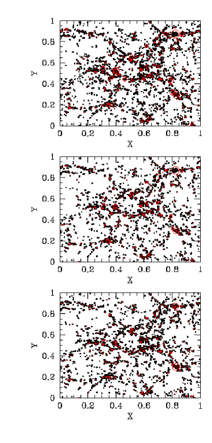
Figure 1: Examples of our galaxy grouping method. Shown is the x-y projection in the L11-Low (top), L11-Medium (middle) and L11-High (bottom) simulations. Black points indicate star particles and red points show galaxies with symbols whose size is proportional to stellar mass.

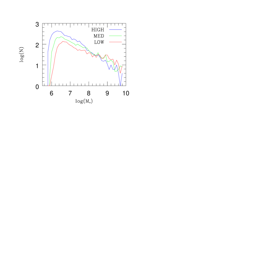
Figure 2: The galaxy mass function for the L11-Low(red), L11-Medium(green) and L11-High(blue) simulations. Note that L11-High has an overabundance of low mass galaxies and a deficit of high mass galaxies relative to L11-Low or L11-Medium indicating that feedback effects are “breaking up” galaxies.

Star particles in the L11 simulations are grouped into galaxies using a friends-of-friends algorithm with a linking length of 0.2 times the mean interparticle spacing. We further require that each galaxy contain at least 20 star particles. Figure 1 shows the positions of star particles and the resulting galaxies projected in the x-y plane for each simulation as an illustrative example. We rank the galaxies in the simulation according to their stellar mass and pick samples above thresholds in stellar mass. There are 1841, 2969, and 5209 galaxies in the L11-Low, L11-Medium and L11-High simulations respectively corresponding to comoving number densities of 1.38, 2.2, and 3.9 $h^{3}{\rm Mpc}^{-3}$. The galaxy (stellar) mass function is shown for each of the simulations in Figure 2. The L11-Low simulation has more high mass objects than either the L11-Medium or L11-High simulations, and conversely, the L11-High simulation has significantly more low mass objects than either the L11-Low or L11-Medium simulations. We expect the supernova energy injection to suppress star formation owing to the heating of the gas, and indeed the total stellar mass in the L11-Low simulation is higher than in the simulations with stronger winds (the stellar mass is dominated by high mass galaxies). It is unclear what process causes an increased abundance of low-mass objects in the L11-High feedback case; the numerical implementation of the supernova energy injection in the simulations probably tends to break up spatial regions of star formation as more energy is injected.

Because of the relatively small box size we use, we do not have many rare objects (i.e., objects of low space density, as LBGs are observed to have). We therefore cannot consider our galaxy samples for these three simulations as LBG samples explicitly, since the estimated number density of LBGs in a box of this size would require us to do our calculations around only a handful of galaxies which would render our statistics quite poor. This partly motivates our decision to analyze additionally the larger-box L25 simulation in which we have sufficient volume to reasonably match the observed space density of LBGs. Star particles in this larger simulation are grouped according to the HOP group algorithm (Eisenstein & Hut, 1998) with threshold parameters $(\delta_{outer},\delta_{saddle},\delta_{peak})=(80,200,240)$ and is described in detail in Nagamine et al. (2001b). We refer the reader to that paper for a more detailed description of the galaxy identification method.

We also use modeled B-band luminosities for the galaxies in the simulation, in order to rank them by luminosity in §4 below. These luminosities are computed by adding the emissivity of all star particles in a galaxy, as determined from the age of the star particle and the instantaneous burst-model isochrone-synthesis code GISSEL99 (see Nagamine et al. 2000 for more details of this procedure).

2.3 Spectral Extraction

For each of the boxes we analyze, we generate a grid of 1200 artificial spectra from the temperature, velocity, and density fields. We extract 400 such sightlines along each projection of the box. Each spectrum has a number of “pixels”, which we set equal to the number of grid cells on a side of the box (432 or 768 pixels for the simulations considered here). We compute Ly$\alpha$ spectra from the temperature, density, and velocity distributions of the gas in the simulation. The spectra are normalized to a fixed mean transmitted flux equal to the observed value of 0.638 at $z=3$ (Press et al., 1993). We use a photoionization rate of $\Gamma_{\gamma,HI}=1\times 10^{-12}s^{-1}$ for the L11 boxes and then multiply the resulting optical depths by small factors in order to ensure that the normalization matches the observed value of the mean flux decrement (0.36). We use the recombination coefficient from Verner & Ferland (1992), and the collisional ionization coefficient from Voronov (1997). Note that collisional ionization may be important for distinguishing the effects of winds close to galaxies where the temperature is high.

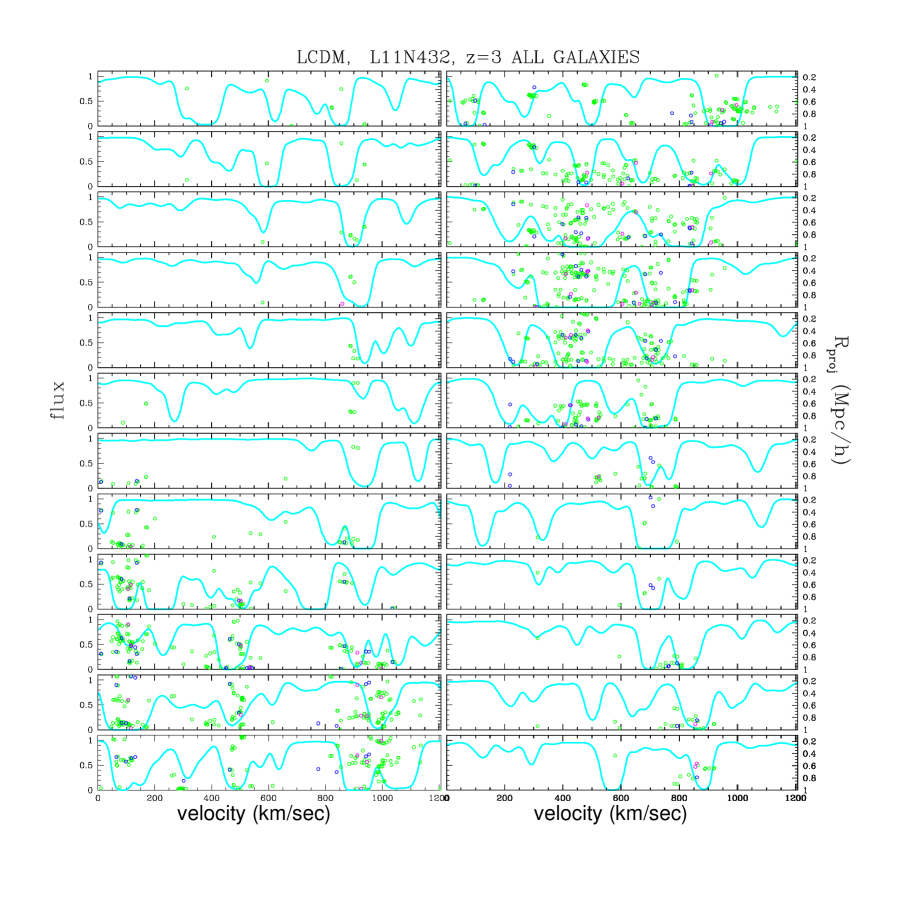
Figure 3: Galaxy-absorption correlations in simulated spectra in the L11-Medium simulation. Symbols show the positions of galaxies located at different redshifts along the sightline located at projected comoving distances as indicated on the right hand axis. Green, blue, magenta symbols correspond to galaxies with masses of $10^{6}<M\leq 10^{8},10^{8}<M\leq 10^{9},>10^{9}M_{\odot}$ respectively. Galaxies lying close to the line of sight are clearly associated with strong absorption features at the galaxy systemic redshift in the simulations.

Examples of simulated spectra from the L11-Medium simulation are shown in Figure 3. The points superposed on the spectra indicate the redshifts and projected distances (right axis of the figure) of galaxies within $1\,h^{-1}\;{\rm Mpc}$ of the sightline. The stellar mass of each galaxy is coded by point color. We see that galaxies lying within $0.5\,h^{-1}\;{\rm Mpc}$ are always associated with strong Ly$\alpha$ absorption. Often, clusters of galaxies are associated with large extended absorption features spanning several hundred $\,{\rm km}\;{\rm s}^{-1}$. Note that strong absorption features are not always associated with galaxies, but galaxies are always close to some absorption feature.

3 Physical Impact of the Winds on the IGM and the Ly$\alpha$ Forest

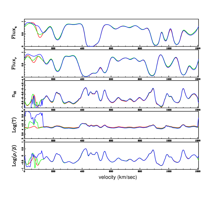
Figure 4: Sample sightline drawn at the same location in each of the L11-Low(red), L11-Medium(green), and L11-High(blue) simulations. Panels (from top to bottom) show the redshift space spectrum, the real space spectrum, the neutral fraction, temperature and density contrast. The redshift-space (observed) flux is not dramatically different between the three simulations despite the fact that temperature and density differences between the sightlines are evident.

To see the typical effect of winds on the Ly$\alpha$  forest spectra, Figure 4 shows spectra from a randomly chosen position in the L11 simulations. The three curves show the same sightline in the L11-Low(red), L11-Medium(green) and L11-High(blue) simulations. The top panel shows the flux as observed in redshift space, and the second panel shows the flux in real space (i.e., with gas peculiar velocities set to zero). The third, fourth and fifth panels show the real-space neutral hydrogen density, temperature, and gas overdensity respectively. The figure shows the well-known correspondence between peaks in the gas density and absorption troughs in the Ly$\alpha$  forest spectrum. Galaxies in the simulations form in the densest central regions of halos, and so they should clearly be associated with deep absorption troughs up to the transverse distance at which galactic halos are surrounded by dense gas.

We also see in Figure 4 that, over most of the spectrum, the three simulations are almost identical, indicating that the effect of winds is very small. The gas temperature is generally highly correlated with gas density. However, we can clearly identify one region of the spectrum in which the three simulations are very different and very high temperatures are reached in regions of widely different densities. This region has obviously been affected by winds. The gas heated by winds can result in weak, broad Ly$\alpha$ features, but this effect is hard to identify and to distinguish from the general Ly$\alpha$ forest arising from colder gas. For example, the Ly$\alpha$ absorption at $v\sim 50\,{\rm km}\;{\rm s}^{-1}$ in this example becomes broader and weaker with increased wind strength, but it seems difficult to statistically detect these changes on the Ly$\alpha$ forest because of the low fraction of the spectrum affected by winds. In fact, as found by McDonald et al. (2004), the effects of galactic winds tend to be degenerate with parameters affecting the typical gas temperature in the IGM, which depends on the uncertain history of heating during helium reionization.

The global behavior of the Ly$\alpha$ forest is more clearly seen in Figure 5, which shows 2-dimensional, 1-cell thick slices through the L11-High, L11-Medium, and L11-Low simulations. We plot the logarithm of the optical depth as a function of spatial position along the vertical axis, and velocity along the horizontal axis. Hence, each horizontal line in the slice shows a spectrum like that in Figure 4 (the transmitted flux shown in Fig. 4 is related to the optical depth as $F=\exp(-\tau)$). Figure 6 shows the same slices (except for a modified color coding for the optical depth), together with the spatial positions (along the vertical axis) and redshifts (along the horizontal axis) of galaxies in the simulation that are located within $1\,h^{-1}\;{\rm Mpc}$ on either side of the sheets. Galaxies with stellar masses larger than $10^{8}M_{\odot}$ are shown in red. The connection between galaxies and the Ly$\alpha$ forest is clearly displayed in Figure 6. Galaxies always lie in regions of high optical depth (because all galaxies within $1\,h^{-1}\;{\rm Mpc}$ of the sheet are shown, a small number of them appear to be displaced from high optical depth regions, but they are all at high optical depths when they are plotted on a slice sufficiently close to the galaxy). There is a remarkable similarity of the optical depth slices among the three simulations, despite the very different wind strengths that were assumed.

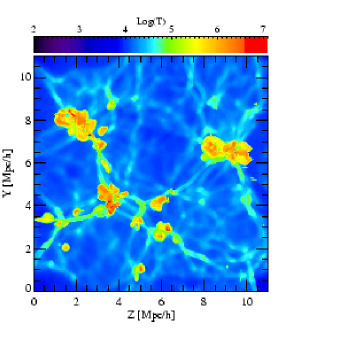
Figure 7: 2-d temperature distribution within the simulations. Slices are now shown in log(T) through the Left: L11-Low, Middle: L11-Medium, and Right: L11-High simulations. The presence of feedback in the temperature structure is clear in these maps. The L11-High simulation shows large bubbles of high temperature gas surrounding “knots” of high density in both the galaxy and optical depth distribution. The temperature bubbles are clearly taking the “path of least resistance” and expanding into the lower density medium perpendicular to the filaments.

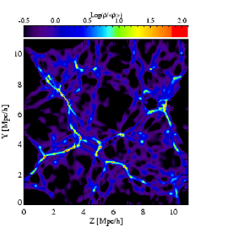
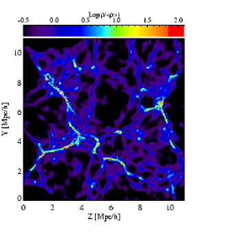
Figure 8: 2-d density distribution within the simulations. Slices are now shown in log($\rho$/${\bar{\rho}}$) through the Left: L11-Low, Middle: L11-Medium, and Right: L11-High simulations. In contrast to the temperature structure, the density structure of the simulation seems remarkably unaltered by the presence of feedback.

To understand this result in terms of the physical properties of the IGM, we plot the temperature and density of the same sheet in real space for the three simulations in Figures 7 and 8. Note that the correspondence to the optical depth sheet shown in Figures 5 and 6 is not exact because the gas peculiar velocities redistribute absorption along the line of sight. The bubbles produced by galactic winds are very clearly seen in the temperature structure. Similar wind structures have been found in other simulations using the SPH technique (e.g., Theuns et al. 2002; Bruscoli et al. 2003). The size of the hot bubbles clearly increases with the strength of the winds. However, the winds do not result in the complete removal of high-density gas near the parent galaxies from which they originate. In fact, Figure 8 shows that the gas density structure is affected only weakly by the winds: comparing the three simulations, we find that the filaments located near the hot bubbles are broken up at a few places on small scales, but apart from this they largely remain in place. The winds have some effect on the optical depth maps of Figures 5 and 6: for example, at the position $Y\simeq 8$ Mpc/h and $Z\simeq 250\,{\rm km}\;{\rm s}^{-1}$, there is a region over which Ly$\alpha$ absorption disappears as the wind strength is increased. This region corresponds to the large hot bubble seen in Figure 7 near this position, and the filament in Figure 8 that is broken in the high-winds simulation at the same position.

Such strong wind effects on the optical depth are, however, relatively rare, and when they occur they tend to redistribute the absorption rather than eliminate it. Most of the time, the hot bubbles expand into low density regions around galaxies, which produce little absorption in any case (see, for example, the region at $Y\simeq 6.5$ Mpc/h, $Z\simeq 8.5$ Mpc/h where a low-density region increases in size with wind strength in Fig. 8). In other words, the winds follow the path of least resistance. Other gas around galaxies may actually get compressed by the wind bubbles and increase its Ly$\alpha$ absorption. Voids in the Ly$\alpha$ spectrum created by the hot expanding bubbles of the winds tend to be filled in by absorption from adjacent gas falling into the galaxy (owing to varying peculiar velocities). The net result is that the effect of winds on the Ly$\alpha$ spectra is rather weak and highly variable among different lines of sight.

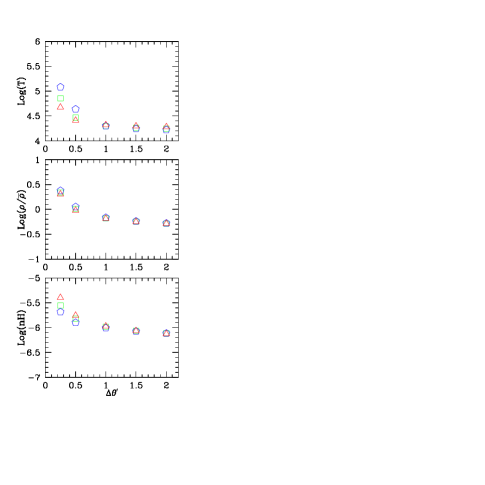
Figure 9: Physical conditions near galaxies within the simulations as a function of wind strength. Median quantities for Top: Log Temperature, Middle: Log gas overdensity, Bottom: Log neutral density for the Low (red triangles), Med (green squares), and High (blue pentagons) simulations. The temperature is clearly higher in the High feedback simulation than in the Medium or Low simulations but the density is only slightly lower. The neutral density continues to rise close to galaxies in all simulations, although the absolute value is lower in the High feedback simulation due to the increased temperature.

Figure 9 quantifies the impact of winds on the physical state of the gas in the neighborhood of galaxies. We show the median value of the temperature, gas overdensity, and neutral hydrogen density in all the simulation pixels whose distance to any identified galaxy is within the value on the horizontal axis. The temperature increase and neutral density decrease with wind strength is apparent here. Note, however, that even in the simulation with the strongest winds the neutral density continues to rise as a galaxy is approached. Curiously, the total gas density is not much affected by the winds; if anything it tends to increase slightly with wind strength. These effects of winds on the physical state of the gas are the direct cause of any changes in the Ly$\alpha$ forest transmission close to galaxies.

4 Flux Statistics

Here we quantify the relation between the Ly$\alpha$ forest flux statistics and the proximity to galaxies in the simulation, and the way this relation varies with wind strength.

4.1 The Conditional Flux Decrement PDF

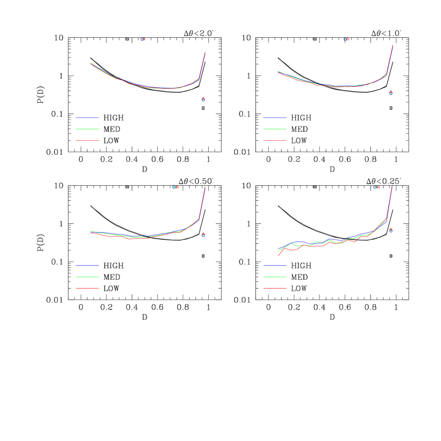
Figure 10: Conditional flux decrement PDF as a function of wind strength. PDFs are computed for all galaxies within the L11-Low(red), L11-Medium(green) and L11-High(blue) simulations. Black curves show the unconditional PDF for each simulation. Panels indicate decreasing separation between galaxies and the sightline in arcminutes as indicated in top right hand corner of each panel. Symbols along the top of each panel show the mean of the distributions and symbols along the right hand side indicate the fraction of pixels in each distribution with flux decrement $0.9\leq{\rm D}\leq 1.0$ for each simulation. Red triangles, green squares and blue pentagons correspond to the L11-Low,Medium and High simulations respectively. The conditional flux PDFs are remarkably insensitive to galactic winds.

In general, one can codify the influence of a galaxy on the Ly$\alpha$ forest by the probability distribution function (PDF) of the flux decrement, $D$ (equal to one minus the fraction of transmitted flux), conditioned on the presence of a galaxy within a transverse angular separation $\Delta\theta$ and velocity separation $\Delta v$. We first study this conditional flux PDF (CPDF) for $\Delta v=0$, which was studied previously by Kollmeier et al. (2003a) using SPH simulations and is described in more detail there. We obtain the CPDF using all resolved galaxies (defined as having at least 20 star particle members) in each simulation. For each galaxy, random lines of sight that pass within a maximum impact parameter $\Delta\theta$ are chosen, and the flux decrement at the pixel that has the same redshift as the galaxy (taking into account the galaxy peculiar velocity) is selected. Note that by choosing lines of sight uniformly distributed within a maximum impact parameter, we are averaging the CPDF over impact parameters with a weighting proportional to $\Delta\theta\,d\Delta\theta$, up to the maximum impact parameter shown in each panel. The CPDF of the flux decrement is shown in Figure 10 for the four values of $\Delta\theta$ (in arcminutes) indicated in the top right corner of each panel. The results are shown for the three L11 simulations with different wind strengths. The black solid lines show the unconditional PDF computed using all pixels in all spectra.

As the transverse galaxy-sightline distance is reduced, there is a shift in the CPDF from unsaturated (low D) pixels to saturated (high D) pixels. The values of the mean decrement (shown as the top symbols) and the probability of saturated pixels, defined as $D>0.9$ (right symbols), which capture some of the information of the full CPDF, also show this clearly. This result simply reflects the association of galaxies with regions of high optical depth shown earlier in Figure 6 and is in good agreement with the results of Kollmeier et al. (2003b).

The wind effects are seen to be small, as expected from the optical depth sheets discussed in the previous section. These weak wind effects on the Ly$\alpha$ forest are in agreement with the work of Theuns et al. (2002) and Bruscoli et al. (2003) using a different simulation method with different wind prescriptions. The result also agrees with that of Croft et al. (2002); Kollmeier et al. (2003b); Weinberg et al. (2003) and Desjacques et al. (2004), who examined simple “bubble” wind models. The small difference has the expected sign: stronger winds should and do reduce the Ly$\alpha$ absorption in the regions from which they emerge.

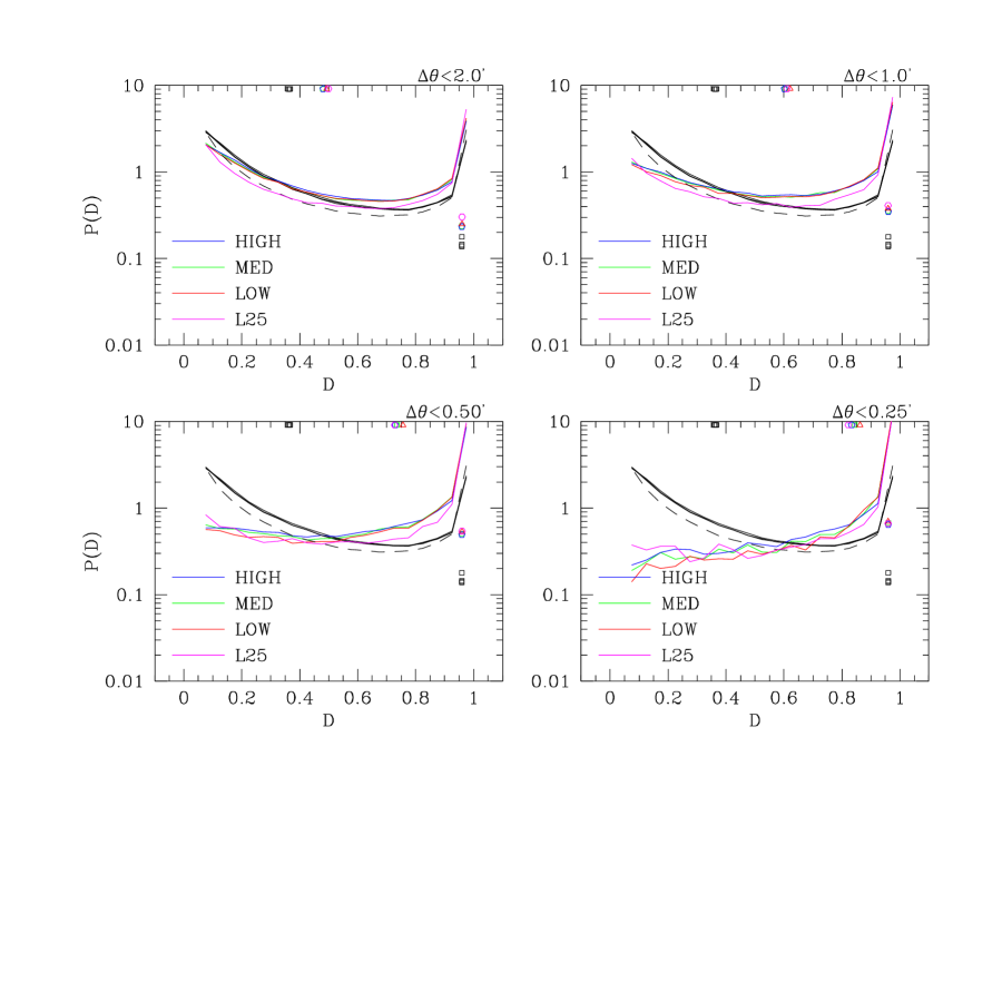
Figure 11: Effect of box size on conditional flux decrement PDF. PDFs are computed for all galaxies within the L11-Low(red), L11-Medium(green), L11-High(blue) and L25 (magenta) simulations. Panels indicate decreasing separation between galaxies and the sightline in arcminutes as indicated in top right hand corner of each panel. The unconditional flux decrement is shown for the L11 simulations (black solid lines) and the L25 simulation (black dashed lines). Symbols along the top of each panel show the mean of the distributions and symbols along the right hand side indicated the fraction of pixels in each distribution with flux decrement $0.9\leq{\rm D}\leq 1.0$ for each simulation. Red triangles, green squares and blue pentagons correspond to the L11-Low,Medium and High simulations respectively. Magenta hexagons correspond to the L25 simulation. The L25 simulation has different unconditional flux PDF due to the larger scale modes that are allowed in this box. The conditional flux PDFs, however, are at the expected level of agreement given the differences in box size and parameters between the four simulations.

In Figure 11, we compare the PDFs for all four of our simulations. The small difference in the unconditional flux PDFs between the L25 simulation (dashed black line) and the three L11 simulations (solid black lines) is due to a combination of the effect of differing box size and the slightly different power spectra adopted in the large and small boxes. Simulations of small boxes have an artificially low dispersion in the flux decrement that arises from a low dispersion in gas density distribution, owing to the suppression of large-scale fluctuations.

In summary, the unconditional and conditional PDF of the flux decrement are robust predictions of the CDM model, and the effects of galactic winds on them are small.

4.2 Dependence of the Conditional PDF on Galaxy Luminosity

The conditional PDF can also be examined as a function of galaxy luminosity to see whether more luminous galaxies tend to be associated with stronger Ly$\alpha$ absorption. In Kollmeier et al. (2003b), variations of Ly$\alpha$ absorption around galaxies were shown to have little dependence on the total star formation rate in each galaxy. The Eulerian simulations we use here have a different prescription for estimating galaxy luminosity (see §2), and they incorporate the effects of winds, which can affect galaxies of different luminosities in different ways.

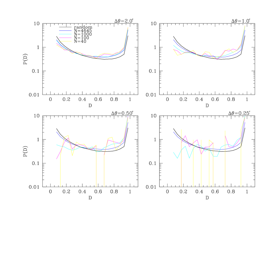
Figure 12: Effect of galaxy luminosity on conditional flux decrement PDFs. Curves show different galaxy samples selected by increasing thresholds in B-band luminosities. The calculation computed around all galaxies is shown in blue, the 1000 brightest galaxies (cyan), the 100 brightest galaxies (magenta), and the 40 brightest galaxies (yellow). Panels show decreasing maximum angular separation $\Delta\theta^{\prime}$ (indicated in the upper right hand corner of each panel). The yellow curve in each panel shows the brightest galaxies whose number density matches that of observed LBGs (Adelberger et al., 1998, 2004). The expected trend of increased saturated fraction with decreasing sightline-galaxy separation is clear. However, there is no strong dependence of the PDF on luminosity. The paucity of galaxy-sightline pairs make the closest-separation, smallest-number curves noisy.

We explore the dependence on galaxy luminosity in Figure 12, which shows the CPDF in the L25 simulation within four different impact parameters and for galaxies with luminosity above four different thresholds. The four luminosity thresholds (with luminosities computed as described in §2.2) are $7.124\times 10^{9}$, $3.358\times 10^{9}$, $2.809\times 10^{8}$, and $9.102\times 10^{5}L_{\odot}$, and the total number of galaxies in the $25\,h^{-1}\;{\rm Mpc}$ box of the simulation above each luminosity threshold is labeled for each curve. For reference, the space density of the observed LBGs would correspond to our highest luminosity threshold, with only $N=40$ galaxies in the simulation. The figure shows there is a weak dependence of the galaxy-Ly$\alpha$ transmission correlation on galaxy luminosity. The sign of the effect is as expected if galaxy luminosity correlates with mass and large-scale environment—the Ly$\alpha$ forest around more luminous galaxies shows a preference for high decrement pixels. This dependence on galaxy luminosity is, of course, sensitive to the relation between observed galaxies and galaxies in the simulation, which is affected by our poor understanding of the factors that determine star formation rates in galaxies. At the smallest angular separations, the dependence of the galaxy-Ly$\alpha$ transmission correlation cannot be clearly distinguished from the random noise on the curves caused by the small number of galaxy-sightline pairs at these separations in our box. It is clear, however, that in all cases the Ly$\alpha$ absorption increases as a galaxy is approached.

4.3 Dependence on Velocity Offset

The preceding figures show only the CPDF of the flux decrement at the same velocity as a galaxy within a certain impact parameter. However, we expect the galaxy-intergalactic medium connection to persist over some velocity range from the true redshift of the galaxy. One can choose to examine pixels within a fixed velocity interval from the galaxy redshift as a further test of the predictions. We now examine the flux distribution as a function of velocity offset.

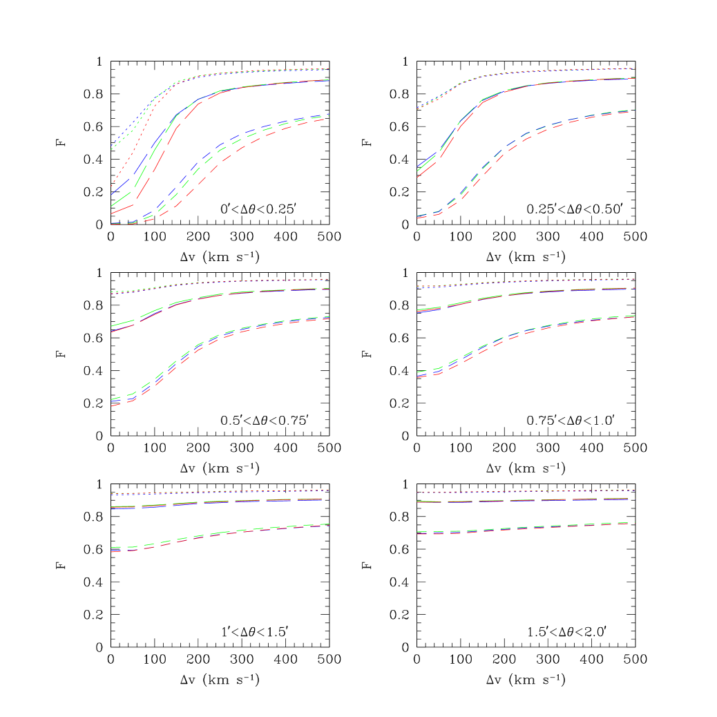
Figure 13: Flux distribution as a function of galactic wind strength. The $10\%$ (dotted),$25\%$ (long dashed), and $50\%$ (short dashed) values of the flux as a function of galaxy proximity in pixels in annuli of $\Delta\theta$ and averaged over a velocity interval $\pm\Delta v$ of the 100 most massive galaxies in the L11-Low (red), L11-Med (green), and L11-High (blue) simulations corresponding to $\epsilon_{SN}=3\times 10^{-7},3\times 10^{-6}$ and $1.5\times 10^{-5}$ respectively. The likelihood of observing high transmitted flux close to galaxies is greater in the High simulation indicating that feedback has an effect on some pixels.

In Figure 13 we show the median, first quartile and 10 percentile values of the transmitted flux, F, for Ly$\alpha$ forest spectral pixels in lines of sight within annuli of angular separation from a galaxy in the range $\theta_{1}<\Delta\theta<\theta_{2}$, and within a velocity interval $\pm\Delta v$. The 100 most massive galaxies in the simulation have been used for this calculation. Hence, the (top, middle, bottom) curve in each panel gives the value of the transmitted flux for which the probability to measure a larger flux is $0.1$, $0.25$, and $0.5$, respectively, over the indicated range of $\Delta\theta$ and at any pixel in the spectrum within $\pm\Delta v$. The six panels are for six different ranges of $\Delta\theta$, as shown. The red, green and blue curves correspond to the L11-Low, L11-Medium and L11-High simulations, respectively. In the limit of large $\Delta v$, the curves generally approach the unconditional percentile values. The decrease of $F$ at small $\Delta v$ shows that it becomes increasingly unlikely to observe large transmitted fluxes as one probes pixels closer to the galaxy redshift.

We note from Figure 13 that the effects of winds are most important within an impact parameter $\Delta\theta<0.25^{\prime}$ and that they are small at larger separations. We also point out that the probability of observing a transmitted flux value as high as $\sim 0.8$ near a galaxy decreases rapidly only at $\Delta v\lesssim 150\,{\rm km}\;{\rm s}^{-1}$, and that at larger velocity separations this probability is not much affected by the presence of winds (see top left panel). In other words, close to the galaxy’s systemic velocity, the probability of finding a transparent line of sight is low but is significantly increased by winds, while at large offsets from the galaxy redshift the probability is higher but is no longer sensitive to winds. The median transmitted flux, typically with a lower value $\sim 0.1$ to $0.6$, is more strongly affected by winds up to velocity separations $\Delta v\sim 300\,{\rm km}\;{\rm s}^{-1}$. As seen in Figure 13, the effects of winds should be detectable in the Ly$\alpha$ forest near galaxies once the median transmitted flux is measured to an accuracy better than $\sim 10\%$.

The results obtained from the L11 simulations are, however, strongly affected by the size of the simulation box, and better theoretical predictions from larger boxes will be needed in order to infer wind strengths from the transmitted flux distribution as a function of $\Delta v$ and $\Delta\theta$. The total velocity across the box in the L11 simulations is only $\sim 1200\,{\rm km}\;{\rm s}^{-1}$, so the velocity interval $\Delta v=300\,{\rm km}\;{\rm s}^{-1}$ shown in Figure 13 is nearly half of the box size. The curves in this figure are strongly affected by the box size: they increase too fast with $\Delta v$ due to the suppression of large-scale power. Any box-size effects should be smaller in the L25 simulation. The same curves for this simulation, computed for the set of the 100 most luminous galaxies, are shown in Figure 14. These curves are more reliable predictions for a direct comparison to observations than those in Figure 13. Unfortunately, we do not have simulations for different wind strengths in larger boxes. However we expect that the differences introduced by winds would be similar to those in the L11 simulations.

5 Comparison with Observations

The correlation of LBGs and the Ly$\alpha$ forest has been studied observationally by Adelberger et al. (2003), who measured the mean flux decrement ($\langle D\rangle=\langle 1-F\rangle$, where $F$ is the transmitted flux, which was shown in Figs. 13 and 14) as a function of total redshift-space comoving separation from a galaxy, $\Delta$. This is defined in terms of the angular and velocity separations as

$$\Delta^{2}=\left[D_{a}(z)(1+z)\Delta\theta\right]^{2}+\left[(1+z)\Delta v/H(z)\right]^{2}~{},$$ (4)

where $D_{a}(z)$ and $H(z)$ are the angular diameter distance and the Hubble parameter at redshift $z$. The Adelberger et al. (2003) observations are reproduced in Figure 15, together with our predictions for the same quantity using the L25 simulation. We use four different galaxy luminosity thresholds, such that the total number of galaxies in the simulation above the threshold is 1000, 100, 40 and 20.

As previously found by several authors, the results of Adelberger et al. (2003) do not agree with theoretical expectations. The observations show the flux decrement at a constant value for $\Delta<3\,h^{-1}\;{\rm Mpc}$, which then drops sharply at $\Delta<0.5\,h^{-1}\;{\rm Mpc}$. The predictions show that the flux decrement should continually increase as a galaxy is approached. The effects of winds in our simulations do not alter the clear increase of the flux decrement, relative to its mean value, as $\Delta$ decreases from $3\,h^{-1}\;{\rm Mpc}$ to $0.5\,h^{-1}\;{\rm Mpc}$, and they may produce at most a $\sim 10\%$ decline of the flux decrement when $\Delta<0.5\,h^{-1}\;{\rm Mpc}$ for the most luminous galaxies. However, this small decline, seen in the innermost point in Figure 15 for the most luminous galaxy class, may be affected by noise due to the small number of galaxy-quasar pairs at this small separation in the simulation. The observational points at small $\Delta$ in Figure 15 challenge the CDM-based picture of the Lyman-alpha forest that has emerged over the last decade. This picture predicts that the average flux decrement near galaxies should increase, not decrease. The galactic winds predicted by our simulations reduce the strength of this trend but do not reverse it, in agreement with other studies (Croft et al., 2002; Kollmeier et al., 2003a, b; Bruscoli et al., 2003; Desjacques et al., 2004).

We now ask whether the discrepancy seen in Figure 15 could be explained by galaxy redshift errors, misestimation of the continuum, or simply by small number statistics. We focus on the innermost point, based on three quasar-galaxy pairs with separations of $16^{\prime\prime}$, $17^{\prime\prime}$, and $21^{\prime\prime}$, for which Adelberger et al. (2003) find a mean flux decrement of 0.11. We calculate the probability of obtaining this measured value, given the model of the L25 simulation we have analyzed in previous sections.

Redshifts of faint LBGs are notoriously difficult to obtain because the gas being expelled in a wind at small radius can displace the redshift of emission or absorption lines relative to the systemic galaxy redshift. After correcting for this effect, Adelberger et al. (2003) estimated their galaxy redshift errors were $\sigma_{v}\simeq$ $150\,{\rm km}\;{\rm s}^{-1}$ (according to a calibration of the redshift error that Adelberger et al. (2003) measured from an independent sample of 27 Lyman break galaxies with well measured nebular emission line redshifts), but could be larger for some galaxies when line equivalent widths are not measured, or in some pathological cases where galaxy wind effects are apparently stronger. Previous analyses (Croft et al., 2002; Kollmeier et al., 2003a) found that errors in the galaxy redshifts drawn from a Gaussian with dispersion $300\,{\rm km}\;{\rm s}^{-1}$ substantially reduce the predicted transmitted flux close to galaxies, but are insufficient to explain the very low mean flux decrement ($\langle D\rangle\sim 0.1$) that Adelberger et al. (2003) measured at the smallest value of $\Delta$ (see Fig. 15). To estimate this effect within the context of the present simulations, we calculate the cumulative distribution of predicted decrements, $D$, averaged over velocity widths $\pm\Delta v$, assuming various different velocity errors, $\sigma_{v}$. That is, in our simulation, we make our average decrement measurement over a velocity range $\pm\Delta v$, centered at a redshift displaced from the true redshift of the galaxy by a random amount drawn from a Gaussian of dispersion $\sigma_{v}$. Here we use the L25 simulation because of its larger volume. Figure 16 shows our results for several choices of the averaging interval $\Delta v$. Adelberger et al. (2003) binned their data by $\Delta v\sim(41,39,24)\,\rm km\,s^{-1}$, for the quasars SSA22D13, Q1422+2309b and Q0201+1120 respectively. These values are bracketed by the top and second rows of panels. Right hand panels show the cumulative probability distributions for a single galaxy-quasar pair, while left hand panels show the distributions for the mean decrement averaged over three galaxy-quasar pairs selected at random from our full sample.

Note that while we average over velocity bins of fixed width, Adelberger et al. (2003) average over a variable width that depends on impact parameter. However, since the range of their velocity width is small and bracketed by the upper and middle panels in our Figure 16 that are essentially identical, this difference has no practical impact.

While redshift errors substantially increase the probability of low decrements, even for $\sigma_{v}=300\,{\rm km}\;{\rm s}^{-1}$ the probability of a single galaxy-quasar pair having decrement $D<0.11$ is only $\sim 15\%$ for an averaging interval $\Delta v=50\,{\rm km}\;{\rm s}^{-1}$ (middle right panel), and the probability of the mean decrement of three such pairs being below 0.11 is $\sim 1\%$. We note that for at least one of the three galaxies, the redshift error has been confirmed to be less than $60\,{\rm km}\;{\rm s}^{-1}$ (K. Adelberger, private communication). These probabilities are higher than obtained in windless simulations (Kollmeier et al., 2003a), indicating that winds affect the flux distribution, but not enough to make the observations likely.

In addition to an observational redshift error, there may also be an intrinsic redshift error arising from the fact that real galaxies may have an intrinsic velocity dispersion relative to the surrounding gas at the observed impact parameters that is not fully included in our simulations. The resulting intrinsic redshift error needs to be added in quadrature to the observational one. In galaxy groups, the group velocity dispersion has the same effect as a redshift error. The simulations we use have limited spatial resolution, implying that the high-density central parts of halos are not well resolved, and the orbits of satellite galaxies and their tidal disruption are not adequately followed. This results in an artificial increase of the merger rate of galaxies in groups, which can reduce the velocity dispersion of simulated galaxies compared to real galaxies. The magnitude of this theoretical redshift error actually depends on the nature of the Lyman break galaxies. If these are often satellite galaxies undergoing intense starbursts after a group merger (e.g., Somerville et al. 2001), they may be moving close to the escape velocity of the galaxy group halo and have large peculiar velocities relative to the surrounding gas. If they are more often associated with central halo galaxies, the peculiar velocities may be lower. For a singular isothermal halo with velocity dispersion $\sigma$ and outer radius $r_{h}$, the escape velocity at radius $r$ is

$$v_{esc}=2\sigma\sqrt{1+\log(r/r_{h})}~{}.$$ (5)

For a typical galaxy group halo at $z\sim 3$ with $\sigma\sim 200\,{\rm km}\;{\rm s}^{-1}$, the escape velocity may easily be as large as $600\,{\rm km}\;{\rm s}^{-1}$, which after projection may give a velocity dispersion comparable in magnitude to the observational errors. In other words, the total redshift error may be substantially increased relative to the observational redshift error. Even f we assume, however, total redshift errors of $600\,{\rm km}\;{\rm s}^{-1}$ (which we view as unrealistically large), the joint probability for three quasar-galaxy sightlines is only $\sim 4\%$. Alternatively, the high stellar masses estimated for LBGs (Shapley et al., 2001) suggest that they are most likely the central galaxies of their parent halos, in which case their peculiar velocities relative to the halo center-of-mass are likely to be small and the intrinsic redshift errors, also small. Observations of the clustering of LBGs in redshift space and the pairwise velocity dispersion of LBGs as a function of angular separation should reflect the intrinsic dispersion of galaxy redshifts from the redshift of the surrounding gaseous halos distinguishing between the two possible scenarios (central vs. satellite galaxies) and constraining our estimates of the size of this effect.

Continuum fitting errors could affect the observational estimates of the mean decrement. At the redshift of the Adelberger et al. (2003) observations, the minimum flux decrement over intervals of $\sim 3000\,{\rm km}\;{\rm s}^{-1}$, comparable to the intervals used for continuum fitting, is usually no more than $\sim 2\%$, so it is unlikely that the continuum fitting error is larger than that. Spectral noise can also affect the probability of measuring the low flux decrement of Adelberger et al. (2003). The noise in their spectrum over an interval $\Delta v=20\,{\rm km}\;{\rm s}^{-1}$ is only $\sim 0.02$. The true flux decrement in the first data point of Figure 15 may be as high as $0.15$, owing to the combination of continuum fitting errors and spectral noise. The probability to measure this value of the flux decrement for three galaxies, and for a total redshift error of $\sigma_{v}=300\,{\rm km}\;{\rm s}^{-1}$ would still be $\sim 2\%$, from our Figure 16.

An alternative test that can be done to compare the model predictions with present and future data is to average the flux decrement over a larger interval $\Delta v$. This has the advantage of reducing the sample variance of the measured flux decrement, and the disadvantage of eliminating information from flux fluctuations on scales smaller than $\Delta v$. In particular, if the galaxy redshift error is $\sigma_{v}=300\,{\rm km}\;{\rm s}^{-1}$, then it makes sense to consider the average flux over $\Delta v=300\,{\rm km}\;{\rm s}^{-1}$ interval because the spectral points over this interval are similarly likely to be at the true galaxy redshift. We have estimated by eye from Figure 10 of Adelberger et al. (2003) that the flux decrement of the same three galaxies when averaged over $\Delta v=300\,{\rm km}\;{\rm s}^{-1}$ around the galaxy redshift is $0.29$. Figure 16 shows that the probability of this flux is only $\sim 2\%$ indicating that this larger-scale feature is also not easily explained by our simulated spectra.

In agreement with Kollmeier et al. (2003a), we find that the small number of galaxies in the observed sample do not easily explain the discrepancy between the simulation predictions and the Adelberger et al. (2003) data, even if we consider the dominant contributions of galactic winds and redshift errors. Fortunately, the size of these kinds of data sets is bound to increase over the next few years, and comparison of larger data sets to predictions of the type presented here should definitively show whether there is or is not a contradiction between the models and the observations.

6 Discussion and Conclusions

We have analyzed the Ly$\alpha$ forest in the neighborhood of galaxies using cosmological simulations of structure formation that include galactic winds. We find that winds can greatly affect the temperature structure of intergalactic gas that is relatively close to galaxies, but that the density structure is less affected. Changes in the structure of the optical depth giving rise to the Ly$\alpha$ forest are smaller still than in the density field because of the tendency of peculiar velocities to smear out the changes in regions affected by winds. These results are broadly in accordance with previous studies that used SPH simulations with a variety of prescriptions for modeling the effects of galactic winds (Theuns et al., 2002; Bruscoli et al., 2003), as well as with more simplified models (Croft et al., 2002; Kollmeier et al., 2003a, b; Desjacques et al., 2004).

Analysis of simulations with realistic wind prescriptions is particularly interesting in light of recent observations of the galaxy-Ly$\alpha$ forest connection at $z=3$ (Adelberger et al., 2003) and the apparent detection of a “galaxy proximity effect”. While more data are clearly needed in order to ensure that the result is not due to the small number of galaxy-QSO pairs observed so far, we find that our simulations are not successful in reproducing the magnitude of the proximity effect observed, except as a rare statistical fluctuation. Intrinsic galaxy velocity dispersions, caused by the motion of the galaxies within the gaseous halos around them, may increase the effective galaxy redshift error. This effect is highly uncertain from a theoretical perspective, because it depends on the type of halos in which LBGs form (in particular, whether LBGs tend to be massive galaxies in halo centers, or faster-moving satellite galaxies), but may make the current observations more likely.

The Ly$\alpha$ flux decrement is generally predicted to increase near galaxies owing to the high gas density in regions that have gravitationally collapsed. Winds have the effect of diminishing the magnitude of this increase. This effect of winds, although small, is in principle detectable, in particular by complementing Ly$\alpha$ measurements with metal-line observations that could be sensitive to the gas temperature, although we have not investigated the effect on metal-lines in this paper. To detect the effect of winds in reducing the Ly$\alpha$ absorption near galaxies, accurate theoretical predictions are required for the expected Ly$\alpha$ flux decrement distribution as a function of velocity and angular separation from a galaxy, for different wind strengths. We have presented these predictions here, although with the caveat that the predictions may depend on the uncertain correspondence of observed Lyman break galaxies and the galaxies in the simulations we analyze. A large number of galaxies with high signal-to-noise quasar spectra (similar to those used in the Adelberger et al. 2003 study) from nearby sightlines are essential to search for the effects of winds. As shown in our Figures 13 and 14, large redshift errors and averaging the flux over large intervals in velocity will seriously affect the measurement of the effect of winds on the galaxy-Ly$\alpha$ absorption correlation, since the signature of winds is strongest close to the galaxies’ systemic velocities. Accurate determination of the clustering properties of LBGs (or other high-redshift galaxy samples in which the selection function is well understood) in redshift space should allow us to correct for the effect of intrinsic galaxy redshift errors on the observed galaxy-Ly$\alpha$ correlation for future comparisons. With precise redshifts and high-resolution spectra, the effect of winds at small separations is detectable.

Ongoing observations will provide a large increase in the sample of galaxies used to determine the mean Ly$\alpha$ transmitted flux near LBGs (Adelberger et al. , 2005). These observations will result in a dramatic improvement in our assessment of the effects of winds on the Ly$\alpha$ forest observed near galaxies.

Table 1: Simulation Parameters

Name	$L_{\rm box}$ $(\,h^{-1}\;{\rm Mpc})$	$N_{cell}$	$\epsilon_{\rm SN}$	$\Omega_{m}$	$\Omega_{\Lambda}$	$\Omega_{b}$	$h$	$\sigma_{8}$	$n$
L11-High	$11$	$432^{3}$	$1.5\times 10^{-5}$	$0.29$	$0.71$	$0.047$	0$.70$	$0.85$	$1.0$
L11-Medium	$11$	$432^{3}$	$3\times 10^{-6}$	$0.29$	$0.71$	$0.047$	0$.70$	$0.85$	$1.0$
L11-Low	$11$	$432^{3}$	$3\times 10^{-7}$	$0.29$	$0.71$	$0.047$	0$.70$	$0.85$	$1.0$
L25	$25$	$768^{3}$	$1\times 10^{-5}$	$0.30$	$0.70$	$0.035$	0$.67$	$0.9$	$1.0$

Figure 5: 2-d Optical depth distributions within the simulations. Slices are 1 simulation cell thick, cut midway through the Left: L11-Low, Middle: L11-Medium, and Right: L11-High simulations. Color codes are as indicated on top of each panel. These optical depth maps show clearly the filament-void structure that is a universal feature of the concordance cosmological model. The horizontal features are due to redshift-space distortions (the “finger-of-god” effect).

Figure 6: Relation between galaxies and optical depth within the simulations. Slices are 1 simulation cell thick, cut midway through the Left: L11-Low, Middle: L11-Medium, and Right: L11-High simulations. Color codes are as indicated on top of each panel. All galaxies within $1\,h^{-1}\;{\rm Mpc}$ on either side of the slice are shown at their locations by black symbols. In general, galaxies trace the filaments in the dark matter, and hence the gas and optical depth, distributions. The positions of galaxies with stellar masses larger than $10^{8}M_{\odot}$ are indicated by the red symbols.

Figure 14: Flux distribution for the L25 simulation (magenta curves). The $10\%$ (dotted), median (short dashed), and $25\%$ (long dashed) values of the flux as a function of galaxy proximity in pixels in annuli of $\Delta\theta$ and averaged over $\pm\Delta v$ of the 100 most luminous galaxies in the simulation. The box size and galaxy number density affect these curves strongly.

Figure 15: Comparison of predictions from L25 with recent observations by Adelberger et al. 2003. Shown are the results for the mean flux decrement $\langle D\rangle$ as a function of redshift-space separation, $\Delta$ and space density for $N=20$(red triangles),$N=40$ (green squares), $N=100$ (blue pentagons) and $N=1000$ (magenta hexagons) simulations compared with the Adelberger et al. 2003 observations (filled points). The detailed shapes of these curves seems dependent on galaxy number density, although this may be due to the poorer statistics with the smaller galaxy samples.

Figure 16: Cumulative distribution of the average flux decrement near LBGs as functions of redshift error and spectral resolution. Right hand panels show the decrement, D, for individual galaxies within the simulation and left hand panels show the average decrement, $\langle D\rangle$ for galaxy triplets. Upper, middle, and lower panels show the averages for velocity intervals $\Delta v=\pm 20,50,100,300\,{\rm km}\;{\rm s}^{-1}$ respectively. Curves show the cumulative distribution as a function of galaxy redshift errors. Errors in the galaxy redshifts are drawn from a Gaussian distribution of zero mean and dispersion, $\sigma$. Red, green, blue and cyan curves show the cases for $\sigma_{v}=0,150,300,$ and $600\,{\rm km}\;{\rm s}^{-1}$ respectively. The galaxy sample is chosen according to a luminosity threshold such that the observed number density of LBGs is matched. The angular separation between the galaxies and sightlines is chosen to correspond to the three closest galaxy-QSO separations in Adelberger et al. (2003).

References

- Adelberger et al. (1998) Adelberger, K. L., Steidel, C. C., Giavalisco, M., Dickinson, M., Pettini, M., & Kellogg, M. 1998, ApJ, 505, 18
- Adelberger et al. (2003) Adelberger, K.L., Steidel, C.C., Shapley, A.E., Pettini, M. 2003, ApJ, 584,45 (ASSP)
- Adelberger et al. (2004) Adelberger,K.L., Steidel, C.C., Pettini, M., Shapley, A.E., Reddy, N.A., Erb, D.K., 2004, ApJin press
- Aguirre et al. (2001) Aguirre, A., Hernquist, L., Weinberg, D., Katz, N., & Gardner, J. 2001, ApJ, 560, 599
- Bruzual & Charlot (1993) Bruzual, A. G. & Charlot, S. 1993, ApJ, 405, 538
- Bruzual (2000) Bruzual, A. G. 2000, preprint (astro-ph/0011094)
- Bruscoli et al. (2003) Bruscoli, M., Ferrara, A., Marri, S., Schneider, R., Maselli, A., Rollinde, E., Aracil, B., MNRAS, 343, L41
- Cen & McDonald (2002) Cen, R., & McDonald, P. 2002, ApJ, 570, 457
- Cen & Ostriker (1992) Cen, R., & Ostriker, J. P. 1992, ApJ, 393, 22
- Cen & Ostriker (1999) Cen, R., & Ostriker, J. P. 1999, ApJ, 514, 1
- Cen & Ostriker (2000) Cen, R., & Ostriker, J. P. 2000, ApJ, 538, 83
- Cen et al. (2004) Cen, R., Nagamine, K., & Ostriker, J.P., 2004, submitted to ApJ (astro-ph/0407143)
- Croft et al. (2002) Croft, R.A.C., Hernquist, L., Springel, V., Westover, M., & White, M. 2002, ApJ, 580, 634
- Deharveng et al. (2001) Deharveng, J.-M., Buat, V., Le Brun, B., Milliard, B., Kynth, D., Shull, J. M., & Gry, C. 2001, A&A, 375, 805
- Dekel & Silk (1986) Dekel, A., & Silk, J. 1986, ApJ, 303, 39
- Desjacques et al. (2004) Desjacques, V., Nusser, A., Haehnelt, M.G., Stoehr, F., MNRAS, 351, 1395
- Edelson & Malkan (1986) Edelson, R.A., & Malkan, M.A., 1986, ApJ, 308, 59
- Eisenstein & Hut (1998) Eisenstein, D., & Hut, P., 1998 ApJ, 498, 137
- Ferland et al. (1992) Ferland, G. J., Peterson, B. M., Horne, K., Welsh, W. F., & Nahar, S. N. 1992, ApJ, 387, 95
- Fukugita et al. (1998) Fukugita, M, Hogan, C.J., & Peebles, P.J.E. 1998, ApJ, 503, 518
- Heckman et al. (1998) Heckman, T., et al. 1998
- Heckman et al. (2001) Heckman, T. M., Sembach, K. R., Meurer, G. R., Leitherer, C., Calzetti, D., & Martin, C. L. 2001, ApJ, 558, 56
- Hurwitz et al. (1997) Hurwitz, M., Jelinsky, P., & Dixon, W. V. D. 1997, ApJ, 481, L31
- Kollmeier et al. (2003a) Kollmeier, J.A., Weinberg, D.H., Davé, R., & Katz, N. 2003, ApJ, 594, 75
- Kollmeier et al. (2003b) Kollmeier, J.A., Weinberg, D.H., Davé, R., & Katz, N. 2003, in The Emergence of Cosmic Structure eds. S. Holt & C. Reynolds, AIP Conference Proceedings, New York, p.191, (astro-ph/0212355)
- Martin (1998) Martin, C., L., 1998,ApJ, 506, 222
- McDonald et al. (2002) McDonald, P., Miralda-Escudé, J., & Cen, R. 2002, ApJ, 580,42
- McDonald et al. (2004) McDonald, P., Seljak, U., Cen, R., Bode, P., & Ostriker, J. P. 2004, sumbitted to MNRAS(astro-ph/0407378)
- Nagamine et al. (2000) Nagamine, K., Cen, R., & Ostriker, J.P., 2000, ApJ, 541, 25
- Nagamine et al. (2001a) Nagamine, K., Fukugita, M., Cen, R., & Ostriker, J.P., 2001a, MNRAS, 327,L10
- Nagamine et al. (2001b) Nagamine, K., Fukugita, M., Cen, R., & Ostriker, J.P., 2001b, ApJ, 558, 497
- Ostriker & Cowie (1981) Ostriker, J.P., & Cowie, L., 1981, ApJ, 243, 127
- Pettini et al. (2002) Pettini, M., Rix, S. A., Steidel, C. C.,Adelberger, K. L., Hunt, M. P., & Shapley, A. E. 2002, ApJ, 569, 742
- Press et al. (1993) Press, W. H., Rybicki, G. B., & Schneider, D. P. 1993, ApJ, 414, 64
- Sazonov et al. (2004) Sazonov, S. Y., Ostriker, J. P., & Sunyaev, R. A. 2004, MNRAS, 347, 144
- Shapley et al. (2001) Shapley, A.E., Steidel, C.C., Adelberger, K. L.; Dickinson, M., Giavalisco, M., Pettini, M. 2001, ApJ, 562, 95S
- Somerville et al. (2001) Somerville, R., Primack, J., & Faber, S. 2001, MNRAS, 320, 504
- Theuns et al. (2002) Theuns, T., Viel, M., Kat, S., Schaye, J., Carswell, R., Tzanavaris, P., ApJ, 578, L5
- Verner & Ferland (1992) Verner, D. A., & Ferland, G. J. 1992, ApJS, 103, 467
- Voronov (1997) Voronov, G. S. 1997, ADNDT, 65, 1
- Weinberg et al. (2003) Weinberg, D.H., Davé, R., Katz, N., & Kollmeier, J.A. 2003, in “The Emergence of Cosmic Structure” eds. S. Holt & C. Reynolds, AIP Conference Proceedings, New York, p.157, astro-ph/0301186