The Tully–Fisher relation of distant cluster galaxies††thanks: Based on observations made with ESO Telescopes at Paranal Observatory under programme IDs 066.A-0376 and 069.A-0312.††thanks: Based on observations made with the NASA/ESA Hubble Space Telescope, obtained from the data archive at the Space Telescope Institute. STScI is operated by the association of Universities for Research in Astronomy, Inc. under the NASA contract NAS 5-26555.
Abstract
We have measured maximum rotation velocities () for a sample of emission-line galaxies with , observed in the fields of 6 clusters. From these data we construct ‘matched’ samples of field and cluster galaxies, covering similar ranges in redshift () and luminosity ( mag), and selected in a homogeneous manner. We find the distributions of , , and scalelength, to be very similar for the two samples. However, using the Tully–Fisher relation (TFR) we find that cluster galaxies are systematically offset with respect to the field sample by mag. This offset is significant at and persists when we account for an evolution of the field TFR with redshift. Extensive tests are performed to investigate potential differences between the measured emission lines and derived rotation curves of the cluster and field samples. However, no such differences which could affect the derived values and account for the offset are found.
The most likely explanation for the TFR offset is that giant spiral galaxies in distant clusters are on average brighter, for a given rotation velocity, than those in the field. This could be due to enhanced star-formation caused by an initial interaction with the intra-cluster medium. As our selection favours galaxies with strong emission lines, this effect may not apply to the entire cluster spiral population, but does imply that strongly star-forming spirals in clusters are more luminous than those in the field, and possibly have higher star-formation rates. However, the possibility that this TFR offset is a mass-related effect, e.g. due to the stripping of galaxy dark matter haloes, is not excluded by our data.
keywords:
galaxies: clusters: general – galaxies: evolution – galaxies: interactions – galaxies: kinematics and dynamics – galaxies: spiral1 Introduction
The effects of falling into a cluster upon an individual galaxy are important for a complete understanding of galaxy evolution. Despite only a small minority of galaxies being located in rich clusters, even at zero redshift, such environments are naturally very interesting to study as extrema. In particular they are sites of simultaneously both unusually fast and slow galaxy evolution, and hence contain unique galaxy populations. Because of this, they have the potential to provide much insight into a variety of astrophysical processes, not only specific to clusters, but also occurring in the general galaxy population.
A substantial fraction (%) of bright galaxies () in local clusters have no significant current star-formation, as judged from H emission (Balogh et al., 2004). In addition, clusters predominantly contain galaxies with elliptical and S0 morphology (again %; Dressler 1980). Both of these observations are in contrast to the local field, for which the same studies find % of galaxies to be non-starforming and an early-type fraction of %.
While some galaxies may have formed in dense regions, it is generally considered very difficult to create discs under such conditions, as the cluster environment removes the supply of cold gas from which a disc might form (Gunn & Gott, 1972). In addition the structure formation scenario of CDM implies that many galaxies have undergone the transition from field to cluster environment since (De Lucia et al., 2004). At least some of these galaxies must have been transformed following their entry into the cluster environment, in order to account for the disparity between the cluster and field galaxy populations seen today.
The fraction of elliptical galaxies in clusters is observed to be fairly constant out to . However, it is well established that the general properties of the disc galaxy population in distant clusters are different to those locally, and that a smooth change in these properties can be traced with redshift, albeit with substantial scatter. There is a larger fraction of blue galaxies at high redshift (Butcher & Oemler, 1978), found to be star-forming (Dressler & Gunn, 1982, 1992) and typically with spiral morphology (Couch et al., 1998). This is in contrast with the quiescent S0 galaxies which form a significant fraction of the cluster population at low redshift, and dominate the cores of rich clusters (Dressler et al., 1997).
A possible implication of all this evidence is that star-forming spirals are transformed into passive lenticulars by the cluster environment, and that this is the dominant path for forming such galaxies, at least in clusters. While there is evidence at low redshifts that group environments may be the most important regions for decreasing the global star formation rate of the universe (Balogh et al., 2004), for massive galaxies and earlier epochs clusters seem to be more effective. Additional evidence for the reality of the transformation of spirals into S0s is provided by the existence in clusters of two unusual galaxy types. The first is passive spirals, with spiral morphology but no sign of current star-formation. These are found in the outskirts of low-redshift clusters, but not generally in the field, and suggest that some interaction with the cluster environment has recently curtailed their star-formation (Goto et al., 2003). The second type are disc galaxies with spectra indicative of a recent, sudden truncation of their star-formation. Such galaxies have an E+A spectral type (also known as k+a) with features of both an old ( several Gyr) and intermediate age ( Gyr) stellar population, but with no sign of on-going star-formation (Dressler & Gunn, 1983; Dressler et al., 1999). Furthermore, many such spectra indicate a star-burst occurred shortly prior to the end of star-formation (Poggianti et al., 1999). E+A galaxies are found over a wide redshift range, but in local clusters most are dwarfs (Poggianti et al., 2004) and in the field they have almost entirely elliptical or irregular morphologies (Yang et al., 2004; Tran et al., 2004). The larger, disky E+As which may form the link between spirals and S0s are preferentially found in clusters at intermediate redshifts, where the relative fraction of spirals and S0s is seen to change most rapidly.
Several mechanisms have been proposed that could transform spirals to S0s in cluster environments. The favoured options are ram-pressure stripping (Gunn & Gott, 1972) and unequal-mass mergers (Bekki, 1998; Mihos & Hernquist, 1994).
In the ram-pressure stripping scenario, the pressure due to the galaxy’s passage through the intra-cluster medium (ICM) removes gas that would have fuelled future star-formation. Depending upon the model one assumes, the gas could be removed from the disc itself, causing a fast truncation of star-formation (Abadi, Moore, & Bower, 1999; Quilis, Moore, & Bower, 2000), or the gas could merely be removed from the galaxy halo (Bekki, Couch, & Shioya, 2002). Normally the disc gas consumed in star-formation is replenished by infall from the reservoir of halo gas. This latter alternative thus leads to a gradual decline in star-formation rate (SFR) as the quantity of available disc gas diminishes. Prior to the cessation of star-formation, the increased pressure in the disc gas may actually trigger an initial burst of star-formation, through compression of the galactic molecular clouds (Bekki & Couch, 2003). This in turn would cause an increase in the rate of disc gas consumption, and hence reduce the time taken for star-formation to cease. The duration of any star-burst of this form is therefore self-limiting, and necessarily short, with the strongest bursts being the shortest-lived.
Galaxy mergers may cause an eventual truncation of star-formation by first inducing a star-burst. This enhanced SFR quickly depletes the supply of gas from which future stars could have formed, and thus subsequently halts star-formation. Gas from the outer disc is also tidally stripped, reducing the amount available for star-formation. From simulations, Bekki (1998) find that mergers with a mass ratio of often result in S0 morphologies. Minor mergers (mass ratio ) have a smaller effect on the larger galaxy, the disc is dynamically heated and therefore becomes thicker, but repeated minor mergers may lead to an S0 appearance. Mergers between galaxies of nearly-equal mass, on the other hand, while also inducing a star-burst and consequent end of star-formation, generally destroy any disc component, resulting in an elliptical morphology.
Both of these mechanisms may well occur, and result in galaxies with roughly S0 morphology and typically corresponding spectral properties. However, we would like to know which has the dominant role, and examine any differences in the form of the transformations, including how E+A galaxies fit into the evolution. In addition there is likely to be a dependence of the S0 formation mechanism on environment, which deserves attention. For example, the high relative velocities in clusters make merging less likely than in groups, while ram-pressure stripping is probably only effective in the dense ICM of large clusters.
Another potential effect, present in clusters, is galaxy harassment (Moore et al., 1999). This is caused by the tidal effects of close encounters with other, more massive, galaxies. However, while this may contribute somewhat to a thickening of discs in clusters, it is more important for dwarf galaxies than the giant discs we are considering here. A tidal effect likely to be more significant for the evolution of massive galaxies is the tidal field due to the cluster potential itself. While in the smooth, static case this is judged to only be important close to the cluster core (Henriksen & Byrd, 1996), the existence of substructure, and in particular cluster-group and cluster-cluster mergers, may result in a time-varying tidal field with more significant effects (Bekki, 1999; Gnedin, 2003a, b). Owen et al. (2005) claim that this is the most likely explanation for their observations of enhanced star-formation in Abell 2125 (at ), which appears to be undergoing a cluster-cluster merger.
A potential key difference between the transformation by ram-pressure stripping and through mergers or tidal effects is that the former is likely to enhance star-formation across the disc (Bekki & Couch, 2003), while any star-burst caused by merging or tides is probably centrally concentrated, due to disc gas being driven inward by an induced central bar (Mihos & Hernquist, 1994). These differences may be distinguishable, once a luminosity enhancement has been established for a galaxy, by examining colour gradients or more detailed properties of the stellar-populations as a function of radius. For example, if the galaxy centre is bluer than the disk, this implies centrally enhanced star-formation, and therefore possibly that a tidal interaction is responsible. However, such interpretations will require careful comparison with simulations of galaxies’ internal responses to the various mechanisms. We do not attempt to examine colour gradients in our present sample, due to the uncertainties that would be caused by the heterogeneous nature of our imaging.
In complement to the examination of stellar-population gradients, differences in the time-scales of the star-burst and subsequent SFR decline may also help to distinguish between the proposed mechanisms.
To summarize, much evidence has been accrued for the transformation of spirals to S0s by the cluster environment, and a number of plausible mechanisms have been proposed, but there is still little known about its detailed nature and few constraints on which mechanism is actually responsible. We are conducting a study to address these issues using a variety of techniques. In this paper we examine the first stage of this phenomenon, the early effect on spiral galaxies falling into a cluster. By comparing the Tully–Fisher relation (TFR) for field and cluster galaxies, we aim to evaluate the cluster’s effect upon the mass-to-light ratio of a galaxy during the period for which it retains spiral morphology and an appreciable star-formation rate. Assuming star-formation is eventually suppressed in cluster galaxies, such galaxies are thus presumably recently arrived from the field. We can therefore investigate the existence and prevalence of luminosity (and hence perhaps star-formation rate) enhancement in the early stages of the spiral to S0 transformation.
Our initial work, a pilot study of one cluster, MS1054 at (Milvang-Jensen et al. 2003, described in more detail in Milvang-Jensen 2003 and Milvang-Jensen & Aragón-Salamanca in preparation) found evidence for a -band brightening of the cluster population with respect to the field of mag. Following the success of this work, we have embarked upon a larger study of nine additional clusters. For this programme we have employed optical multi-slit spectrographs on two telescopes; six of our clusters (including MS1054) were observed using FORS2111http://www.eso.org/instruments/fors on the VLT (Seifert et al., 2000), and four with FOCAS222http://www.naoj.org/Observing/Instruments/FOCAS on Subaru (Kashikawa et al., 2002). These two data sets have been separately reduced and analysed, in order to provide semi-independent tests and allow evaluation of the robustness of any results to different reduction methods. This paper considers the clusters observed using VLT/FORS2, including the data for MS1054 studied previously. While the acquisition and reduction of the MS1054 data differs slightly from the other VLT/FORS2 clusters, the details do not warrant repetition here. Basic details of the clusters discussed in this paper are given in Table 1. The Subaru/FOCAS data will be the subject of a subsequent paper (Nakamura et al. in preparation).
| Cluster | Full alt. name | R.A. [J2000] | Dec. [J2000] | [km s-1] | ||
|---|---|---|---|---|---|---|
| MS0440 | ClG | 04 43 09.5 | 10 30 | 838 | 0.197 | 0.010 |
| AC114 | ACO S 1077 | 22 58 47.1 | 47 60 | 1388 | 0.315 | 0.018 |
| A370 | ACO 370 | 02 39 51.6 | 34 12 | 859 | 0.374 | 0.012 |
| CL0054 | ClG | 00 56 56.0 | 40 32 | 742 | 0.560 | 0.012 |
| MS2053 | ClG | 20 53 44.6 | 49 16 | 817 | 0.583 | 0.013 |
| MS1054 | ClG | 10 56 57.3 | 37 44 | 1178 | 0.830 | 0.022 |
a position, and from Girardi & Mezzetti (2001).
In addition to cluster galaxies, we observe a large number of field galaxies for comparison, with redshifts in the range . These form a useful sample for evaluating galaxy evolution purely in the field, and are used for this purpose in Bamford, Aragón-Salamanca & Milvang-Jensen (2005, hereafter Paper 2).
In §2 we describe our target selection procedure and summarize the properties of the objects observed. Section 3 gives details of the photometric and spectroscopic data employed in this study, and describes the methods used to derive galaxy parameters from them. The general properties of the cluster and field samples are contrasted, and matched samples constructed in §4, and the TFR is considered in §5. In §6 we discuss our findings and compare with other recent works, and present our conclusions in §7. Throughout we assume the concordance cosmology, with , and km s-1 Mpc-1 (Spergel et al., 2003). All magnitudes are in the Vega zero-point system.
2 Target selection
The clusters in our sample were simply selected to be rich clusters covering a wide redshift range and with available HST imaging, and therefore do not form a particularly homogeneous sample. However, this is not regarded as a problem for our purposes, as we are primarily seeking to establish the reality of a difference between cluster and field galaxies, and gain a first insight into the nature of any disparity. We leave a detailed examination with respect to cluster properties, redshift, etc. for larger, more homogeneous studies such as the ESO Distant Cluster Survey (EDisCS; Rudnick et al. 2003; White et al. 2005).
The galaxies observed within each field were selected by assigning priorities based upon the likelihood of being able to measure a rotation curve, making use of any previously known spectral properties (MS0440: Gioia et al. 1998, AC114: Couch & Sharples 1987; Couch et al. 1998, A370: Dressler et al. 1999; Smail et al. 1997, CL0054: Dressler et al. 1999; Smail et al. 1997; P-A Duc private comm., MS1054: van Dokkum et al. 2000). Initial catalogues were constructed from the -band preimaging, with each galaxy being given priority 5 (lowest). The priority level of each galaxy was then decreased by one point for each of the following: disky morphology, favourable inclination, known emission line spectrum, and available HST data. A priority level of 5 was assigned to all galaxies close to face-on (). The galaxies were thus divided into five priority categories from 1 (highest) to 5 (lowest). The aim was to select field and cluster galaxies in as similar a way as feasible, that is while still observing a useful number of galaxies actually in the cluster. To increase the likelihood of observing cluster galaxies priority was also increased by one point if the galaxy was known to be at the cluster redshift and did not already have the highest priority level.
Our priority ranking method preferentially selects bright, star-forming disc galaxies, and therefore we are not probing the average spiral population in clusters. However, by selecting field galaxies in the same manner we can perform a fair comparison between the bright, star-forming population in clusters and the corresponding population in the field. We can therefore investigate whether there is any evidence for a brightening or fading of this population in clusters.
For each mask, slits were added in order of priority, and within each priority level in order from brightest to faintest -band magnitude. The only reason for a particular galaxy not being included is a geometric constraint caused by a galaxy of higher priority level, or a brighter galaxy in the same priority level. Often the vast majority of the mask was filled with slits on galaxies in priority levels 1 and 2, with occasional recourse to lower priority objects in order to fill otherwise unoccupied gaps. The effective magnitude limit in each priority level varies, and is generally limited by either the availability of spectroscopic data or slit positioning constraints.
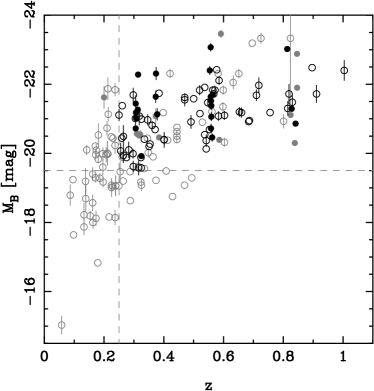
As the multi-object spectroscopy limits the number and minimum separation of targets, the observed galaxies are rather sparsely sampled. As shown in Fig. 1, the preference for cluster galaxies does therefore not significantly extend nor bias the parameter space inhabited by the cluster galaxies with respect to that of the field galaxies. It merely means that cluster galaxies are slightly over-represented compared with a purely magnitude limited sample. We can therefore internally evaluate the difference between cluster and field galaxies over a range of redshifts, using galaxies that have been selected, observed and analysed in an essentially identical manner. We have no need to resort to comparisons with other studies, and hence avoid the systematic differences this could potentially involve.

The redshift distributions of our sample galaxies are shown in Fig. 2. Clearly the number of galaxies selected which actually lie in the targeted cluster varies considerably between the observed fields. This is primarily a consequence of variation in the spiral population of the clusters, and differing availability of a priori redshifts during the target selection. Note that the shorter exposure time required for MS0440 meant we could use three masks, compared with two for the other clusters. The low numbers of selected cluster galaxies, although unfortunate, does go some way to demonstrate the extent to which we have endeavoured to keep our sample unbiased.

In order to best observe the galaxy kinematics, the slits were individually tilted to align with the major axes of the target galaxies. Tilting the slits reduces the effective spatial resolution, and so multiple masks, with different position angles on the sky, are required to accommodate all galaxy position angles. We generally used two, orthogonally aligned, masks for each field, and thus a nominal limiting slit tilt of . From previous work we have found that useful spectra can be obtained using slits tilted up to this limit. However, on occasion the limit was exceeded, principally in order to observe the same object in both masks for comparison. For the three MS0440 masks the same tilt limit was applied to maximise the number of high priority targets which could be fit in the masks. In the completed designs of the 11 masks (not including MS1054), slits were assigned to targets, including stars (roughly three per mask) for the purposes of alignment and measuring the seeing.
3 Data
3.1 Photometry
The photometry used in this study is primarily from the HST archive and our own FORS2 -band imaging. These are supplemented with additional reduced and zero-point calibrated ground-based data, kindly provided by Dr. Ian Smail, in order to provide colour information. This additional colour information is advantageous for constraining the galaxy SED and hence improving the -correction. The photometric zero-points for our -band imaging were established by matching the magnitudes of point-sources with those measured on the overlapping -band ( or ) HST images. In one case (CL0054) no -band HST data were available, and an interpolation between and magnitudes was calibrated using synthetic SEDs and used instead. This was also checked using and -band ground-based data, which gives a consistent zero-point. The mean zero-point error on the -band magnitudes is mag, adequate for our purposes. The zero-point errors are included in the overall magnitude errors. Table 5 gives the bands in which magnitudes were measured for each galaxy in our full TFR sample (as defined later).
The galaxy magnitudes were measured using SExtractor (Bertin & Arnouts, 1996). The AUTO (Kron-style) aperture was used to measure magnitudes on the original images, while colours were determined from 3 arcsec diameter aperture magnitudes measured on images which had been degraded to match the worst seeing for each field. Magnitudes and colours were corrected for Galactic extinction using the maps and conversions of Schlegel, Finkbeiner & Davis (1998).
The conversion from apparent magnitudes to absolute rest-frame -band was achieved by the following procedure. First all colour information was used to find the best fitting SED from a grid of 26, spanning types E/S0 to Sdm. These were formed by interpolating the SEDs of Aragón-Salamanca et al. (1993) and redshifting appropriately. A confidence interval on the SED was also determined by examining the of the colour fits. In cases where no colour information was available an average value and confidence interval were adopted for the SED, determined from those galaxies with available colours. The magnitude in the observed band closest to rest-frame was then adjusted by a colour- and -correction calculated from the best-fitting SED. The observed band used as the basis for the conversion is indicated in Table 5. Errors were assigned to this correction corresponding to the SEDs bounding the confidence interval determined above. Finally this magnitude was adjusted by the distance modulus of the galaxy assuming the concordance cosmology.
Because of the varying imaging available for each galaxy, we need to address concerns that for our cluster galaxies may be systematically biased with respect to the field galaxies; for example, due to different colours being available to determine the SED. Our additional imaging tends to be centred on the cluster and, particularly for the HST imaging, often has a smaller field-of-view than the -band images from which we selected the targets. Cluster galaxies will tend to be located towards the centre of the field-of-view (although this may not be so true for the star-forming spirals in our sample, particularly given that we are confined to a clustercentric radius of Mpc). We might thus expect cluster galaxies to have imaging available in more bands. However, on average we have a magnitude measured in and bands for cluster and field galaxies respectively, so there is no evidence for a difference in the number of colours available. Another concern may be that the apparent magnitude used as a basis for is measured on HST images more often for cluster galaxies than for field galaxies. The opposite is actually the case, ()% of cluster galaxies have based on HST imaging, compared with ()% of field galaxies. However, this is not especially significant, given the Poisson errors. These tests imply that any significant difference measured between the cluster and field samples cannot be attributed to the heterogeneity of the imaging.
The magnitudes were additionally corrected for internal extinction (including face-on extinction of mag), following the prescription of Tully & Fouque (1985), to give the corrected absolute rest-frame -band magnitudes, , used in the following analysis.
Note that both the cosmology and internal extinction correction prescription were chosen to allow straightforward comparison with other recent studies.
Inclinations and photometric scalelengths for the disc components of the observed galaxies were measured by fitting the galaxies with bulge+disc models using the gim2d software developed by Simard et al. (2002). This was done in all available imaging as a consistency check, and all the fits were inspected to determine the (infrequent) occasions where gim2d failed to correctly fit the data.
The inclinations, , used in this study are generally those measured in the HST images by gim2d. For galaxies without HST imaging, or with no acceptable HST fits, the best available inclination, from ground-based gim2d fits or SExtractor axial ratios was used. These supplemental inclinations were examined for biases, using a set of galaxies with both HST and ground based measurements, and corrected to match the HST gim2d values. Errors on the inclinations were estimated from the scatter in values derived from different images and methods.
Photometric disc scalelengths, , were derived from gim2d fits, preferentially on HST imaging, but also on ground-based images if HST fits were not available. Only bands near to were used to reduce any contamination due to a potential variation in scalelength with observed wavelength (e.g. de Jong, 1996). A bias with respect to rest-frame wavelength may remain, but does not affect this study significantly. Scalelengths are given in kpc, calculated assuming the concordance cosmology. The final two columns in Table 5 indicate whether the inclinations and photometric disc scalelengths were measured on HST or ground-based imaging.
Many of our photometric disc scalelengths are necessarily measured on ground-based images, often with seeing arcsec FWHM. At the angular scale is kpc arcsec-1 in our adopted cosmology. For our sample is typically kpc, and thus the FWHM of the disk surface brightness profile is kpc. This is a comparable scale to the seeing, making the measurement of difficult. For a single-component surface brightness we would expect the gim2d measurement of to be reliable, although sensitive to the precision of the seeing determination. However, with a more complicated, realistic surface brightness profile, being fit by two-component model, the limited resolution makes measurement of the disk scalelength potentially unreliable. This problem becomes significantly worse for higher redshifts and smaller galaxies. We therefore prefer not to base any inferences upon our measurements and do not consider them further in this paper, except in rough comparisons of the cluster and field parameter distributions, and as an aid to the emission line quality control procedure described in the following section.
3.2 Spectroscopy
The multi-slit spectroscopy for this study was observed using the MXU11footnotemark: 1 mode of FORS2 on the VLT. In this mode slits are cut into a mask which is then placed in the light path. This has significant advantages over the movable slits of MOS11footnotemark: 1 mode. Variable slit lengths and tilt angles give increased flexibility for the mask design, increasing the number of objects observable in a single exposure and allowing consistent alignment of the slits with the galaxy major axes. Our observations are summarized in Table 2. The seeing, as measured from stellar spectra in the masks, was typically arcsec, and always less than arcsec. The setup was similar to that used for the earlier MS1054 observations (an additional 2 masks), the only changes being a larger CCD detector and a different grism (600RI) with a substantially higher throughput. These differences give a wider wavelength coverage, although with a slightly lower spectral resolution, meaning more emission lines were observed for each galaxy in the present study.
| Cluster-field | No. of masks | Exp. time (mins/mask) |
|---|---|---|
| MS0440 | 3 | 57, 45, 30 |
| AC114 | 2 | 75 |
| A370 | 2 | 90 |
| CL0054 | 2 | 150 |
| MS2053 | 2 | 150 |
| MS1054 | 2 | 210 |
Our spectroscopic data were reduced in the usual manner (Milvang-Jensen 2003; Bamford thesis in preparation), using pyraf333PyRAF is a product of the Space Telescope Science Institute, which is operated by AURA for NASA. to script standard iraf tasks and our own routines, producing straightened, flat-fielded, wavelength-calibrated and sky-subtracted 2d-spectra. The main emission lines observed were [OII], H and [OIII], with H but no [OII] for nearby galaxies. Emission lines were identified by eye and small regions of the spectra containing each line extracted. The continuum emission was subtracted from each of these small images, which were then cropped further to produce ‘postage stamps’ of each line. In the slits (still not including the MS1054 observations), separate spectra were identified. Of these are identifiable as galaxies with emission lines. Note that from the serendipitously observed galaxies, only field galaxies that happened to be well aligned with the slit, and met all the other criteria, have been included in the TFR study.
In order to measure the rotation velocity () and emission scale lengths () we fit each emission line independently using a synthetic rotation curve method based on elfit2d by Simard & Pritchet (1998, 1999), and dubbed elfit2py444The main differences between the method of Simard & Pritchet (1999) (elfit2d) and that used here (elfit2py) are a spectral oversampling to reduce the velocity ‘quantisation’ found by Milvang-Jensen (2003), the use of an error image rather than a constant noise level, improving performance in the vicinity of skyline residuals, and the addition of a test to judge when convergence has been achieved.. In this technique model emission lines are created for particular sets of parameters, and compared to the data to assess their goodness-of fit. The model emission lines are created assuming a form for the intrinsic rotation curve, an exponential surface-brightness profile, and given the galaxy inclination, seeing and instrumental profile. The intrinsic rotation curve assumed here is the ‘universal rotation curve’ (URC) of Persic & Salucci (1991), with a slope weakly parametrized by the absolute -band magnitude, . Adopting a flat rotation curve leads to values of km s-1 lower, but does not affect the conclusions of this study. As well as and , the emission line flux, constant background level and, in the case of [OII], the doublet line ratio, are simultaneously fit.
A Metropolis algorithm (Metropolis et al. 1953, as described by Saha & Williams 1994) is used to search the parameter space to find those which best fit the data, and to determine confidence intervals on these parameters. Images of model lines with the best-fitting parameters are also produced for comparison with the data.
While there may be some concerns about the Metropolis algorithm finding a local, rather than global, minimum, inspection of the time series of accepted points in the Metropolis search shows that the and parameters converge fairly quickly to their final values, and are usually stable around these values for the remainder of the sampling iterations. This implies fairly deep and smooth global minima in chi-squared space, with few local minima.
In contrast, the less well constrained, but also less critical, parameters of background level and doublet ratio show more frequent jumps between semi-stable values. While this reveals the existence of local minima, it also demonstrates the algorithm’s ability to move out of such regions when they exist. The final error in the measured parameter thus includes the uncertainty due to the multiplicity of chi-squared minima. The jumps between minima in these subsidiary parameters are rarely accompanied by any significant shift in the stable and parameter values.
Two of the emission line galaxies do not have absolute -band magnitudes from the photometry, and a further four have no lines suitable for fitting (i.e. the lines were so faint that the mean flux across the postage stamp was negative due to the noise). An additional galaxies were discarded due to their inclinations being deemed highly uncertain. For the remaining objects, a mean of suitable lines per galaxy were fit by the procedure described above.
The principal results of the rotation curve fitting are measurements of and with estimates of their error for, in general, several emission lines per galaxy. (Actually is measured, which is converted to , using the inclinations described in §3.1, once an average value of has been determined for each galaxy.) In order to produce a single value of and for each galaxy the values for the individual lines (labelled by below) are combined by a weighted mean. Upper and lower errors () on these average parameters are determined as the maximum of (a) a weighted combination of the individual errors estimated by elfit2py, and (b) the standard error of the weighted mean determined from the individual measurements. For example, with weights
| (1) |
the computed upper error on the average is the square-root of
where is the number of measurements contributing to the average. The first term in the function corresponds to case (a) above, and the second to case (b). The lower error is computed similarly.
For most galaxies the error calculated from those given by elfit2py is close to that inferred from the standard error of the data, and hence case (a) applies, or case (b) causes a negligible increase in the error. However, for galaxies where there is inconsistency between values from different lines, and no way of determining which lines should be preferred, case (a) would underestimate the true uncertainty. In these situations case (b) provides a more realistic estimate of the error. This test is obviously not possible for galaxies with only one observed (and accepted by the quality control procedure) emission line, and therefore will cause formally inconsistent errors. However, this is judged to be a minor problem when compared with the elimination of occasional situations where the uncertainty would otherwise be seriously underestimated.
A significant fraction of the emission lines identified display dominant nuclear emission, or asymmetries in intensity, spatial extent or kinematics. In severe cases these departures from the assumed surface brightness profile and intrinsic rotation curve mean that the best-fitting model is not a true good fit to the data. A similar situation can occur for very low signal-to-noise () lines, where an artifact of the noise overly influences the fit. More concerning is the case of very compact lines, where the number of pixels is on the order of the number of degrees of freedom in the model, and hence an apparently good fit is obtained despite a potentially substantial departure from the assumed surface brightness profile.
In order to eliminate such ‘bad’ fits a number of quality tests are imposed, based on a measure of the median (per pixel over the region where the model line has significant flux), and a robust reduced- goodness-of-fit estimate (). The cuts on these quantities were set following a detailed simultaneous inspection of the data, model line and best-fitting parameters. Firstly, for each line a lower limit in is applied, followed by an upper limit on . As an initial attempt at excluding sources too compact to fit reliably, lines were also rejected if the best-fitting scalelength of the emission was consistent with zero within the confidence interval derived by elfit2py.
These cuts alone were deemed too inefficient, i.e. cuts rejecting all obviously ‘bad’ fits resulted in an excessive number of clearly ‘good’ fits being discarded. Ideally we would prefer an entirely quantitative method, and therefore a number of additional quantities were calculated to assist the quality judgement. The line was fit by a Gaussian in each spatial row555using the iraf/stsdas task ngaussfit, with the errors on each Gaussian fit determined by repeated simulations with different noise realisations corresponding to the error image. It was found that for the [OII] doublet, fitting a single Gaussian was more robust than attempting to simultaneously fit both components. Through inspection of the parameters and their errors quantitative criteria were developed for judging whether the fit position is reliable. The emission line was thus ‘traced’ and the region determined for which the trace is reliable.
The distance from the continuum centre to where the line could no longer be reliably detected above the noise we term the extent (). This quantity is dependent on the properties of the data, e.g. pixel size and seeing, and is thus not suitable for comparison with other studies. However, it is useful for the internal investigation of differences between various subsets of our own data set. Note that elfit2py uses all the pixels simultaneously, and therefore successfully uses information further out than when fitting a model line. Indeed, reasonable fits can be obtained even with lines for which is zero.
Additional quantities describing the asymmetry, in terms of extent and kinematics, and the flatness of the line at maximum extent were also formulated. However, a satisfactory set of criteria based on these quantities could not be found. Therefore, with the above cuts on and established all of the model lines were reviewed by eye, along with the galaxy images, observed emission line, model parameters and the various quantities just described. From this inspection lists were compiled of those lines to be unconditionally excluded or included in the calculation of . The main occasions where such action was necessary was to exclude lines which were clearly due to very central emission, judged in combination with the ratios and , but where was low enough to make the adopted cut.
Also unconditionally excluded were lines which made the and cuts, but were obviously incorrect or clearly inconsistent with other lines available for the galaxy, particularly when this was for an obvious reason such as low or interference from skyline residuals. The primary cases for unconditional inclusion were where slight asymmetries and/or absorption wings caused a high value, but the fit was clearly well matched to a high line with large and .
After the application of these visual exclusions and inclusions, any galaxy with an average consistent with zero rotation, within the errors given by Eqn. 3.2, was discarded from the sample. While this is not ideal, it is very useful to remove galaxies for which the emitting region is probably not rotationally supported. The above line selections were then re-applied with the additional constraint that individual lines were also rejected if their best-fitting was consistent with zero within the confidence interval derived by elfit2py.
In five cases there are two spectra corresponding to the same galaxy, both intentionally, for comparison purposes, and coincidentally. In one case the second observation is with a slit at a angle to the major axis of the galaxy and thus of much lower quality. This observation was therefore discarded. The remaining four galaxies have reasonably consistent measured parameters from their duplicated spectra and thus weighted averages of the fit parameters are adopted.
After the rigorous line quality-control procedure, galaxies remain. These comprise the TFR sample of the five cluster fields observed for this study. In order to consistently combine the MS1054 data with this sample, the emission line postage stamps for the MS1054 galaxies have been re-fit using elfit2py and the same line quality criteria applied. Of the galaxies with emission in the MS1054 observations, remain after applying the line quality criteria. These are added to the sample described above, giving a total of galaxies, with a mean of lines contributing to the measurements for each galaxy.
3.3 Data table
The data described above are presented in Table 3. The first four columns give the ID assigned in this study, the R.A. and Dec. in J2000 coordinates and the redshift (). Column 5 (labelled ‘Mem.’) indicates whether each galaxy is a cluster member according to the criteria used in this paper, ‘F’ and ‘C’ indicate field and cluster respectively. The galaxy inclination is given in column 6 (), with corresponding to edge-on, and column 7 () lists the internal extinction corrections applied (including 0.27 mag of face-on extinction), with errors corresponding to the uncertainty in the measured inclination. Column 8 gives the absolute rest-frame -band magnitude () in our assumed cosmology (, , km s-1 Mpc-1), corrected for Galactic and internal extinction, with errors including the contributions from the initial measurement and all subsequent corrections. Column 9 specifies the rotation velocity () for each galaxy, derived from elfit2py, averaged over all lines which pass the quality control criteria. The errors on this quantity include those determined via Eqn. 3.2, combined with the error on the correction from to . Finally, column 10 gives the weight () assigned to each galaxy in the TFR fits of Eqn. 5 in §5. Only galaxies in the matched samples, defined below in §4, are included in these TFR fits, and therefore only these galaxies have values.
| ID | R.A. | Dec. | Mem. | ||||||
|---|---|---|---|---|---|---|---|---|---|
| [J2000] | [J2000] | [deg] | [mag] | [mag] | [dex] | ||||
| MS0440_101 | 04 43 14.6 | 02 05 49 | F | 0.017 | |||||
| MS0440_140 | 04 43 09.0 | 02 06 13 | F | 0.014 | |||||
| MS0440_188 | 04 43 19.3 | 02 06 42 | F | 0.004 | |||||
| MS0440_207 | 04 43 16.8 | 02 07 01 | F | – | |||||
| MS0440_273 | 04 43 16.4 | 02 07 31 | F | 0.018 | |||||
| MS0440_311 | 04 43 06.2 | 02 07 51 | F | 0.011 | |||||
| MS0440_319 | 04 43 07.8 | 02 08 06 | F | – | |||||
| MS0440_538 | 04 43 18.1 | 02 09 43 | F | – | |||||
| MS0440_616 | 04 42 58.8 | 02 09 37 | F | – | |||||
| MS0440_627 | 04 43 14.9 | 02 09 33 | F | 0.019 | |||||
| MS0440_635 | 04 43 27.2 | 02 09 43 | F | – | |||||
| MS0440_657 | 04 42 50.5 | 02 09 45 | F | 0.014 | |||||
| MS0440_735 | 04 43 07.2 | 02 10 21 | F | – | |||||
| MS0440_849 | 04 43 14.4 | 02 10 30 | F | 0.016 | |||||
| MS0440_1109 | 04 43 05.9 | 02 10 45 | F | – | |||||
| MS0440_1131 | 04 43 06.7 | 02 12 15 | F | 0.018 | |||||
| MS0440_1157 | 04 43 10.9 | 02 11 32 | F | 0.017 | |||||
| AC114_115 | 22 58 59.7 | -34 50 52 | F | 0.020 | |||||
| AC114_264 | 22 58 55.1 | -34 49 49 | F | – | |||||
| AC114_391 | 22 58 45.6 | -34 49 03 | F | 0.021 | |||||
| AC114_553 | 22 58 56.7 | -34 48 18 | F | – | |||||
| AC114_700 | 22 58 33.7 | -34 47 43 | F | 0.019 | |||||
| AC114_810 | 22 58 46.1 | -34 46 00 | F | 0.014 | |||||
| AC114_875 | 22 58 51.2 | -34 46 21 | F | – | |||||
| A370_39 | 02 39 48.1 | -01 38 16 | F | – | |||||
| A370_119 | 02 40 02.5 | -01 37 13 | F | 0.019 | |||||
| A370_157 | 02 39 55.5 | -01 36 59 | F | 0.018 | |||||
| A370_183 | 02 40 00.4 | -01 36 38 | F | 0.017 | |||||
| A370_210 | 02 40 00.9 | -01 36 16 | F | – | |||||
| A370_292 | 02 39 57.8 | -01 35 49 | F | 0.013 | |||||
| A370_319 | 02 39 51.8 | -01 35 21 | F | 0.008 | |||||
| A370_401 | 02 39 54.5 | -01 35 04 | F | 0.018 | |||||
| A370_406 | 02 40 13.9 | -01 35 05 | F | 0.015 | |||||
| A370_540 | 02 40 09.7 | -01 32 05 | F | – | |||||
| A370_582 | 02 40 10.5 | -01 33 29 | F | – | |||||
| A370_620 | 02 40 04.3 | -01 32 59 | F | 0.020 | |||||
| A370_630 | 02 39 50.3 | -01 34 22 | F | – | |||||
| A370_650 | 02 39 57.8 | -01 33 10 | F | 0.014 | |||||
| A370_751 | 02 39 57.5 | -01 34 32 | F | 0.020 | |||||
| CL0054_62 | 00 57 00.9 | -27 44 18 | F | 0.017 | |||||
| CL0054_83 | 00 56 52.4 | -27 44 06 | F | 0.020 | |||||
| CL0054_89 | 00 56 52.4 | -27 44 04 | F | 0.017 | |||||
| CL0054_126 | 00 56 59.3 | -27 43 41 | F | – | |||||
| CL0054_137 | 00 56 55.7 | -27 43 25 | F | 0.016 | |||||
| CL0054_138 | 00 56 46.3 | -27 42 50 | F | – | |||||
| CL0054_284 | 00 56 55.7 | -27 42 17 | F | 0.017 | |||||
| CL0054_354 | 00 57 02.3 | -27 41 31 | F | – | |||||
| CL0054_407 | 00 57 00.7 | -27 41 05 | F | 0.015 | |||||
| CL0054_454 | 00 57 09.9 | -27 40 44 | F | 0.020 | |||||
| CL0054_579 | 00 57 12.3 | -27 40 14 | F | 0.015 | |||||
| CL0054_588 | 00 57 09.1 | -27 40 27 | F | 0.013 | |||||
| CL0054_686 | 00 56 50.9 | -27 38 01 | F | 0.010 | |||||
| CL0054_688 | 00 56 53.8 | -27 37 14 | F | 0.020 | |||||
| CL0054_779 | 00 57 14.5 | -27 38 04 | F | 0.015 | |||||
| CL0054_803 | 00 56 57.6 | -27 38 24 | F | – | |||||
| CL0054_827 | 00 57 09.1 | -27 38 36 | F | 0.019 | |||||
| CL0054_892 | 00 56 55.6 | -27 39 08 | F | 0.008 | |||||
| CL0054_927 | 00 57 07.9 | -27 39 28 | F | 0.016 | |||||
| CL0054_937 | 00 56 56.8 | -27 39 34 | F | 0.015 | |||||
| CL0054_979 | 00 56 47.2 | -27 38 33 | F | 0.019 | |||||
| CL0054_993 | 00 57 11.4 | -27 39 46 | F | – |
| ID | R.A. | Dec. | Mem. | ||||||
|---|---|---|---|---|---|---|---|---|---|
| [J2000] | [J2000] | [deg] | [mag] | [mag] | [dex] | ||||
| CL0054_1011 | 00 56 58.9 | -27 40 20 | F | – | |||||
| CL0054_1054 | 00 56 59.8 | -27 38 08 | F | 0.018 | |||||
| MS2053_86 | 20 56 12.4 | -04 38 26 | F | – | |||||
| MS2053_371 | 20 56 17.8 | -04 38 01 | F | 0.017 | |||||
| MS2053_404 | 20 56 18.7 | -04 37 07 | F | 0.022 | |||||
| MS2053_435 | 20 56 18.9 | -04 40 04 | F | 0.021 | |||||
| MS2053_455 | 20 56 20.0 | -04 35 54 | F | – | |||||
| MS2053_470 | 20 56 19.5 | -04 38 47 | F | 0.020 | |||||
| MS2053_741 | 20 56 23.2 | -04 34 41 | F | 0.019 | |||||
| MS2053_856 | 20 56 24.8 | -04 35 34 | F | 0.021 | |||||
| MS2053_998 | 20 56 22.6 | -04 41 32 | F | – | |||||
| MS2053_1105 | 20 56 29.6 | -04 38 08 | F | – | |||||
| MS2053_1296 | 20 56 34.2 | -04 38 02 | F | – | |||||
| MS1054_F02 | 10 56 48.3 | -03 37 33 | F | – | |||||
| MS1054_F04 | 10 56 56.0 | -03 37 28 | F | – | |||||
| MS1054_F05 | 10 57 01.3 | -03 35 44 | F | – | |||||
| MS1054_F06 | 10 56 53.0 | -03 38 41 | F | 0.021 | |||||
| MS1054_F08 | 10 57 08.2 | -03 37 34 | F | – | |||||
| MS1054_F10 | 10 57 12.3 | -03 37 17 | F | 0.019 | |||||
| MS1054_F11 | 10 57 08.2 | -03 36 42 | F | 0.021 | |||||
| MS1054_F12 | 10 57 11.5 | -03 36 44 | F | 0.021 | |||||
| MS1054_F14 | 10 56 54.7 | -03 39 00 | F | – | |||||
| MS1054_F16 | 10 57 01.2 | -03 34 20 | F | 0.021 | |||||
| MS1054_F18 | 10 57 03.7 | -03 38 33 | F | 0.021 | |||||
| MS1054_F19 | 10 56 50.7 | -03 35 39 | F | 0.019 | |||||
| MS1054_F20 | 10 57 05.7 | -03 36 26 | F | 0.020 | |||||
| MS1054_F21 | 10 56 48.6 | -03 35 42 | F | 0.019 | |||||
| MS1054_F22 | 10 57 07.8 | -03 37 04 | F | 0.022 | |||||
| AC114_18 | 22 58 48.5 | -34 51 39 | C | 0.048 | |||||
| AC114_142 | 22 58 52.0 | -34 50 42 | C | 0.047 | |||||
| AC114_193 | 22 58 58.9 | -34 50 20 | C | 0.053 | |||||
| AC114_768 | 22 58 35.8 | -34 45 47 | C | 0.049 | |||||
| AC114_930 | 22 58 34.0 | -34 46 52 | C | 0.028 | |||||
| AC114_959 | 22 58 49.3 | -34 47 01 | C | 0.039 | |||||
| AC114_1001 | 22 58 30.1 | -34 47 21 | C | 0.036 | |||||
| A370_532 | 02 39 51.0 | -01 32 12 | C | 0.051 | |||||
| A370_538 | 02 39 58.2 | -01 32 32 | C | 0.050 | |||||
| A370_555 | 02 39 46.4 | -01 32 17 | C | 0.050 | |||||
| CL0054_358 | 00 57 04.5 | -27 41 30 | C | 0.037 | |||||
| CL0054_609 | 00 56 45.2 | -27 38 08 | C | 0.049 | |||||
| CL0054_643 | 00 56 45.4 | -27 38 06 | C | 0.040 | |||||
| CL0054_714 | 00 56 46.2 | -27 37 23 | C | 0.044 | |||||
| CL0054_725 | 00 56 44.8 | -27 37 46 | C | 0.051 | |||||
| CL0054_799 | 00 56 56.4 | -27 38 22 | C | 0.049 | |||||
| CL0054_860 | 00 56 49.6 | -27 38 51 | C | 0.049 | |||||
| CL0054_918 | 00 57 05.5 | -27 40 04 | C | 0.044 | |||||
| CL0054_966 | 00 56 48.4 | -27 40 03 | C | 0.037 | |||||
| MS1054_C01 | 10 57 12.0 | -03 36 50 | C | 0.050 | |||||
| MS1054_1403 | 10 57 03.8 | -03 37 43 | C | 0.053 | |||||
| MS1054_2011 | 10 57 07.1 | -03 35 40 | C | 0.048 |
4 ‘Matched’ cluster and field samples
Cluster membership has been assigned based on redshifts and velocity-dispersions from the literature (Girardi & Mezzetti, 2001; Stocke et al., 1991; Hoekstra et al., 2002). These are given in Table 1, along with the corresponding redshift limits we have adopted (). In each field, galaxies with are considered to be cluster members.
Our target selection has been performed in a way designed to give easily comparable samples of field and cluster galaxies, however further efforts are required to ensure these samples are well matched. While the cluster galaxies are located at particular redshifts, between , the field galaxies span a much wider range in redshift, and consequently in absolute magnitude. As the TFR may evolve with redshift, irrespective of environment (e.g. see Paper 2), care must be taken to avoid this complicating the comparison between cluster and field. In particular, the evolution of low-luminosity galaxies, which are not represented in our sample at higher redshifts, is particularly unconstrained. We therefore impose cuts of and mag, simply chosen to better match the distribution of field galaxies to that of the cluster sample, as indicated in Fig. 3.
The ‘matched’ TFR sample used for the clusterfield comparison in this paper thus contains a total of galaxies, comprising field and cluster galaxies.
Now we have established samples of field and cluster galaxies over similar epochs and luminosity ranges, we can investigate whether the samples differ in other ways. The distributions of , , and are shown in Fig. 1, with the K-S test confidence levels that the parent distributions of the two samples are the same. Note from Figures 1(a) and 3 that the cluster and field galaxies cover a very similar range in , with a hint that the cluster galaxies extend to brighter magnitudes. There should be absolutely no difference in the selection of galaxies at the bright end of this distribution. This is therefore a first indication that cluster spirals may be brighter than those in the field.
The distributions of galaxy size, in terms of both photometric and spectroscopic scalelength (Fig. 1 panels (b) and (d)), are similar for the field and cluster samples. For they are practically identical, although it is worth noting that the cluster members do extend to larger values. On the other hand, the cluster distribution is restricted to lower values than the field.
The two samples cover the same range in , although there is evidence that the cluster galaxies have a slightly broader distribution, possibly more skewed to lower values. This is considered further in the discussion (§6). However, these differences are minor, and point at real characteristics of the galaxy population, rather than a selection bias.
5 Cluster versus field TFR
Fig. 4 shows the TFR for our ‘matched’ samples of field and cluster galaxies. A fiducial local field TFR is indicated by the thin lines. This is derived from the TFR of Pierce & Tully (1992, hereafter PT92), with a zero-point adjustment because PT92, while otherwise using the internal extinction correction of Tully & Fouque (1985), do not include the mag of face-on extinction that is applied to our data. The fiducial PT92 TFR, adapted to our internal extinction correction, is thus:
| (3) |
The thick solid line in Fig. 4 is a fit to the matched field sample. This is a weighted, least-squares fit, minimising the residuals in (referred to as an ‘inverse’ TFR fit) and incorporating an intrinsic scatter term, as described in more detail in Paper 2. The thick dotted and dashed lines are fits to the cluster sample, performed by the same method, except for the dashed line the slope was fixed to that of the fit to the matched field sample. The fit to the matched field sample, and cluster samples with free and fixed slopes, respectively give
| (4) | |||||
The slope of the fit to the cluster sample is markedly shallower than that to the matched field sample. However, the slopes only differ by , so this not a significant result.
The weights () assigned to each galaxy in the above fits are given in Table 3. These are calculated from the reciprocal of the sum of the squared uncertainties in and and the intrinsic scatter. The best fit is determined iteratively, because of its dependence on the slope (used to convert the error into one in ) and intrinsic scatter. The only differ by between the two alternative cluster fits; the values for the free-slope fit are given.
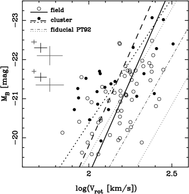
It can be seen that the field galaxies lie primarily along a reasonably tight relation, with similar slope to the local fiducial TFR, but with an offset to brighter magnitudes and/or lower rotation velocities. This is particularly clear when considering the full field sample, unrestricted in , as in Paper 2. This overall, systematic offset from the fiducial local TFR is of little concern for this study. As discussed more thoroughly in Paper 2, a comparison with the intercept of the PT92 TFR must consider the different manners in which the magnitudes and rotation velocities are measured for the two studies. It is also likely that the absolute calibration of the PT92 TFR is incorrect by mag, as discussed further in Paper 2. Correcting for this would bring the fiducial TFR into closer agreement with our field sample, particularly for the low redshift objects.
The cluster members are preferentially located above the field relation, particularly for galaxies with lower rotation velocities km s-1, as also indicated by the shallower slope of their TFR fit. To help compare the field and cluster samples we can take out the slope and examine the residuals from the fiducial TFR:
| (5) | |||||
The difference between the cluster and field galaxies is particularly evident in a histogram of , as shown in Fig. 5(a). The peaks of the distributions are clearly not aligned, such that cluster galaxies are generally brighter at a fixed rotation velocity. A K-S test gives the probability of the parent distributions being the same as %.
To assess this offset more quantitatively we can consider the mean and variance of for each of the samples. These are calculated in a similar manner to the TFR fitting method described in Paper 2. Weighted means and variances are calculated, with weights assigned from the measurement errors in combination with an iteratively-determined intrinsic scatter. The derived offset between the cluster and field samples is mag. A -test gives the significance of this offset as .


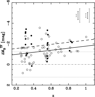
It could be suggested that the offset we find between field and cluster galaxies is due to the combination of a general (field) trend with redshift and a difference between the redshift distribution of the field and cluster samples. In order to demonstrate that this is not the case we plot versus redshift in Fig. 6. Despite a possible trend in with redshift for the field population, as examined in Paper 2, the offset is clearly still present, with cluster galaxies consistently brighter for the same rotation velocity and redshift. The best-fitting field evolution from Paper 2 is
| (6) |
Subtracting this field evolution does not change either the size or significance of the clusterfield offset. This can also be seen in Fig. 5(b), a histogram of with the field evolution taken out, although the K-S significance declines slightly.
Note that we have selected cluster galaxies in each field simply from their redshifts coinciding with the targeted clusters. It is possible that a number of the galaxies we classify here as ‘field’ actually reside in separate high density regions. Unfortunately, our sample is not large enough to identify additional groups in our field. It will be interesting to see if the field scatter is reduced in future studies, when such groups can be excluded, and whether the group spirals inhabit the same region of the TFR as our cluster sample.
6 Discussion
6.1 Origin of the TFR clusterfield offset
It is clear that there is a significant difference between the cluster and field galaxies in our sample. As the galaxies have all been selected, observed and analysed in the same manner, it is very likely this difference is real. Now we must consider the reasons for this disparity. The offset from the field TFR may be due to some effect causing cluster galaxies to appear brighter for a given rotation velocity, slower-rotating for a given magnitude, or a combination of both. Physically, both scenarios are possible, an enhancement of star-formation would lead to a brightening, while stripping of the dark matter halo by the cluster potential could, at least hypothetically, decrease the galaxy mass and hence lower .
Simulations by Gnedin (2003b, hereafter G03b) find that changes little (% decrease), even when over half of a galaxy’s dark-matter halo is stripped away. This is because the halo is truncated to a galactocentric radius that lies beyond the edge of the luminous disk. Within the region that the galaxy is luminous – and thus its rotation can be measured – the halo is mostly unaffected, the enclosed mass stays constant, and therefore remains the same.
G03b uses a pseudo-isothermal initial dark matter density profile. This is ‘cored’ (finite at the centre), as opposed to the ‘cuspy’ halo profiles generally produced by CDM simulations (Navarro et al., 1996; Moore et al., 1998). However, cored profiles (van Albada et al., 1985; Burkert, 1995) seem to be required for galaxy haloes, from observations of individual rotation curve shapes (e.g. Gentile et al., 2004), and in order to solve the problem of reproducing the TFR zeropoint in a hierarchical universe (Navarro & Steinmetz, 2000). If galaxy haloes are instead actually cuspy, it would be even harder to remove dark matter from their inner regions than found by G03b. From this point of view their result provides an upper limit on the feasible change in due to tidal interaction with a cluster.
However, higher resolution simulations using a different code, also performed by G03b, find slightly larger decreases in of %. Adopting the slope of the PT92 TFR, this corresponds to an apparent brightening at fixed rotation velocity of mag, comparable to the TFR offset we measure.
In addition, the G03b simulations discussed above are based on galaxies with km s-1. Less massive galaxies, with correspondingly less dense haloes, may well be more seriously affected. For example, G03 find that low surface brightness galaxies with comparable masses, but much more extended haloes, suffer decreases in of %, while dwarf galaxies, with initial km s-1, are completely destroyed. This could explain why most of our cluster galaxies with large TFR offsets have low rotation velocities, km s-1. Further simulations would be helpful to establish how the effectiveness of tidal stripping depends upon the initial rotation velocity of infalling galaxies.
With our present data, and the uncertainties concerning the dark matter halo profile, we therefore cannot exclude tidal stripping of the galaxy dark matter haloes as an origin for the cluster–field TFR offset we measure.
The enhanced SFR hypothesis is supported by the increased fraction of galaxies with strong E+A spectra (EW(H) Å) in intermediate redshift clusters (Poggianti et al., 1999; Tran et al., 2003), implying these galaxies have recently experienced a short star-burst prior to truncation of their star-formation. More direct evidence is provided by a correlation between star-formation rate and offset from the fiducial TFR, as suggested by our MS1054 sample in Milvang-Jensen (2003) and Milvang-Jensen & Aragón-Salamanca in preparation, and which will be the subject of further study using our entire TFR sample.
However, there may be a less straightforward reason why we observe lower rotation velocities for cluster galaxies. This could be a symptom of cluster galaxies having rotation curves or emission surface brightness profiles that are different from field galaxies. Both of these could cause a systematic divergence from the assumptions used in elfit2py, thereby affecting the measured value of . Vogt et al. (2004) find spirals in local clusters with truncated H emission and deficient in HI, presumably due to removal of gas from the outer regions of the disc through interactions with the cluster environment. If spirals in our cluster sample are significantly affected by this, then we may preferentially be observing emission from nearer the centre of these galaxies. This could potentially bias our measurements to lower values. To look for any differences in the extent, quality and shape of the rotation curves between the two samples, we can utilise the emission line ‘traces’ described in §3.2.

Recall that is the spatial distance, from the line centre, to which we can reliably detect the emission above the background noise. This was determined by attempting to fit a Gaussian to the emission in each spatial row, repeating the fit with different noise realisations to determine average Gaussian parameters and their uncertainties. The sanity of these parameters and their significance, as judged by the derived uncertainties, were then used to classify each average fit as ‘good’ or ‘bad’, according to whether the emission was reliably detected in that spatial row. In addition, isolated points, otherwise deemed to be ‘good’, but separated from other ‘good’ points by more than two spatial pixels, were also judged unreliable and hence classified as ‘bad’ points. The resultant values of are thus robust measurements of the extent to which the emission lines can be reliably detected. The distributions of emission line extent, , in units of kpc, for all lines used to measure for galaxies in the ‘matched’ samples, are shown in Fig. 7. It is clear that there is very little difference between the extent of the emission lines for cluster and field galaxies, and hence no evidence of a bias that could affect the measured values of and . If anything, Fig. 7 suggests that we can actually trace the emission out further in cluster galaxies than in field galaxies.


The distributions of the additional quality assessment quantities, and are shown in Fig. 8. Again, there is no appreciable difference between the two samples, apart from a hint that the lines of cluster galaxies extend to higher than those of the field galaxies. We therefore conclude that there is no significant difference in the extent or quality-of-fit of our cluster and field galaxy rotation curves.
In addition, even if there are differences in the and distributions of our cluster and field samples, we find no correlation between and these quantities, so this cannot be responsible for the TFR offset we measure. This is demonstrated by Fig. 9, plots of the fractional deviation of the of individual lines, from the weighted mean of all the ‘good’ lines for that galaxy (), versus and . Note that the scatter increases with both decreasing and , as one would expect.


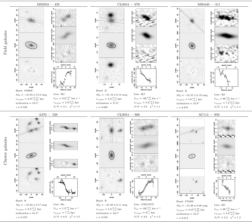
Representative examples of our data, model lines and observed rotation curves, for both field and cluster galaxies, are shown in Fig. 10. The plotted rotation curves have been measured by the tracing method described in §3.2, combined by weighted averages of the reliable points in the case of multiple lines for a single galaxy. Only points with at least one ‘good’ measurement are plotted, thereby showing the extent to which we can reliably trace the line. The model lines have been traced, and ‘good’ points determined, in exactly the same way, so that the extent of the model line shows the distance to which it can be reliably traced assuming the same pixel errors as the real data. Note that is not measured using this method, but rather by comparison with model 2D spectra in the Metropolis parameter search of elfit2py. Visually there is no difference in the form and quality of the emission lines and rotation curves between the two samples. We therefore assert that the offset between the TFR of the two samples is due to real, physical differences in and/or .
Note that the objects in our sample are giant galaxies, which must have emission lines bright enough for us to be able to fit and hence measure . Our results therefore apply to massive ( km s-1), luminous () galaxies, with significant active star-formation in the disc. No conclusions may be drawn concerning the population of fainter disc galaxies or those with little or no ongoing star-formation.
For the MS1054 sample alone, evidence for a correlation between and star-formation rate has already been demonstrated (Milvang-Jensen 2003, Milvang-Jensen & Aragón-Salamanca in preparation). This suggests that a change in due to enhanced star-formation is the main cause of the TFR clusterfield offset. More insight into this issue will be provided by future investigation of the star-formation rates for the galaxies in the present sample, combined with those from our Subaru study.
6.2 Comparison with other studies
In contrast to our result, the study of Ziegler et al. (2003) finds no difference between the TFR of spirals in three clusters at and that determined for the FORS Deep Field by Böhm et al. (2004). This is puzzling, and may point to real differences in TFR offsets between individual clusters. However, this question must wait to be addressed by larger studies which can examine TFR offsets, along with SFRs and colours, as a function of cluster properties.
It seems difficult to attribute the conflict between our results and those of Ziegler et al. (2003) to a difference in sample selection (see Jäger et al., 2004). This was performed in a fairly similar manner, generally giving preference to galaxies based on luminosity, spiral morphology, known emission lines, and cluster membership. However, both studies have rather heterogeneous selection procedures, based upon the availability of disparate prior data in the literature. Additional, higher quality data for four more clusters are expected soon from this group, which should help confirm which result is correct. We are also in the process of fitting subsamples of each others’ emission line data, in order to assess the robustness of our rotation velocities with respect to the analysis methods used.
A study of spirals in the cluster CL0024+1654 at by Metevier & Koo (2004) finds a TFR offset for their galaxies, with respect to the local field, of mag. This suggests there is little difference between cluster and field spirals at , when combined with the mag of field evolution expected at this redshift from the results of Paper 2. However, few details of their study have been published to date, and so a proper comparison with our work is not possible. Data for more clusters will be provided soon by our Subaru study (Nakamura et al. in preparation), and future work by the EDisCS collaboration.
More general studies of the correlation between SFR and local galaxy density by Lewis et al. (2002) and Gómez et al. (2003), using the 2dF and SDSS datasets respectively, both find the existence of a critical local galaxy density (of galaxy with per Mpc2). At densities greater than this, the average SFR decreases with density. At lower densities there is no significant correlation. These results imply that the global SFR of the universe may be influenced by environmental effects at quite low densities, outside of the boundaries of rich clusters, and therefore its variation is not simply due to a general, internal evolution of the SFR in individual galaxies.
How does the finding that groups may be the dominant site of star-formation suppression today compare with our result, that we also find this process occurring – accompanied by a SFR enhancement – in rich clusters at intermediate redshift? Firstly, the fact that suppression of SFR happens at low densities locally does not rule out it also occurring in cluster environments. Rather, the linearity of the SFR–density correlation implies that the efficiency of SFR suppression increases with density.
Furthermore, Balogh et al. (2004) find that the environmental dependence of the volume averaged SFR is due to changing proportions of the star-forming and passive galaxy populations, rather than a shift in the mean SFR of star-forming galaxies. This suggests that the process responsible for reducing the average SFR in groups is stochastic. When the process occurs it causes a halt in star-formation, and hence a transformation from a galaxy in the star-forming population into the passive population. However, in order to preserve the smooth correlation between SFR and local density, this process must occur randomly, with a frequency related to the local density. This suggests mergers as the responsible mechanism for SFR suppression in groups. However, in local rich clusters very few star-forming galaxies are found, yet mergers are less likely due to the large relative galaxy velocities. In this case it may be that a more all-encompassing mechanism, such as ram-pressure stripping, is at work, finishing the job started in groups.
Another finding by Balogh et al. (2004), that star-forming galaxies in dense environments have an EW(H) distribution indistinguishable from that for low-density environments, appears at first to be inconsistent with the present paper’s results. However, the necessarily short time-scale for any SFR enhancement, combined with the simultaneous existence of galaxies with declining SFR, may make detecting such an effect difficult using the EW(H) distribution.
A further explanation may be one of pre-processing. It seems likely that galaxies falling into rich clusters today have spent a longer time subjected to group conditions than those entering similar clusters at . If, as is suggested above, the probability for star-formation suppression increases with both local density and the length of time which the galaxy has been subjected to the environment, we would therefore expect clusters to be the site of star-formation truncation at intermediate redshifts, but no longer today – at least for massive galaxies, which are preferentially located in denser regions. However, to assert this will require a consideration of cosmological simulations beyond the scope of the present paper.
There has been surprisingly little direct study of the local () dependence of the TFR on environment, although this is perhaps because a lack of any dependence is apparent in more general studies. An investigation by Biviano et al. (1990) finds no evidence for a difference between the TFR of spirals in clusters and those in a sample taken from groups and the field. This provides some evidence that any difference between cluster and field spirals that may have existed in the past, has now diminished, at least for those spirals which retain significant quantities of HI. Studies of asymmetry, truncation and HI deficiency in cluster spirals have also been performed for local clusters (Dale et al., 2001; Vogt et al., 2004), finding evidence for the stripping of disc gas through some process related to galaxy infall.
The variation of galaxy properties with environment, as investigated by the studies mentioned above, suggests a similar examination of TFR offset with respect to clustercentric distance and local density for our data. We plan to undertake a such a detailed ‘geographical’ study of our VLT and Subaru intermediate-redshift clusters once the samples have been combined and further spectral properties measured. We therefore do not consider this any further in the present paper.
7 Conclusions
We have constructed the TFR for samples of homogeneously selected and analysed field and cluster spirals with and . From this we have found that cluster galaxies are offset from the field TFR by mag, such that those in clusters are over-luminous for a given rotation velocity. The reality of this offset is significant at a confidence level. This offset remains, with similar significance, even if a global evolution in the field population is taken into account. It should be stressed that this result applies only to the bright, massive, star-forming, disc galaxies which form the sample considered here. However, we do find a marginal indication that the galaxies in our sample with lower rotation velocities ( km s-1) contribute most to our measured offset.
We have extensively compared the emission lines of the field and cluster samples, finding no difference to which we could attribute the TFR offset. The most likely explanation is that the cluster galaxies have been brightened by their initial interaction with the intra-cluster medium. This is presumably due to an initial enhancement of their star-formation rate, before further interaction has suppressed it. However, at this point we cannot rule out the possibility of a change in due to stripping of the dark matter haloes of cluster galaxies. Discriminating between TFR offsets due to changes in either luminosity or rotation velocity will require further work, such as examining the difference in star-formation rate for distant cluster and field galaxies, and its correlation with TFR offset.
Acknowledgments
We would like to thank Ian Smail, for generously providing additional imaging data, and Pierre-Alain Duc, for allowing us access to an unpublished spectroscopic catalogue of CL0054 used in the target selection process. We also thank Osamu Nakamura for useful discussions, and the referee, Bodo L. Ziegler, for his detailed and helpful comments. The Simbad and VizieR services provided by the Centre de Données astronomiques de Strasbourg (CDS) were used in the course of this work.
References
- Abadi, Moore, & Bower (1999) Abadi M. G., Moore B., Bower R. G., 1999, MNRAS, 308, 947
- Aragón-Salamanca et al. (1993) Aragón-Salamanca A., Ellis R. S., Couch W. J., Carter D., 1993, MNRAS, 262, 764
- Balogh, Navarro, & Morris (2000) Balogh M. L., Navarro J. F., Morris S. L., 2000, ApJ, 540, 113
- Balogh et al. (2004) Balogh M., et al., 2004, MNRAS, 348, 1355
- Bamford et al. (2005) Bamford S. P., Aragón-Salamanca A., Milvang-Jensen B., 2005, submitted to MNRAS [Paper 2]
- Bekki (1998) Bekki K., 1998, ApJ, 502, L133
- Bekki (1999) Bekki K., 1999, ApJ, 510, L15
- Bekki & Couch (2003) Bekki K., Couch W. J., 2003, ApJ, 596, L13
- Bekki, Couch, & Shioya (2002) Bekki K., Couch W. J., Shioya Y., 2002, ApJ, 577, 651
- Bertin & Arnouts (1996) Bertin E., Arnouts S., 1996, A&AS, 117, 393
- Biviano et al. (1990) Biviano A., Giuricin G., Mardirossian F., Mezzetti M., 1990, ApJS, 74, 325
- Böhm et al. (2004) Böhm A., et al., 2004, A&A, 420, 97
- Burkert (1995) Burkert A., 1995, ApJ, 447, L25
- Butcher & Oemler (1978) Butcher H., Oemler A., 1978, ApJ, 219, 18
- Couch & Sharples (1987) Couch W. J., Sharples R. M., 1987, MNRAS, 229, 423
- Couch et al. (1998) Couch W. J., Barger A. J., Smail I., Ellis R. S., Sharples R. M., 1998, ApJ, 497, 188
- Dale et al. (2001) Dale D. A., Giovanelli R., Haynes M. P., Hardy E., Campusano L. E., 2001, AJ, 121, 1886
- de Jong (1996) de Jong R. S., 1996, A&A, 313, 45
- De Lucia et al. (2004) De Lucia G., Kauffmann G., Springel V., White S. D. M., Lanzoni B., Stoehr F., Tormen G., Yoshida N., 2004, MNRAS, 348, 333
- Dressler ( 1980) Dressler A., 1980, ApJ, 236, 351
- Dressler & Gunn (1982) Dressler A., Gunn J. E., 1982, ApJ, 263, 533
- Dressler & Gunn (1983) Dressler A., Gunn J. E., 1983, ApJ, 270, 7
- Dressler & Gunn (1992) Dressler A., Gunn J. E., 1992, ApJS, 78, 1
- Dressler et al. (1997) Dressler A., et al., 1997, ApJ, 490, 577
- Dressler et al. (1999) Dressler A., Smail I., Poggianti B. M., Butcher H., Couch W. J., Ellis R. S., Oemler A. J., 1999, ApJS, 122, 51
- Gentile et al. (2004) Gentile G., Salucci P., Klein U., Vergani D., Kalberla P., 2004, MNRAS, 351, 903
- Gioia et al. (1998) Gioia I. M., Shaya E. J., Le Fevre O., Falco E. E., Luppino G. A., Hammer F., 1998, ApJ, 497, 573
- Girardi & Mezzetti (2001) Girardi M., Mezzetti M., 2001, ApJ, 548, 79
- Gnedin (2003a) Gnedin O. Y., 2003, ApJ, 582, 141
- Gnedin (2003b) Gnedin O. Y., 2003, ApJ, 589, 752 [G03b]
- Gómez et al. (2003) Gómez P. L., et al., 2003, ApJ, 584, 210
- Goto et al. (2003) Goto T., et al., 2003, PASJ, 55, 757
- Gunn & Gott (1972) Gunn J. E., Gott J. R., 1972, ApJ, 176, 1
- Heavens et al. (2004) Heavens A., Panter B., Jimenez R., Dunlop J., 2004, Nature, 428, 625
- Henriksen & Byrd (1996) Henriksen M., Byrd G., 1996, ApJ, 459, 82
- Hoekstra et al. (2002) Hoekstra H., Franx M., Kuijken K., van Dokkum P. G., 2002, MNRAS, 333, 911
- Jäger et al. (2004) Jäger K., Ziegler B. L., Böhm A., Heidt J., Möllenhoff C., Hopp U., Mendez R. H., Wagner S., 2004, A&A, 422, 907
- Kashikawa et al. (2002) Kashikawa N., et al., 2002, PASJ, 54, 819
- Lewis et al. (2002) Lewis I., et al., 2002, MNRAS, 334, 673
- Metevier & Koo (2004) Metevier A. J., Koo D. C., 2004, IAUS, 220, 415
- Metropolis et al. (1953) Metropolis, N., Rosenbluth, A., Rosenbluth, M., Teller, A., Teller, E., 1953, J. Chem. Phys., 21, 1087
- Mihos & Hernquist (1994) Mihos J. C., Hernquist L., 1994, ApJ, 425, L13
- Milvang-Jensen (2003) Milvang-Jensen B., 2003, PhD thesis, University of Nottingham
- Milvang-Jensen et al. (2003) Milvang-Jensen B., Aragón-Salamanca A., Hau G. K. T., Jørgensen I., Hjorth J., 2003, MNRAS, 339, L1
- Moore et al. (1998) Moore B., Governato F., Quinn T., Stadel J., Lake G., 1998, ApJ, 499, L5
- Moore et al. (1999) Moore B., Lake G., Quinn T., Stadel J., 1999, MNRAS, 304, 465
- Navarro & Steinmetz (2000) Navarro J. F., Steinmetz M., 2000, ApJ, 538, 477
- Navarro et al. (1996) Navarro J. F., Frenk C. S., White S. D. M., 1996, ApJ, 462, 563
- Owen et al. (2005) Owen, F. N., Ledlow, M. J., Keel, W. C., Wang, Q. D., Morrison, G. E. 2005, AJ, 129, 31
- Persic & Salucci (1991) Persic M., Salucci P., 1991, ApJ, 368, 60
- Pierce & Tully (1992) Pierce M. J., Tully R. B., 1992, ApJ, 387, 47 [PT92]
- Poggianti et al. (1999) Poggianti B. M., Smail I., Dressler A., Couch W. J., Barger A. J., Butcher H., Ellis R. S., Oemler A. J., 1999, ApJ, 518, 576
- Poggianti et al. (2004) Poggianti B. M., Bridges T. J., Komiyama Y., Yagi M., Carter D., Mobasher B., Okamura S., Kashikawa N., 2004, ApJ, 601, 197
- Quilis, Moore, & Bower (2000) Quilis V., Moore B., Bower R., 2000, Sci, 288, 1617
- Rudnick et al. (2003) Rudnick G., et al., 2003, The Messenger, 112, 19
- Saha & Williams (1994) Saha P., Williams T. B., 1994, AJ, 107, 1295
- Schlegel et al. (1998) Schlegel D. J., Finkbeiner D. P., Davis M., 1998, ApJ, 500, 525
- Seifert et al. (2000) Seifert W., et al., 2000, in Iye M., Moorwood, A. F., eds, Proc. SPIE Vol. 4008, Optical and IR Telescope Instrumentation and Detectors, p. 96
- Simard & Pritchet (1998) Simard L., Pritchet C. J., 1998, ApJ, 505, 96
- Simard & Pritchet (1999) Simard L., Pritchet C. J., 1999, PASP, 111, 453
- Simard et al. (2002) Simard L., et al., 2002, ApJS, 142, 1
- Smail et al. (1997) Smail I., Dressler A., Couch W. J., Ellis R. S., Oemler A. J., Butcher H., Sharples R. M., 1997, ApJS, 110, 213
- Spergel et al. (2003) Spergel D. N., et al., 2003, ApJS, 148, 175
- Stocke et al. (1991) Stocke J. T., Morris S. L., Gioia I. M., Maccacaro T., Schild R., Wolter A., Fleming T. A., Henry J. P., 1991, ApJS, 76, 813
- Tran et al. (2003) Tran K. H., Franx M., Illingworth G., Kelson D. D., van Dokkum P., 2003, ApJ, 599, 865
- Tran et al. (2004) Tran K. H., Franx M., Illingworth G. D., van Dokkum P., Kelson D. D., Magee D., 2004, ApJ, 609, 683
- Tully & Fouque (1985) Tully R. B., Fouque P., 1985, ApJS, 58, 67
- van Albada et al. (1985) van Albada T. S., Bahcall J. N., Begeman K., Sancisi R., 1985, ApJ, 295, 305
- van Dokkum et al. (2000) van Dokkum P. G., Franx M., Fabricant D., Illingworth G. D., Kelson D. D., 2000, ApJ, 541, 95
- Vogt et al. (2004) Vogt N. P., Haynes M. P., Giovanelli R., Herter T., 2004, AJ, 127, 3300
- White et al. (2005) White S. D. M., et al., 2005, submitted to A&A
- Yang et al. (2004) Yang Y., Zabludoff A. I., Zaritsky D., Lauer T. R., Mihos J. C., 2004, ApJ, 607, 258
- Ziegler et al. (2003) Ziegler B. L., Böhm A., Jäger K., Heidt J., Möllenhoff C., 2003, ApJ, 598, L87
Appendix A Additional photometry information
| Bands with magnitude available | HST | ||||||||||||
| ID | Mem. | ||||||||||||
| MS0440_101 | F | – | – | – | – | – | – | – | – | ||||
| MS0440_140 | F | – | – | – | – | – | – | – | – | ||||
| MS0440_188 | F | – | – | – | – | – | – | – | – | ||||
| MS0440_207 | F | – | – | – | – | – | – | – | – | ||||
| MS0440_273 | F | – | – | – | – | – | – | – | – | ||||
| MS0440_311 | F | – | – | – | – | – | – | – | |||||
| MS0440_319 | F | – | – | – | – | – | – | – | |||||
| MS0440_538 | F | – | – | – | – | – | – | – | |||||
| MS0440_616 | F | – | – | – | – | – | – | – | |||||
| MS0440_627 | F | – | – | – | – | – | – | – | |||||
| MS0440_635 | F | – | – | – | – | – | – | – | – | ||||
| MS0440_657 | F | – | – | – | – | – | – | – | – | ||||
| MS0440_735 | F | – | – | – | – | – | – | ||||||
| MS0440_849 | F | – | – | – | – | – | – | – | |||||
| MS0440_1109 | F | – | – | – | – | – | – | ||||||
| MS0440_1131 | F | – | – | – | – | – | – | – | |||||
| MS0440_1157 | F | – | – | – | – | – | – | – | |||||
| AC114_115 | F | – | – | – | – | – | – | ||||||
| AC114_264 | F | – | – | – | – | – | |||||||
| AC114_391 | F | – | – | – | – | – | |||||||
| AC114_553 | F | – | – | – | – | – | – | – | |||||
| AC114_700 | F | – | – | – | – | – | |||||||
| AC114_810 | F | – | – | – | – | – | |||||||
| AC114_875 | F | – | – | – | – | – | |||||||
| A370_39 | F | – | – | – | – | – | – | – | – | ||||
| A370_119 | F | – | – | – | – | – | |||||||
| A370_157 | F | – | – | – | – | – | – | – | |||||
| A370_183 | F | – | – | – | – | – | |||||||
| A370_210 | F | – | – | – | – | – | |||||||
| A370_292 | F | – | – | – | – | – | – | ||||||
| A370_319 | F | – | – | – | – | – | – | ||||||
| A370_401 | F | – | – | – | – | – | – | ||||||
| A370_406 | F | – | – | – | – | – | – | – | – | ||||
| A370_540 | F | – | – | – | – | – | – | – | – | ||||
| A370_582 | F | – | – | – | – | – | – | – | – | ||||
| A370_620 | F | – | – | – | – | – | – | – | – | ||||
| A370_630 | F | – | – | – | – | – | – | ||||||
| A370_650 | F | – | – | – | – | – | – | – | |||||
| A370_751 | F | – | – | – | – | – | – | ||||||
| CL0054_62 | F | – | – | – | – | – | – | – | – | ||||
| CL0054_83 | F | – | – | – | – | – | – | – | – | ||||
| CL0054_89 | F | – | – | – | – | – | – | – | – | ||||
| CL0054_126 | F | – | – | – | – | – | – | – | – | ||||
| CL0054_137 | F | – | – | – | – | – | – | – | – | ||||
| CL0054_138 | F | – | – | – | – | – | – | – | – | ||||
| CL0054_284 | F | – | – | – | – | – | – | – | – | ||||
| CL0054_354 | F | – | – | – | – | – | – | ||||||
| Bands with magnitude available | HST | ||||||||||||
| ID | Mem. | ||||||||||||
| CL0054_407 | F | – | – | – | – | ||||||||
| CL0054_454 | F | – | – | – | – | – | – | – | – | ||||
| CL0054_579 | F | – | – | – | – | – | – | – | – | ||||
| CL0054_588 | F | – | – | – | – | – | – | – | – | ||||
| CL0054_686 | F | – | – | – | – | – | – | – | – | ||||
| CL0054_688 | F | – | – | – | – | – | – | – | – | ||||
| CL0054_779 | F | – | – | – | – | – | – | – | – | ||||
| CL0054_803 | F | – | – | – | – | – | – | – | – | ||||
| CL0054_827 | F | – | – | – | – | – | – | – | – | ||||
| CL0054_892 | F | – | – | – | – | – | – | ||||||
| CL0054_927 | F | – | – | – | – | – | – | – | – | ||||
| CL0054_937 | F | – | – | – | – | ||||||||
| CL0054_979 | F | – | – | – | – | – | – | – | – | ||||
| CL0054_993 | F | – | – | – | – | – | – | – | – | ||||
| CL0054_1011 | F | – | – | – | – | ||||||||
| CL0054_1054 | F | – | – | – | – | – | – | – | – | ||||
| MS2053_86 | F | – | – | – | – | – | – | – | – | ||||
| MS2053_371 | F | – | – | – | – | – | – | ||||||
| MS2053_404 | F | – | – | – | – | – | – | ||||||
| MS2053_435 | F | – | – | – | – | – | – | – | |||||
| MS2053_455 | F | – | – | – | – | – | – | ||||||
| MS2053_470 | F | – | – | – | – | – | – | ||||||
| MS2053_741 | F | – | – | – | – | – | – | – | |||||
| MS2053_856 | F | – | – | – | – | – | – | – | |||||
| MS2053_998 | F | – | – | – | – | – | – | ||||||
| MS2053_1105 | F | – | – | – | – | – | – | ||||||
| MS2053_1296 | F | – | – | – | – | – | – | – | – | ||||
| MS1054_F02 | F | – | – | – | – | – | – | – | |||||
| MS1054_F04 | F | – | – | – | – | – | – | – | |||||
| MS1054_F05 | F | – | – | – | – | – | – | – | |||||
| MS1054_F06 | F | – | – | – | – | – | – | – | |||||
| MS1054_F08 | F | – | – | – | – | – | – | – | |||||
| MS1054_F10 | F | – | – | – | – | – | – | – | |||||
| MS1054_F11 | F | – | – | – | – | – | – | – | |||||
| MS1054_F12 | F | – | – | – | – | – | – | – | |||||
| MS1054_F14 | F | – | – | – | – | – | – | – | – | ||||
| MS1054_F16 | F | – | – | – | – | – | – | – | |||||
| MS1054_F18 | F | – | – | – | – | – | – | – | |||||
| MS1054_F19 | F | – | – | – | – | – | – | – | |||||
| MS1054_F20 | F | – | – | – | – | – | – | – | |||||
| MS1054_F21 | F | – | – | – | – | – | – | – | |||||
| MS1054_F22 | F | – | – | – | – | – | – | – | |||||
| AC114_18 | C | – | – | – | – | – | – | ||||||
| AC114_142 | C | – | – | – | – | – | – | ||||||
| AC114_193 | C | – | – | – | – | – | |||||||
| AC114_768 | C | – | – | – | – | – | – | ||||||
| AC114_930 | C | – | – | – | – | – | |||||||
| AC114_959 | C | – | – | – | – | – | |||||||
| AC114_1001 | C | – | – | – | – | – | – | ||||||
| A370_532 | C | – | – | – | – | – | – | – | |||||
| A370_538 | C | – | – | – | – | – | – | – | |||||
| A370_555 | C | – | – | – | – | – | – | – | – | ||||
| CL0054_358 | C | – | – | – | – | – | – | ||||||
| CL0054_609 | C | – | – | – | – | – | – | – | – | ||||
| CL0054_643 | C | – | – | – | – | – | – | – | – | ||||
| CL0054_714 | C | – | – | – | – | – | – | – | – | ||||
| CL0054_725 | C | – | – | – | – | – | – | – | – | ||||
| CL0054_799 | C | – | – | – | – | – | – | – | – | ||||
| CL0054_860 | C | – | – | – | – | – | – | ||||||
| CL0054_918 | C | – | – | – | – | – | – | – | – | ||||
| CL0054_966 | C | – | – | – | – | – | – | – | – | ||||
| MS1054_C01 | C | – | – | – | – | – | – | – | |||||
| MS1054_1403 | C | – | – | – | – | – | – | – | |||||
| MS1054_2011 | C | – | – | – | – | – | – | – | |||||
As the imaging used in this study is collected from a number of sources with differing coverage, the bands in which photometry is available varies for each galaxy. This is summarized in Table 5.
In order to minimise the uncertainty in converting to rest-frame -band magnitude (see §3.1), we use as a basis the magnitude measured in an observed band corresponding closest to the redshifted -band. Due to differing redshifts and band availabilities, this band varies, and is therefore indicated for each galaxy in Table 5.
Usually the inclination and disk scalelength are measured from HST images if available. However, there are occasions, usually due to an unreliable GIM2D fit, where measurements from a ground-based image have been used instead. To document this, Table 5 also gives the source of the inclination and disk scalelength measurements.
Note that our measurements have been taken in such a way as to minimise the effect of heterogeneous source images. For example, colours are based on aperture magnitudes measured on seeing-matched images, while disk scalelengths, and usually inclinations, are measured using a technique which takes into account the pixel scale and seeing.