Two Windows on Acceleration and Gravitation: Dark Energy or New Gravity?

Abstract

Small distortions in the observed shapes of distant galaxies, a cosmic shear due to gravitational lensing, can be used to simultaneously determine the distance-redshift relation, $r(z)$, and the density contrast growth factor, $g(z)$. Both of these functions are sensitive probes of the acceleration. Their simultaneous determination allows for a consistency test and provides sensitivity to physics beyond the standard dark energy paradigm.

Introduction. The observed acceleration of the cosmological expansion is driving a revolution in fundamental physics. This revolution could transform our understanding of particles and fields (through the discovery of a new ingredient, the “dark energy”) or revise our deepest understanding of space and time (by forcing fundamental changes to our theory of gravity). In this Letter we discuss how wide and deep tomographic cosmic shear surveys, through their sensitivity to both geometry and the growth of density perturbations, can be used to distinguish between these two possibilities. We also emphasize the broader utility of having these two probes of, or windows on, acceleration and gravitation.

Despite the variety of phenomena that can be explained with the cold dark matter cosmology, augmented with a dark energy component riess98 ; perlmutter99 ; kaplinghat02b ; white93 ; dodelson00 ; spergel03 , we still only know of dark energy through its gravitational influence. And unlike dark matter, we have little hope of directly detecting the dark energy via earth-bound laboratory experiments.

Given that we only know of dark energy through its gravitational effects, we must bear in mind the possibility that what we explain with dark energy, may actually be due to corrections to Einstein gravity. Note, as a historical precedent, that the anomalous perihelion precession of Mercury detected in the 19th century was first explained with unseen matter (leverrier1860, ) before Einstein provided the correct explanation.

Assuming Einstein gravity, the growth of cold dark matter density contrasts in the linear regime ($\delta({\bf x},t)\equiv\delta\rho({\bf x},t)/\bar{\rho}(t)<<1$) can be written as $\delta({\bf x},t)=g(t)\delta({\bf x},t_{i})$ where $t_{i}$ is some early time and $g(t)$ is called the growth factor, usually written as a function of redshift, $z$, instead. The growth of density contrasts results from a competition between the gravitational force pulling matter toward overdensities and the expansion of the Universe driving everything apart. Thus $g(z)$ is sensitive to both the gravitational force law and the history of the expansion rate. With the history of the expansion rate determined by $r(z)$, $g(z)$ can then be used to test the gravitational force law on Mpc and larger scales and thereby distinguish Einstein gravity from alternatives.

More generally, inconsistency of the standard dark energy paradigm with the combination of $r(z)$ and $g(z)$ could arise for a variety of reasons. For example, the growth factor could also be altered by non-gravitational interactions of the dark matter. The cosmic-shear inferred $r(z)$ and $g(z)$ may be internally consistent, but inconsistent with $r(z)$ as inferred from supernovae due to axion-dimming csaki02 . It is thus imperative to probe geometry and growth in as many ways as possible.

Cosmic Shear Basics. Weak gravitational lensing maps source galaxies to new positions on the sky, systematically distorting their images. The resulting shear $\gamma$ of their images is related to the projected foreground mass contrast inside an angular radius $\theta$:
$\gamma_{t}=\bar{\kappa}(<\theta)-\kappa(\theta)$ where $\gamma_{t}$ is the tangential component of the shear, $\kappa$ is the mass surface density divided by $(c^{2}/4\pi G)(r_{s}/r_{l}r_{ls})$ and the $r_{x}$ are the angular diameter distances of the source, lens, and lens-source miralda-escude91 .

By separating the galaxies into $n$ redshift bins, labeled by $i$, we can create $n$ shear maps, $\gamma_{i}$. The most interesting statistical property of these maps, and the sole one we will consider here, is the two-point function, $\langle\gamma_{i}\gamma_{j}\rangle$. This two-point function is most easily expressed in the spherical harmonic space in which we have $\langle\gamma_{i}^{lm}\gamma_{j}^{lm}\rangle=C_{l}^{ij}\delta_{ll^{\prime}}\delta_{mm^{\prime}}$.

These $n(n+1)/2$ unique shear power spectra can be written as a projection of the matter power spectrum, $\Delta^{2}(k,z)$ along the line of sight:

$$C_{l}^{ij}=\pi^{2}l/2\int drrW(\bar{r}_{i},r)W(\bar{r}_{j},r)\Delta^{2}(k,z(r))$$ (1)

where $W(\bar{r}_{i},r)\equiv\frac{\bar{r}_{i}-r}{\bar{r}_{i}r}$ for $r<r_{i}$ and zero otherwise bartelmann01 ; hu99b . Here $\bar{r}_{i}$ is the distance to galaxies in redshift bin $i$. The power spectrum is evaluated at the redshift corresponding to distance $r$ on our past light cone and at wavenumber given by $k=l/r$. For simplicity we approximate the distribution of galaxies in each redshift bin as a spike of zero width at the center of the bin. Below we assume $n=8$ redshift bins centered on $z_{i}=0.2+0.4i$ where $i$ runs from 0 to 7. In the top panel of Fig. 1 we show the auto power spectrum for sources at $z=1$.

Reconstructing $r(z)$ and $g(z)$: Qualitative. With cosmic shear maps from multiple source redshift bins, one can simultaneously determine both $g(z)$ and the distance-redshift relation, $r(z)$. Counting the degrees of freedom one can see that the multiple source redshift bins are essential: it would be impossible to reconstruct two free functions from just a single shear power spectrum. Using multiple source redshift bins provides us with the necessary further constraints.

To gain further insight into the reconstruction, consider that the shear power spectrum of a given source redshift bin is a sum of shear power from lenses over a range of redshifts, as illustrated in the top panel of Fig. 1. Increasing $g(z)$ simply increases the amplitude of the shear power contribution from structures at redshift $z$ by $g^{2}(z)$. Increasing $r(z)$ also changes the amplitude of the contribution from lenses at redshift $z$. In addition it causes a shift of the power toward higher $l$ since the three-dimensional structures, if further away, will project into smaller angular scales. For a single source redshift, the changes in the shear power spectrum due to a change in $r(z)$ at just one redshift, could also come from the appropriately chosen changes to $g(z)$ over a range in redshifts. Thus it is impossible to simultaneously reconstruct $g(z)$ and $r(z)$ from the shear power spectrum of a single source redshift bin. Including multiple source redshift bins breaks this degeneracy.

If the matter power spectrum were a power law (and therefore all the curves in Fig. 1 were power laws), then we would still have a degeneracy between growth and distance even with multiple source redshift bins. The simultaneous determination is enabled by a bend in the matter power spectrum, the exact location of which depends on the matter density today, $\rho_{m}$ . This feature, calibrated by CMB determination of $\rho_{m}$, acts as a ‘standard ruler’ cooray01 .

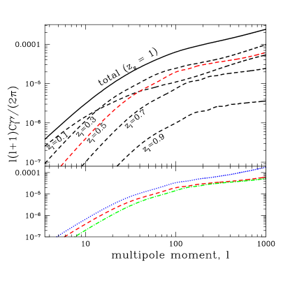
Figure 1: Dependence of the $z=1$ shear auto power spectrum on $g(z)$ and $r(z)$. There are $n-1$ more auto power spectra and $n(n-1)/2$ cross power spectra not shown here. The solid line is the shear power spectrum for sources at $z=1$. The dashed lines show the contributions to this shear power spectrum from lens slices of width $\Delta z=0.2$ centered at $z=0.1,0.3,0.5,0.7$ and 0.9. Their sum gives the solid line. The lower panel shows the $z=0.5$ contribution again (dashed line), how it would look with an increase in $g(z=0.5)$ (dotted line) and how it would look with an increase in $r(z=0.5)$ (dot-dashed line).

Reconstructing $r(z)$ and $g(z)$: Quantitative. Our procedure is a modification of that in song05 where simultaneous reconstruction of distances and growth factors from cosmic shear data was first considered.

We parameterize $r(z)$ by its values specified at discrete redshift values $z_{i}=0.4i$ for $i=1$ to 8. In addition we set $r(z_{*})=r_{s}/\theta_{s}$ where $z_{*}\simeq 1089$ is the redshift of last-scattering. The sound horizon at last-scattering, $r_{s}$, depends on $\rho_{m}$ and $\rho_{b}$. These and the angular size of the sound horizon, $\theta_{s}$, are constrained by CMB observations. The values of $r$ at all other points of $z$ are found by linear interpolation. The $\Delta^{2}(k,z(r))$ factor in Eq. 1 is evaluated by inverting $r(z)$ to get $z(r)$.

We assume that the primordial curvature power spectrum, with amplitude at wavenumber $k$ specified at horizon crossing (when $k/a=H$), is a quasi-power law with logarithmically varying spectral index, $n_{S}(k)=n_{S}+\alpha_{S}\ln(k/k_{f})$ where $k_{f}=0.05$Mpc^-1. This is the form of the expected power spectrum from inflation. The power spectrum at fixed time (or redshift) is related to this primordial power spectrum by a scale-dependent transfer function, $T(k)$ and a growth factor, $g(z)$ so that

$$\Delta^{2}_{\rm lin}(k,z)=\frac{2\pi^{2}}{k^{3}}A_{0}(k/k_{f})^{n_{S}(k)-1}g^{2}(z)T^{2}(k)$$ (2)

In general the time and scale-dependence do not factor as written here, but we are interested in sufficiently small scales where the dark energy perturbations can be ignored and in this case all modes grow at the same rate. The ‘lin’ subscript on $\Delta^{2}$ here stands for ‘linear theory’. We take non-linear evolution into account using the prescription of Peacock and Dodds peacock96 .

We parameterize $g^{2}(z)/a^{2}(z)$ by its value at the eight discrete redshifts used for parameterizing $r(z)$, plus its value at $z=0$. We assume $g(z_{*})=a(z_{*})$, as is the case in the matter-dominated era, and calculate $g^{2}(z)/a^{2}(z)$ at non-grid values of $z$ by linear interpolation.

The transfer function above depends on the matter content. In addition to $A_{0}$, $n_{S}$ and $\alpha_{S}$, the shear power spectra are also therefore affected by $\rho_{m}$, $\rho_{b}$ and the energy density of the cosmological neutrino background. To control these contributions we assume we have a measurement of the CMB temperature and polarization power spectra as expected from Planck. Since these CMB power spectra are also affected by the redshift of reionization, $z_{ri}$, and the primordial fraction of baryonic mass in ⁴He, $Y_{p}$, we include these parameters as well. Our parameter set is thus $\theta_{s}$, $A_{0}$, $n_{S}$, $\alpha_{S}$, $\rho_{m}$, $\rho_{b}$, $z_{ri}$, $m_{\nu}$, $Y_{P}$), eight $r(z)$ parameters and nine $g^{2}(z)/a^{2}(z)$ parameters.

To forecast errors, we Taylor expand to first order the dependence of the shear power spectra on these parameters about our fiducial model. The expected covariance matrix for the errors in the estimated parameters can then be calculated via, e.g., Eq. 21 of song04 .

Acceleration Without Dark Energy. As an example of acceleration without dark energy we turn to the ‘self-inflating’ branch of the DGP model dvali00 . In this model our 3+1-dimensional world (or ‘brane’) is embedded in a 4+1-dimensional space. The Friedmann equation on the brane becomes

$$H^{2}-H/r_{c}=\frac{8\pi G}{3}\rho_{m}$$ (3)

and thus $H$ tends to a constant ($1/r_{c}$) as the Universe expands, just as it would with the usual Friedmann equation in the presence of a cosmological constant.

The extra dimension also leads to a modification of the Poisson term on scales between a smaller scale that is perhaps about 1 Mpc and a large scale, $r_{c}$. Song song05 shows this to be

$$k^{2}/a^{2}\Phi=\frac{3}{2}H^{2}\left[\frac{1-H^{-1}/r_{c}}{1-H^{-1}/(2r_{c})}\right]\delta$$ (4)

where $\delta\equiv\delta\rho_{m}/\bar{\rho}_{m}$ . Growth is suppressed in DGP gravity relative to dark matter only Einstein gravity by the factor in square brackets. However, dark energy also suppresses growth by $\bar{\rho}_{m}/\bar{\rho}_{\rm tot}$, which, for Einstein gravity, replaces the factor in square brackets. In the following we set $r_{c}=1.27/H_{0}$song05 . For non-linear growth we apply the Peacock and Dodds prescription, as we do for Einstein gravity, although consequences of the DGP model for non-linear growth are at the moment unclear.

Quantitative Forecasts for a Fiducial Survey. We take the fiducial survey to be the “2$\pi$” deep wide survey of 20,000 square degrees in six wavelength bands from 0.4-1.1 $\mu$m to be undertaken by the Large Synoptic Survey Telescope ($LSST$). Several hundred sky-noise limited exposures in each optical band will be obtained for each 10 square degree sky patch over a period of ten years. The shapes of galaxies out to a redshift of 3 (integrated galaxy density of 50 per square arcminute) will be measured at a precision far exceeding the 0.15 intrinsic random shear of an individual source galaxy. These galaxy redshifts will be estimated from fits of the 6-band fluxes to spectral templates for galaxies vs type and redshift, a technique called photometric redshift estimation.

This survey will yield the shear and redshift of 3 billion source galaxies over a redshift range of 0.2 - 3. Based on experiments with the active optics 8m Subaru telescope, systematic shear error will be kept below 0.0001 on all angular scales considered here.

Here we model the noise in the resulting shear maps as in song04 . Our analysis does not include effects of redshift errors. For systematic errors in distance determinations to be less than 1%, it is sufficient to require $\Delta z/z<0.01$ (since $r$ varies slower than linearly with $z$) where $\Delta z$ is the error in the mean redshift of a given redshift bin. Simulations based on current surveys indicate that this level of control is achievable at $z>0.1$ connoly05 .

Calculating $C_{l}^{ij}$ sufficiently accurately at small scales is difficult zhan04 ; white04 . We conservatively discarded data at $l>1000$. We have not modeled fluctuations in the dark energy, which can be important on large scales, and therefore discard data with $l<40$ as in song04 .

Results. Our results are presented in Fig. 2. To simulate reconstructed $r(z)$ and $g(z)$ we add a realization of the errors, drawn from a zero mean multivariate Gaussian with our forecasted covariance matrix, to the fiducial values for $r(z)$ and $g(z)$. The error bars are the square root of the diagonal elements of this covariance matrix.

Figure 2: Reconstructed distances (left panels), and growth factors (right panels). The lower left panel shows the fractional residual distances, $[r(z)-r_{\rm fid}(z)]/r_{\rm fid}(z)$, where $r(z)$ are the reconstructed distances and $r_{\rm fid}(z)$ are the distances in the fiducial DGP model. The lower right panel shows the residual growth factor, $g(z)-g_{\rm fid}(z)$. The curves in the right panels are $g_{\rm fid}(z)$ (solid) and $g(z)$ for the Einstein gravity model (dashed) with the same $H(z)$ and $\rho_{m}$ as the DGP model. Although these two models have the same $r(z)$ they are distinguishable by their significantly different growth factors.

Distances are reconstructed with $\sim$ 2% errors, even out to $z=3.2$. The distance errors are highly correlated; certain linear combinations will have even smaller errors. The growth factors have 3% to 4% errors at $z\leq 1.2$ and then grow steadily with $z$. The tightness of the constraint at $z=3.2$ is an artifact of our parameterization. It is due to the $g^{2}(3.2)/a^{2}(3.2)$ parameter influencing $g(z)$ all the way out to $z_{*}$ because of our interpolation scheme.

One can distinguish dark energy from the DGP model even if the dark energy density evolution is adjusted to match $r(z)$ for the DGP model. As mentioned above, these two scenarios will make different predictions for $g(z)$. In the right panels the $g(z)$ curves for the fiducial DGP model and for the dark energy model with identical $H(z)$ are shown. Their difference in $\chi^{2}$ values is 221, corresponding to almost $15\sigma$.

As a test of our calculations, we used our covariance matrix for $r(z)$ and $g(z)$ to calculate constraints on $w$, assuming a dark energy model with constant $w\equiv P/\rho$. The results agree with a more direct calculation of the expected error in $w$ that bypasses the $g$ and $r$ parameterization. The constraint on $w$ is almost entirely due to $r$ constraints rather than $g$ constraints. The roles of geometry and growth are also discussed in zhang03 ; simpson04 .

We note that these measurements of distances into the matter-dominated era, combined with Planck’s CMB observations can be used to achieve $\sigma((\Omega_{\rm tot}-1)h^{2})\sim 10^{-2}$ knox05a , greatly improving the precision with which this robust prediction of inflation can be tested. Allowing for non-zero curvature will mean just one more parameter to fit in our analysis and so will not qualitatively degrade our eight distance determinations.

Discussion and Conclusions. The statistical errors in our fiducial survey are small enough to allow very precise reconstructions of distance and growth as a function of redshift. We have argued that redshift errors will not qualitatively affect our results.

To investigate the impact of shear calibration errors, we parameterized the observed $C_{l}^{ij}$ as $f_{i}f_{j}$ times the true $C_{l}^{ij}$ and extended our parameter set to include one gain parameter, $f_{i}$, for each source redshift bin, $i$. With a 1% prior determination of all the calibration parameters, we find that the distance errors increase by less than 25%, growth errors by less than 35% and $\Delta\chi^{2}$ decreases from 221 to 137. We expect to be able to determine the calibration to even better than 1% from comparison of ground-based data with high-resolution space-based images over a small fraction of the total survey area.

The imaging data from which shear maps are derived can also be used to infer galaxy power spectra. The large-scale feature from matter-radiation equality used here and the baryonic oscillations at smaller scales can also be used to infer distances cooray01 ; seo03 .

The distance-redshift and growth-redshift relations provide two observational windows on the physics of acceleration. While we have illustrated the utility of a second window with a specific example, the extra information may prove crucial to the unraveling of the mystery of acceleration in ways we have not yet imagined.

- (1) A. G. Riess et al., Astron. J.116, 1009 (1998).
- (2) S. Perlmutter et al., Astrophys. J. 517, 565 (1999).
- (3) M. Kaplinghat and M. Turner, Astrophys. J. Lett.569, L19 (2002).
- (4) S. D. M. White, J. F. Navarro, A. E. Evrard, and C. S. Frenk, Nature (London)366, 429 (1993).
- (5) S. Dodelson and L. Knox, Physical Review Letters 84, 3523 (2000).
- (6) D. N. Spergel et al., Astrophys. J. Supp.148, 175 (2003).
- (7) U. J. Leverrier, Mon.Not.Roy.As.Soc.20, 303 (1860).
- (8) C. Csáki, N. Kaloper, and J. Terning, Physical Review Letters 88, 161302 (2002).
- (9) J. Miralda-Escude, Astrophys. J. 380, 1 (1991).
- (10) M. Bartelmann and P. Schneider, Physics Reports340, 291 (2001).
- (11) W. Hu, Astrophys. J. Lett.522, L21 (1999).
- (12) A. Cooray, W. Hu, D. Huterer, and M. Joffre, Astrophys. J. Lett.557, L7 (2001).
- (13) Y.-S. Song, Phys. Rev. D71, 024026 (2005).
- (14) J. A. Peacock and S. J. Dodds, Mon.Not.Roy.As.Soc.280, L19 (1996).
- (15) Y. Song and L. Knox, Phys. Rev. D70, 063510 (2004).
- (16) G. Dvali, G. Gabadadze, and M. Porrati, Physics Letters B 485, 208 (2000).
- (17) A. Connoly et al., in preparation (2005).
- (18) H. Zhan and L. Knox, Astrophys. J. Lett.616, L75 (2004).
- (19) M. White, Astroparticle Physics 22, 211 (2004).
- (20) J. Zhang, L. Hui, and A. Stebbins, ArXiv Astrophysics e-prints (2003).
- (21) F. Simpson and S. Bridle, ArXiv Astrophysics e-prints (2004).
- (22) L. Knox, ArXiv Astrophysics e-prints (2005).
- (23) H. Seo and D. J. Eisenstein, Astrophys. J. 598, 720 (2003).
- (24) A. Nicolis and R. Rattazzi, Journal of High Energy Physics 6, 59 (2004).