• Probing the Origins of Voids in the Distribution of Galaxies

  Louise M. Ord ^A,B,E, Martin Kunz ^B,C, Hugues Mathis ^D, and Joseph Silk ^{D
  A} Department of Astrophysics & Optics, School of Physics, University of New South Wales, Sydney, NSW 2052, Australia
  ^B Astronomy Centre, University of Sussex, Brighton BN1 9QJ, UK
  ^C Theoretical Physics, University of Geneva, 1211 Geneva 4, Switzerland
  ^D Astrophysics, University of Oxford, Denys Wilkinson Building, Keble Road, Oxford OX1 3RH, UK
  ^E Email: louise@phys.unsw.edu.au

  Abstract: If the voids that we see today in the distribution of galaxies existed at recombination, they will leave an imprint on the cosmic microwave background (CMB). On the other hand, if these voids formed much later, their effect on the CMB will be negligible and will not be observed with the current generation of experiments. In this paper presented at the 2004 Annual Scientific Meeting of the Astronomical Society of Australia, we discuss our ongoing investigations into voids of primordial origin. We show that if voids in the cold dark matter distribution existed at the epoch of decoupling, they could contribute significantly to the apparent rise in CMB power on small scales detected by the Cosmic Background Imager (CBI) Deep Field. Here we present our improved method for predicting the effects of primordial voids on the CMB in which we treat a void as an external source in the cold dark matter (CDM) distribution employing a Boltzmann solver. Our improved predictions include the effects of a cosmological constant ($\Lambda$) and acoustic oscillations generated by voids at early times. We find that models with relatively large voids on the last scattering surface predict too much CMB power in an Einstein–de Sitter background cosmology but could be consistent with the current CMB observations in a $\Lambda$CDM universe.
  Keywords: cosmology: theory — cosmic microwave background — large-scale structure of the universe

1 Introduction

Analyses of surveys such as the 2-degree Field Galaxy Redshift Survey and the Sloan Digital Sky Survey indicate large volumes of relatively empty space, or voids, in the distribution of galaxies (e.g. Hoyle & Vogeley, 2002, 2004). In the standard hierarchical model of structure formation, gravitational clustering is responsible for emptying these voids of mass and galaxies (Peebles, 1989). However, standard cold dark matter (CDM) simulations predict significant clumps of substructure within voids that that should be capable of developing into observable bound objects, such as dwarf galaxies, that are not apparent in the surveys (Dekel & Silk, 1986; Hoffman et al., 1992; Shandarin et al., 2004). Peebles, (2001) gives an in-depth discussion of the contradictions of this prediction with observation. He believes that the inability of the CDM models to produce the observed voids constitutes a true crisis for these models.

It has been argued that the apparent suppression of void object formation may be addressed when more sophisticated models for the complex effects of baryons on galaxy formation are developed (e.g. van den Bosh et al., 2000). Others believe that alternatives to CDM, such as warm dark matter (WDM) (Hogan & Dalcanton, 2000; Sommer-Larsen & Dolgov, 2001) or self-interacting dark matter (Spergel & Steinhardt, 2000), may provide a solution. The higher temperature of WDM particles causes them to move faster than particles of CDM. This motion might enable WDM particles to resist congregating to form observable galaxies within voids. However, Barkana et al., (2001) note that the material’s resistance to clumping might delay the epoch of quasar formation and the model is ruled out if reionisation occurred before $z\sim 10$ as indicated by the recent WMAP cosmic microwave background (CMB) data (Spergel et al., 2003).

Self-interacting dark matter may explain the relative dearth of dwarf galaxies. If there were interparticle collisions, the halo of dark matter surrounding a large galaxy would interact with the halos of nearby dwarf galaxies, stripping the dwarves of their gas and stars more rapidly than in the standard CDM theory. However, Chandra X-ray Observatory data indicates that the density of the dark matter is greater the closer it is to the center of the cluster (Arabadjis et al., 2002), in contradiction with the simplest self-interacting dark matter models which predict particle collisions to occur most frequently in more populated regions and act to spread out galactic cores and reduce their density.

The standard CDM model of structure formation remains extremely successful at matching the observations on large scales such as the properties of galaxy clusters, the statistics of the Lyman-$\alpha$ forest and the temperature anisotropy of the CMB. However, the lack of observable dwarf galaxies within voids as predicted by the simulations can not be overlooked. Additionally, recent deep field observations from the Cosmic Background Imager (CBI) Mason et al., (2003) show excess power in the CMB over the standard model on small angular scales, $\ell>2000$.

It may be possible to explain both these observations by postulating the presence of a network of voids originating from primordial bubbles of true vacuum that nucleated during inflation (La, 1991; Liddle & Wands, 1991). In this scenario, the first bubbles to nucleate are stretched by the remaining inflation to cosmological scales. The largest voids may have had insufficient time to thermalise before decoupling and may persist to the present day. Such primordial voids are predicted to produce a measurable contribution to the CMB on small-scales (see Griffiths et al., (2003) and references therein). If voids in the matter distribution were present prior to the onset of gravitational collapse, the formation of bound objects within voids would be suppressed.

In this paper, we discuss the results of Griffiths et al., (2003) in which we develop a general method to approximate the void contribution to the CMB that allows the creation of maps and enables us to consider an arbitrary distribution of void sizes. We show that if the voids that we see in galaxy surveys today existed at the epoch of decoupling, they could contribute significant additional power to the CMB angular power spectrum between $2000<\ell<3000$. Further to Griffiths et al., (2003), we show how we improve our predictions. We include the effects of the cosmological constant as well as oscillations in the matter-radiation fluid that may be generated by primordial voids on scales up to the sound horizon (Baccigalupi & Perrotta, 2000) and present our method for constraining the parameters of this inflationary model of void production.

2 First Approximation

2.1 Void parameters

In Griffiths et al., (2003) we model the voids seen today as spherical underdensities of $\delta\rho/\rho=-1$. As a primordial void bubble nucleates and is stretched by inflation it will sweep up the surrounding energy density to form a thin boundary wall. At the end of the inflationary epoch, any voids that persist will be fully compensated. This means that the overall cosmology is that of the background universe, since a compensated void does not distort space-time outside of itself. This is an extremely important property, as it allows us to place many voids into a universe without the worry that they might influence each other. As a first approximation we take the background universe to be an Einstein–de Sitter (EdS) cosmology. Maeda & Sato, (1983) and Bertschinger, (1995) use conservation of momentum and energy respectively to show that compensated voids in an EdS background cosmology will increase in radius $r_{v}$ between the onset of the gravitational collapse of matter at equality and the present day such that

$$r_{v}(\eta)\propto\eta^{\beta}\,,$$ (1)

with $\beta\approx 0.39$ and where $\eta$ is conformal time.

Motivated by the extended inflationary scenario (La & Steinhardt, 1989, see Kolb 1991 for a review), we assume a power-law distribution of bubble sizes greater than a given radius $r$ of the form,

$$N_{B}(>r)\propto r^{-\alpha}.$$ (2)

Typically, extended inflation is implemented within the framework of a Jordan-Brans-Dicke theory (Brans & Dicke, 1961). In this case, the exponent $\alpha$ is directly related to the gravitational coupling $\omega$ of the scalar field that drives inflation,

$$\alpha=3+\frac{4}{\omega+1/2}.$$ (3)

Values of $\omega>3500$ are required by solar system experiments (Will 2001). We take the limit of large $\omega$, leading to a spectrum of void sizes with $\alpha=3$.

Liddle & Wands, (1991) show that a distribution of void sizes that predicts the existence of arbitrarily large inflationary voids will cause significant effects on the CMB that contradict observations. We assume that the mechanism creating the voids imposes an upper cut-off on the size distribution. A possible mechanism for this cut-off could be that the tunneling probability of inflationary bubbles is modulated through the coupling to another field.

As well as avoiding the well known problems associated with arbitrarily large voids existing at the epoch of decoupling, this assumption allows us to match the observed upper limit on void sizes from the galaxy redshift surveys. Since the results of void finder algorithms in the literature include those obtained from incomplete galaxy surveys, we choose to take the average maximum void size that is found, $r_{\rm max}=25$ Mpc$/h$ (e.g. Hoyle & Vogeley, 2002, 2004). An analysis is also in progress in which this parameter is kept free so that it may be constrained by the observations. The minimal present void size is also chosen to agree with redshift surveys, $r_{\rm min}=10$ Mpc$/h$.

We normalise the distribution by requiring that the total number of voids satisfies the observed fraction of the universe filled with voids today, $F_{v}$. Redshift surveys indicate that approximately 40% of the fractional volume of the universe is in the form of voids of underdensity $\delta\rho/\rho<-0.9$ (e.g. Hoyle & Vogeley, 2002, 2004), ie. $F_{v}\approx 0.4$. The positions of the voids are then assigned randomly, making sure that they do not overlap. In order to speed up this process, we consider only a $10^{\circ}$ cone. This limits our analysis to $\ell>100$, which is satisfactory for our purpose since the main contribution from voids is on much smaller scales.

2.2 Stepping through the void network

Refer to Griffiths et al., (2003) for a more detailed description of our methodology. We ray trace photon paths from us to the last scattering surface (LSS) for the 10^∘ cone in steps of 1’. Each void in the present day distribution that is intersected by the photon path is evolved back in time according to equation (1) to determine whether the photon encounters the void.

If a photon intersects a void between us and the LSS, we compute the Rees–Sciama (RS) (1968) effect due to the deviation in the redshift of the photon as it passes through the expanding void and the lensing effect due to the deviation in its path. If a photon intersects a void on the LSS, we calculate the Sachs–Wolfe (SW) (1967) effect due to the photon originating from within the underdensity. We take into account the finite thickness of the LSS, which suppresses the SW effect for small voids, by averaging the contribution from a number of photons originating from a LSS of mean redshift 1100 and standard deviation in redshift 80. We also calculate the partial RS effect that arises due to the expansion of the void on the LSS as the photon leaves it.

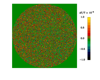
Figure 1: The map of the temperature fluctuations on the surface of last scattering from the fiducial EdS void model considered. The parameters of this model are given by $\alpha=3$, $r_{\rm max}=25$ Mpc$/h$ and $F_{v}=0.4$.

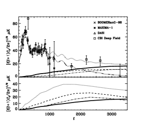
Figure 2: Top: The CMB anisotropies produced by the fiducial EdS void model (solid line) compared to the primary $\Lambda$CDM CMB anisotropies (dashed-triple-dotted). Also plotted are the sum of primary and void contributions (dotted) as well as the fluctuations induced purely by voids on the last scattering surface (dashed) and by those between last scattering and today (dashed-dotted). We show the “standard” cosmological concordance model: of course a combined analysis of primary and void–induced fluctuations would select a different cosmology for the primary contribution. Bottom: Example models depicting a range of void contributions to the CMB fluctuations. The models plotted are $\alpha=3$, $r_{\rm max}=25$ Mpc$/h$ and $F_{v}=0.4$ (solid line), $\alpha=3$, $r_{\rm max}=40$ Mpc$/h$ and $F_{v}=0.4$ (dotted), $\alpha=3$, $r_{\rm max}=40$ Mpc$/h$ and $F_{v}=0.2$ (dashed) and $\alpha=6$, $r_{\rm max}=40$ Mpc$/h$ and $F_{v}=0.4$ (dashed-dotted).

Once the photon has reached the last scattering surface, we know the variation of its temperature as well as its position on the LSS and can create a temperature map (figure 1). We then use a flat sky approximation (White et al., 1999; da Silva, 2002) to obtain the $C_{\ell}$ spectrum of the anisotropies (see figure 2). We point out that primordial void parameters are still poorly constrained by both observation and theory. The bottom panel of figure 2 shows a few further example models.

For a power-law size distribution (as motivated by the inflationary scenario), large voids become rarer as $\alpha$ is increased. Therefore, since void analyses of redshift surveys only sample a fraction of the volume of the universe, there may exist voids of larger $r_{\rm max}$ than currently observed. Models with high $r_{\rm max}$ voids in an EdS background cosmology tend to predict too much power on scales $\ell\approx 1000$. However, if we take inflationary models with $\alpha>6$, as motivated by eg. Occionero & Amendola, (1994), then the peak moves to larger $\ell$ and the total power drops. The filling fraction mainly adjusts the overall power.

3 Improved Prediction

3.1 Void Evolution in a $\Lambda$CDM background cosmology

The addition of a cosmological constant ($\Lambda$) to the cosmology is expected to slow down the conformal evolution of the voids at late times. We test this hypothesis by simulating the comoving evolution of a single void of radius $25$ Mpc$/h$ starting at $z=1000$ in a $(100$ Mpc$/h)^{3}$ box containing $64^{3}$ particles. We find that the void size evolution in a $\Lambda$CDM background deviates from that of the EdS scaling solution at late times as expected. However, the final radius is underestimated by less than 2% (see figure 3). The EdS void scaling relationship given by equation (1) with $\beta=0.39$ is therefore a good approximation for a void in a $\Lambda$CDM background.

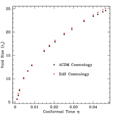
Figure 3: The simulated size evolution for a 25 Mpc$/h$ void in a $\Lambda$CDM background cosmology (triangles) compared with the scaling relationship (equation 1 with $\beta=0.39$) for an EdS background (crosses). The two evolutions deviate by less than 2% at $\eta=0.046$, the current age of the universe.

Since a $\Lambda$CDM universe evolves for substantially longer, we would expect the voids that we see today to appear smaller on the last scattering surface for this cosmology than in our first approximation EdS background. We would therefore predict that voids in a $\Lambda$CDM universe will have a more suppressed effect on the CMB than we have first approximated. This can be modelled by taking the horizon size of our cone of voids to be that of a $\Lambda$CDM cosmology. Figure 4 compares the predicted power from a uniform distribution of equally sized voids in EdS and $\Lambda$CDM background cosmologies. The overall contribution to the CMB from the voids is suppressed as expected and the peak is moved to smaller angular scales since the voids now appear smaller on the last scattering surface.

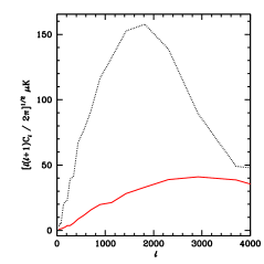
Figure 4: The predicted CMB power from a uniform distribution of equally sized voids in EdS (dotted) and $\Lambda$CDM (solid) background universes. The voids have a size of 40 Mpc$/h$ and a filling fraction of $40$ %. The void contribution is computed by ray tracing a void network. The effect of $\Lambda$ is to suppress the effect of the voids and move the peak in the power spectrum to smaller angular scales since they will appear smaller on the last scattering surface.

3.2 Modelling acoustic oscillations

So far we have studied voids which do not interact with their surroundings. Specifically, they do not perturb the matter-radiation fluid themselves. While this is a reasonable approximation for the RS effect after recombination, it has been pointed out (Baccigalupi & Perrotta, 2000) that this is not true before last scattering. A void could therefore set up oscillations in the matter-radiation fluid on scales up to the sound horizon, which might be clearly visible in the power spectrum.

The standard way to include the full behaviour of matter and radiation perturbations is to solve the Boltzmann equation numerically. But it is not possible to model a void self-consistently inside the Boltzmann solver. The dark matter density contrast inside the void becomes very large (approaching $-1$ at late times) and is clearly non-perturbative. A similar problem was encountered a few years ago while investigating topological defects (see Durrer et al., (2002) and references therein). The solution in this case was to model the defects as external sources. This can be done for the voids as well. Any back reaction from the perturbation on the voids should only be second order so can be neglected. Furthermore, the connection between the external source (the voids) and the matter-radiation fluid is via the metric perturbations $\Phi$ and $\Psi$ and, since they are small during the times of interest, they can hence be handled within a perturbative framework.

As opposed to defects, which are entirely external sources, the voids represent a perturbation of the dark matter. By construction, the dark matter is in a stable configuration and does not perturb itself. It is therefore influenced by the presence of the void. Also, since there is no dark matter inside the void, there can be no flow outwards. We have chosen to model these effects by making the approximation that the dark matter is completely decoupled from the rest of the universe. Therefore, the cold dark matter acts only as an external seed where the perturbations are concerned (of course it is taken into account for the background quantities).

We assume that perturbations driving away from the void configuration are only due to the back-reaction from the induced perturbations in the other fluids. As these are second order effects, we can neglect them. We could take them into account by coupling the dark matter to the fluid perturbations alone. However, as expected, the effect on the resulting power spectrum is minor, around 1% for the scales of interest which is comparable to the accuracy of the Boltzmann codes. We prefer to use first order perturbation theory consistently and turn the dark matter perturbations off completely.

We assume that the photons and baryons have flown relativistically back into the void, while the cold dark matter remained frozen in the wall. We therefore choose a density contrast

$$\delta=-\frac{\rho_{c}}{\rho_{\gamma}+\rho_{\nu}+\rho_{b}+\rho_{c}}=-\frac{\Omega_{c}}{\Omega_{\rm rel}/a+\Omega_{c}+\Omega_{b}}\,.$$ (4)

In the phenomenological model investigated here, the voids emerge slowly from the isotropic background of relativistic particles during inflation. Therefore, equation 4 also describes the void density contrast at high redshifts. A more violent formation history can lead to stronger acoustic waves and change our results.

Following the formalism of Kunz & Durrer, (1997), Durrer & Sakellariadou, (1997) and Durrer et al., (1999), the source is found to be

$$\Phi(\eta,{\mathbf{k}}) = -\frac{4\pi}{\sqrt{\eta_{0}^{3}}}\left(\frac{a^{\prime}}{a}\right)^{2}\delta\,f(k,r_{v}(\eta))$$ (5)

$$f(k,r) = \frac{\left(3-(kr)^{2}\right)\sin(kr)-3kr\cos(kr)}{k^{5}}\,.$$ (6)

We insert this source into a modified version of CMBEasy (Doran, 2003). We then write out a snapshot of the fluids at the time of last scattering and Fourier transform them back.

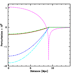
Figure 5: The behaviour of the perturbations in real space at last scattering (LS) from a single void. The void, which has a radius of 40 Mpc today, has a comoving size of 9 Mpc at LS. The black solid curve is the input perturbation $\Phi_{S}(x,\eta_{LS})/2$, while the red dotted curve is the total metric perturbation $\Phi$/2. The blue small dashed curve shows $-2\Psi=2\Phi$. The cyan large dashed curve is the temperature perturbation from the photons, $D_{g}/4$. The baryon velocity is shown as the magenta dot-dashed curve. The green small dashed-large dashed curve is $D_{g}/4-2\Phi$, which is very similar to $\Phi_{S}/2$.

Figure 6 shows a close up of the perturbations around the sound horizon. These are due to oscillations set up during the formation of the void and are therefore strongly dependent on the formation history of the void. With our form of $\delta(\eta)$, given by equation (4), we see that the amplitude of the sound waves is only about 1% of the amplitude of the temperature perturbations inside the void. For smaller voids, the relative amplitude will be even less. This seems quite unimportant, indeed, the oscillations are not even visible in figure 5. However, the void itself covers a surface of only about $9^{2}\pi({\rm Mpc}/h)^{2}$ on the LSS, the sound horizon in our flat matter dominated universe of the example case is at $111{\rm Mpc}/h$ and the sound waves extend out to about $100{\rm Mpc}/h$, ten times further than the size of the void. Therefore, the total power in the fluctuations is about $100$ times larger than expected from their amplitude and is comparable to the the power from the void predicted by our first approximation method. Indeed, we see oscillations appear on large angular scales in the angular power spectrum (see figure 7).

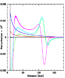
Figure 6: A “zoom” onto the sound waves generated by the void. Notice that the x axis now extends beyond the sound horizon (at about $111$ Mpc) and that the y axis has been magnified by roughly a factor 1000 compared to fig. 5. The lines are the same as in that figure.

3.3 Correlation function approach

In order to calculate the angular power spectrum of the CMB, we can again use a technique developed for studying topological defects, namely the use of unequal time correlators Turok, (1996). The modified Boltzmann equation described above is just a system of linear equations,

$${\mathcal{D}}X={\mathcal{S}}.$$ (7)

Here ${\mathcal{D}}$ is a time dependent linear differential operator, $X$ is the vector of perturbation variables and ${\mathcal{S}}$ the source term. For one single void, the source is deterministic. But in general we are interested in a void network with a random distribution of both the position and sizes of the voids. In this case the source becomes a random variable.

For any given initial conditions we can formally solve the Boltzmann equation by means of a Greens function ${\mathcal{G}}$,

$$X_{j}(t_{0},{\mathbf{k}})=\int_{t_{\rm in}}^{t_{0}}dt\,{\mathcal{G}}_{j}(t_{0},t,{\mathbf{k}})S(t,{\mathbf{k}})\,.$$ (8)

The power spectrum is then a quadratic expectation value of the form

$$\begin{array}[]{l}C_{\ell}\sim\left\langle X_{j}(t_{0},{\mathbf{k}})X_{l}^{*}(t_{0},{\mathbf{k}})\right\rangle=\\ \int_{t_{\rm in}}^{t_{0}}dt{\mathcal{G}}_{j}(t_{0},t,{\mathbf{k}})\int_{t_{\rm in}}^{t_{0}}dt^{\prime}{\mathcal{G}}_{l}(t_{0},t^{\prime},{\mathbf{k}})\left\langle{\mathcal{S}}(t,{\mathbf{k}}){\mathcal{S}}^{*}(t^{\prime},{\mathbf{k}})\right\rangle\,,\end{array}$$ (9)

and we need to study the unequal time correlation function (UTC) of the source in more detail,

$$\left\langle\Phi(t,{\mathbf{k}})\Phi^{*}(t^{\prime},{\mathbf{k}})\right\rangle.$$ (10)

As the $\Phi$ of the different voids don’t overlap in real space, we can just add them up to create the total $\Phi$ of the void network,

$$\Phi_{\rm tot} = \sum_{j}\Phi_{j}$$ (11)

$$= \sum_{j}\Phi^{(R_{j})}({\mathbf{x}}-{\mathbf{c}}_{j}).$$ (12)

The sum runs over all voids, $R_{j}$ is today’s radius of void $j$ and ${\mathbf{c}}_{j}$ is the centre of void $j$. Going into Fourier space we find

$$\Phi(t,{\mathbf{k}}) = \int d{\mathbf{x}}\Phi(t,{\mathbf{x}})e^{i{\mathbf{k}}{\mathbf{x}}}$$ (13)

$$= \sum_{j}\int d{\mathbf{x}}\Phi^{(R_{j})}(t,{\mathbf{x}}-{\mathbf{c}}_{j})e^{i{\mathbf{k}}{\mathbf{x}}}$$ (14)

$$= \sum_{j}\Phi^{(R_{j})}(t,{\mathbf{k}})e^{i{\mathbf{k}}{\mathbf{c}}_{j}}\,.$$ (15)

The function $\Phi^{(R_{j})}(t,{\mathbf{k}})$ is just the Fourier space source for a single void at the origin with radius $R_{j}$ at time $t$ as given in equation (6). The different spatial positions of the voids are now encoded only in an additional phase factor. The UTC required for computing the power spectrum is

$$\sum_{j,l}\Phi^{(R_{j})}(t,{\mathbf{k}})\Phi^{(R_{l})}(t^{\prime},{\mathbf{k}})e^{i{\mathbf{k}}({\mathbf{c}}_{j}-{\mathbf{c}}_{l})}.$$ (16)

Let us first discuss the special case of equal-sized voids, $R_{j}\equiv R\,\,\forall j$. In this case we can move the metric perturbation $\Phi$ outside the sum and the UTC can be separated into two parts,

$$\left\langle{\mathcal{S}}(t,{\mathbf{k}}){\mathcal{S}}^{*}(t^{\prime},{\mathbf{k}})\right\rangle.=\Phi^{(R)}(t,{\mathbf{k}})f({\mathbf{k}})\,\Phi^{(R)*}(t^{\prime},{\mathbf{k}})f({\mathbf{k}})$$ (17)

where the $\Phi^{(R)}$ are again the single void metric perturbations of equation (6) and

$$f({\mathbf{k}})=\sqrt{\sum_{j,l}e^{i{\mathbf{k}}({\mathbf{c}}_{j}-{\mathbf{c}}_{l})}}$$ (18)

The contribution to $f$ can be naturally separated into two different parts, namely the contribution with $i=j$ which amounts to $\sqrt{N_{\rm void}}$, the square root of the number of voids in the universe, and the contribution with $i\neq j$ which is a superposition of oscillations with different frequencies, given by the distance between the voids. These oscillations will in general tend to cancel out so that we are left with $f({\mathbf{k}})\approx\sqrt{N_{\rm void}}$.

The fact that the UTC separates into two parts is crucial, since it permits us to integrate independently over $t$ and $t^{\prime}$ in equation (9). Each integral amounts to the same as solving the Boltzmann equation with the source

$${\mathcal{S}}(t,{\mathbf{k}})=\Phi^{(R)}(t,{\mathbf{k}})f({\mathbf{k}})$$ (19)

and since they are the same, the angular power spectrum is just the one computed with this source.

By setting $f({\mathbf{k}})\approx\sqrt{N_{\rm void}}$ as discussed above, and writing $C^{(R)}_{\ell}$ for the power spectrum which we get with a single void as a source, we find

$$C_{\ell}\approx N_{\rm void}C^{(R)}_{\ell}$$ (20)

and not $C_{\ell}\approx N^{2}_{\rm void}C^{(R)}_{\ell}$ as might have been guessed naively, the power spectrum being quadratic in $\delta T/T$.

In the general case of equation 16 we cannot separate the UTC into two parts. But now the oscillations in the $exp\{i{\mathbf{k}}({\mathbf{c}}_{j}-{\mathbf{c}}_{l})\}$ term are being helped to average out by the now incoherent oscillations from the $\Phi^{(R_{j})}$ with different radii (as long as the void radii and the void positions are not correlated). We therefore expect the main contribution to the source to come from $i=j$, leaving us with

$$\sum_{j}\Phi^{(R_{j})}(t,{\mathbf{k}})\Phi^{(R_{j})}(t^{\prime},{\mathbf{k}})$$ (21)

as the source. This is a sum of a source which separates into two equal parts. Again writing $C^{(R)}_{\ell}$ for the single-void power spectrum, we find

$$C_{\ell}=\sum_{j}C^{(R_{j})}_{\ell}.$$ (22)

This can be summed up using an actual realisation of a void distribution. But since we are mainly interested in the average result for the theoretical distribution, we can use this distribution directly. Writing $\rho(R)dR$ for the number of voids with radii between $R$ and $R+dR$ the total power spectrum becomes

$$C_{\ell}=\int dR\rho(R)C^{(R)}_{\ell}.$$ (23)

3.4 Boltzmann imprint of primordial voids on the power spectrum

Figure 7 compares the void $C_{\ell}$ from ray tracing and the Boltzmann approach for a uniform distribution of $40$ Mpc$/h$ sized voids. The overall effect from the first approximation ray tracing method appears to be suppressed using the improved Boltzmann solution. Evidence of acoustic oscillations generated in the photon-baryon fluid can also be seen on large angular scales. The RS effect due to $\Phi_{v}$ alone, using the same approximations in both calculations, is in agreement for both methods as expected.

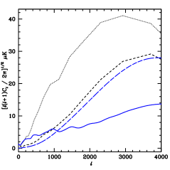
Figure 7: We compare the $C_{\ell}$ from ray tracing and the Boltzmann approach. The dotted curve shows the total $\delta T$ for a $\Lambda$CDM model with voids of a size of $40$ Mpc$/h$ and a filling fraction of $40$ %, computed by ray tracing a void network. The solid curve shows the same but computed with a Boltzmann code. The small and large dashed lines show the RS effect due to $\Phi_{v}$ alone for both methods and with the same approximations, these two curves should coincide.

The suppression that is evident using the Boltzmann solution over the ray tracing approach is due to a number of factors. In the ray tracing method we assume that the density contrast $\delta=-1$ and we take $(a^{\prime}/a)^{2}$ to be $4/\eta^{2}$. Close to radiation domination (ie. at early times, just after last scattering, when we get the biggest effect) both these approximations act to increase the ray tracing result with respect to the more accurate Boltzmann prediction, together by more than a factor of 2. The ray tracing method also neglects the Doppler contribution from the baryon velocity, which suppresses the result further. Finally, the finite thickness of the LSS and Silk damping were not fully taken into account in our first approximation ray tracing method.

The parameter $r_{\rm max}$ is currently fixed using a number of void analyses of surveys, including the 2-degree Field Galaxy Redshift survey (Hoyle & Vogeley, 2004). As discussed in subsection 2.2, these surveys only sample a fraction of the volume of the universe. Therefore, the existence of voids of larger $r_{\rm max}$ than currently observed can not be ruled out. Models with $\alpha=3$ and high $r_{\rm max}$ voids in an EdS background cosmology tend to predict too much power on scales $\ell\approx 1000$. Our results show that this is less of a problem for a $\Lambda$CDM universe. Furthermore, since the Boltzmann solution predicts the CMB power from voids to be lower than implied by the ray tracing estimation, relatively large voids on the last scattering surface may be consistent with the current CMB data, even for void distributions with low values of $\alpha$ (see figure 8).

Figure 8: Top: The CMB anisotropies produced by a $\Lambda$CDM void model (solid line: $\alpha=3$, $r_{\rm max}=55$ Mpc$/h$ and $F_{v}=0.4$) compared to the primary $\Lambda$CDM anisotropies (dotted). Also plotted are the sum of primary and void contributions (dashed). We show the “standard” cosmological concordance model. Again a combined analysis of primary and void–induced fluctuations would select a different cosmology for the primary contribution. Bottom: The large dashed curve shows the fiducial EdS model of figure 2 ($\alpha=3$, $r_{\rm max}=25$ Mpc$/h$ and $F_{v}=0.4$) using our ray tracing method. The same model is shown for our Boltzmann solution with EdS (small dashed) and $\Lambda$CDM (dotted) background universes. The solid bold line is the same $\Lambda$CDM void model for $r_{\rm max}=55$ Mpc$/h$ maximally sized voids as in the panel above.

4 Conclusions

The cosmic microwave background is an excellent tool for probing the distribution of matter from last scattering until today. In the case of voids, the strongest signal stems from objects at very high redshifts, especially from those already present at decoupling. We discuss in this Paper our improved method to investigate the imprint of a distribution of primordial, spherical and compensated voids, which could for example be generated by a phase transition during inflation.

We show that the signature of a power-law distribution of such voids, that is compatible with redshift sureys, contributes additional power on small angular scales. The amount of power generated depends on the parameters that describe the void size distribution as well as the background cosmology. The overall signal predicted by our first approximation ray tracing method is somewhat suppressed using our improved Boltzmann solution. Thus, primordial void formation models that produce relatively large voids on the last-scattering surface may not be ruled out by the current CMB observations.

Experiments such as the CBI are able to directly probe small angular scales and constrain void parameters. We will present a Markov Chain Monte Carlo constraints analysis of a wide range of void models in a future paper. We will further constrain models that are compatible with CMB observations using cluster evolution (Mathis et al., 2004) and also investigate the non-Gaussian signal of void models that are compatible with the observations.

Other sources are also expected to contribute at high $\ell$. Probably the strongest of these is the thermal Sunyaev-Zel’dovich (SZ) effect. Since the thermal SZ effect is strongly frequency–dependent, experiments which work at about 30 GHz (like CBI) will see a stronger signal than those working at higher frequencies (Aghanim et al., 2002). Hence a multi-frequency approach should be able to easily disentangle the contribution of voids from the SZ effect. Unfortunately, it seems to be difficult at present to predict the precise level of the SZ contribution, since different groups are reporting different results (see eg. Springel et al., (2001) for a compilation). Future multi-frequency, high resolution and high signal-to-noise maps should be able to significantly constrain the contribution of primordial voids to the high $\ell$ CMB power spectrum. Additionally, deep galaxy redshift surveys and measurements of the distribution of matter in the Ly-$\alpha$ forest will be able to directly explore the presence of voids in the baryonic matter distribution at low redshifts.

References

- Aghanim et al., (2002) Aghanim, N., Castro, P. G., Melchiorri, A., Silk, J., 2002, Astron. & Astrophys., 393, 381.
- Arabadjis et al., (2002) Arabadjis, J. S., Bautz, M. W., Garmire, G. P., 2002, Astrophys. J., 572, 66.
- Baccigalupi & Perrotta, (2000) Baccigalupi, C., Perrotta, F., 2000, Mon. Not. R. Astron. Soc., 314, 1.
- Barkana et al., (2001) Barkana, R., Haiman, Z., Ostriker, J. P., 2001, Astrophys. J., 558, 482.
- Bertschinger, (1995) Bertschinger, E., 1985, Astrophys. J. Supp., 58, 1.
- Brans & Dicke, (1961) Brans, C., Dicke, C. H., 1961, Phys. Rev., 24, 925.
- da Silva, (2002) da Silva A., 2002, The Sunyaev-Zel’dovich effect: predictions from Hydrodynamical N-Body Simulations, DPhil Thesis, University of Sussex.
- Dekel & Silk, (1986) Dekel, A., Silk, J., 1986, Astrophys. J., 303, 39.
- Doran, (2003) Doran, M., 2003, astro-ph/0302138.
- Durrer & Sakellariadou, (1997) Durrer, R., Sakellariadou, M., 1997, Phys. Rev. D 56, 4480.
- Durrer et al., (1999) Durrer, R., Kunz, M., Melchiorri, A., 1999, Phys. Rev. D, 59, 123005.
- Durrer et al., (2002) Durrer, R., Kunz, M., Melchiorri, A., 2002, Phys. Rept. 364, 1.
- Griffiths et al., (2003) Griffiths, L. M., Kunz, M., Silk, J., 2003, Mon. Not. R. Astron. Soc., 339, 680.
- Hoffman et al., (1992) Hoffman, Y., Silk, J., Wyse, R. F. G., 1992, Astrophys. J. Lett., 388, L13.
- Hogan & Dalcanton, (2000) Hogan, C. J., Dalcanton, J. J., 2000, Phys. Rev. D, 62, 063511.
- Hoyle & Vogeley, (2002) Hoyle, F., Vogeley, M. S., 2002, Astrophys. J., 566, 641.
- Hoyle & Vogeley, (2004) Hoyle, F., Vogeley, M. S., 2004, Astrophys. J., 607, 751.
- Kolb, (1991) Kolb, E. W., 1991, in The Birth and Early Evolution of the Universe, Proceedings of the 1990 Nobel Symposium.
- Kunz & Durrer, (1997) Kunz, M., Durrer, R., 1997, Phys. Rev. D 55, 4516.
- La, (1991) La, D., 1991, Phys. Lett. B, 265, 232.
- La & Steinhardt, (1989) La, D., Steinhardt, P. J., 1989, Phys. Rev. Lett., 62, 376.
- Liddle & Wands, (1991) Liddle, A. R., Wands, D., 1991, Mon. Not. R. Astron. Soc., 253, 637.
- Maeda & Sato, (1983) Maeda, K., Sato, H., 1983, Progr. Theor. Phys., 70, 772.
- Mason et al., (2003) Mason, B. S., et al., 2003, Astrophys. J., 591, 540.
- Mathis et al., (2004) Mathis, H., Silk, J., Griffiths, L. M., Kunz, M., 2004, Mon. Not. R. Ast. Soc., 350, 287.
- Occionero & Amendola, (1994) Occhionero, F., Amendola, L., 1994, Phys. Rev. D, 50, 4846.
- Peebles, (1989) Peebles, P. J. E., 1989, J. R. Astron. Soc. Canada, 83, 363.
- Peebles, (2001) Peebles, P. J. E., 2001, Astrophys. J., 557, 495.
- Rees & Sciama, (1968) Rees, M. J., Sciama, D., 1968, Nature, 217, 511.
- Sachs & Wolfe, (1967) Sachs, R. K., Wolfe, A. M., 1967, Astrophys. J., 147, 73.
- Shandarin et al., (2004) Shandarin, S. F., Sheth, J. V., Sahni, V., 2004, Mon. Not. R. Astron. Soc., 353, 162.
- Sommer-Larsen & Dolgov, (2001) Sommer-Larsen, J., Dolgov, A., 2001, Astrophys. J., 551, 608.
- Spergel & Steinhardt, (2000) Spergel, D. N., Steinhardt, P. J., 2000, Phys. Rev. Lett., 84, 3760.
- Spergel et al., (2003) Spergel, D. N., et al., 2003, Astrophys. J. Supp., 148, 175.
- Springel et al., (2001) Springel, V., White, M., Hernquist, L., 2001, Astrophys. J., 549, 681.
- Turok, (1996) Turok, N., 1996, Phys. Rev. D 54, 3686.
- van den Bosh et al., (2000) van den Bosch, F. C., Robertson, B. E., Dalcanton, J. J., de Blok, W. J. G., 2000, Astronom. J., 119, 1579.
- White et al., (1999) White, M., Carlstrom, J. E., Dragovan, M., Holzapfel, W. L., 1999, Astrophys. J., 514, 12.
- Will, (2001) Will, C. M., 2001, Living Rev. Rel., 4, 4.