Lyman Break Galaxies at $z=4-6$ in cosmological SPH simulations

Abstract

We perform a spectrophotometric analysis of galaxies at redshifts $z=4-6$ in cosmological SPH simulations of a $\Lambda$ cold dark matter ($\Lambda$CDM) universe. Our models include radiative cooling and heating by a uniform UV background, star formation, supernova feedback, and a phenomenological model for galactic winds. Analysing a series of simulations of varying boxsize and particle number allows us to isolate the impact of numerical resolution on our results. Specifically, we determine the luminosity functions in $B$, $V$, $R$, $i^{\prime}$, and $z^{\prime}$ filters, and compare the results with observational surveys of Lyman break galaxies (LBGs) performed with the Subaru telescope and the Hubble Space Telescope. We find that the simulated galaxies have UV colours consistent with observations and fall in the expected region of the colour-colour diagrams used by the Subaru group. The stellar masses of the most massive galaxies in our largest simulation increase their stellar mass from $M_{\star}\sim 10^{11}M_{\odot}$ at $z=6$ to $M_{\star}\sim 10^{11.7}M_{\odot}$ at $z=3$. Assuming a uniform extinction of $E(B-V)=0.15$, we also find reasonable agreement between simulations and observations in the space density of UV bright galaxies at $z=3-6$, down to the magnitude limit of each survey. For the same moderate extinction level of $E(B-V)\sim 0.15$, the simulated luminosity functions match observational data, but have a steep faint-end slope with $\alpha\sim-2.0$. We discuss the implications of the steep faint-end slope found in the simulations. Our results confirm the generic conclusion from earlier numerical studies that UV bright LBGs at $z\geq 3$ are the most massive galaxies with $E(B-V)\sim 0.15$ at each epoch.

1 Introduction

Numerical simulations of galaxy formation evolve a comoving volume of the Universe, starting from an initial state given by the theory of inflation. Such simulations are in principle capable of accurately predicting the properties of galaxies that form from these initial conditions, but limited computer resources impose severe restrictions on the resolution and volume size that can be reached. In general, it is easier to achieve sufficient numerical resolution for high redshift galaxies because the Universe is young and simulations are evolved forward in time from the Big Bang. However, observational surveys are often mainly limited to low redshifts, looking outwards and backwards in time from our vantage point. In recent years, significant advances in both observational and numerical techniques have created an optimal overlap range between the two approaches at intermediate redshifts ($z=2-6$), which is therefore a promising epoch for comparing theoretical predictions with observations. This provides a testing ground for the current standard paradigm of hierarchical galaxy formation in a universe dominated by cold dark matter.

In observational surveys, one of the most important techniques for detecting galaxies at redshifts $z\approx 3-6$ makes use of the Lyman break, a feature at $\lambda_{Ly}=4\pi\hbar^{3}c/(m_{e}e^{4})=911.7634$ Å  (where $m_{e}$ is the reduced electron mass), the wavelength below which the ground state of neutral hydrogen may be ionised. Blueward of the Lyman break, a large amount of flux is absorbed by neutral hydrogen, either in the galaxy itself or at some redshift along the line of sight. For the range we are interested in, the Lyman break is redshifted into the optical part of the spectrum. Because of this, these galaxies can be detected using optical photometry, making them attractive for ground-based surveys; a large difference between magnitudes in nearby filters can give an estimate of the observer-frame wavelength of the Lyman break, and thus the redshift of the galaxy. A galaxy detected in this manner is called a Lyman Break Galaxy (LBG). The above ‘break’ feature in a redshifted galaxy spectrum causes it to fall in a particular location on the colour-colour plane of, e.g., $U_{n}-G$ versus $G-R$ colour for $z\approx 3$. This colour-selection allows one to preselect the candidates of high-redshift LBGs very efficiently (e.g., Steidel & Hamilton, 1993; Steidel et al., 1999).

This method of detecting high-redshift galaxies has both advantages and disadvantages. While it is capable of detecting a large number of galaxies in a wide field of view using relatively little observation time, it cannot assign exact redshifts to galaxies without follow-up spectroscopy. Instead, it merely places LBGs into wide redshift bins. Moreover, there is some concern that the procedure may introduce a bias by preferentially selecting galaxies with prominent Lyman breaks. These caveats should be kept in mind (e.g., Ouchi et al., 2004) when using the results from LBG observations for describing the general characteristics of galaxies at high redshifts. Nevertheless, the efficiency of selecting high-redshift galaxy candidates coupled with photometric redshift estimates can yield large samples that cannot be obtained otherwise. Using these techniques as well as follow-up spectroscopy, volume limited surveys of LBGs at $z\ga 3$ have been constructed (e.g. Lowenthal et al., 1997; Dickinson et al., 2004; Giavalisco et al., 2004), some with a sample size of $N\sim 1000$ galaxies (e.g., Steidel et al., 2003; Ouchi et al., 2004).

These large datasets make possible interesting comparisons with numerical simulations. Perhaps the most important fundamental statistical quantity to consider for such a comparison is the luminosity function of galaxies; i.e. the distribution of the number of galaxies with luminosity (or magnitude) per comoving volume. We will focus on this statistic here, as well as on the colours, stellar masses, and number density of galaxies.

There have already been several previous studies of the properties of LBGs using both semianalytic models (e.g., Baugh et al., 1998; Somerville et al., 2001; Blaizot et al., 2004), and cosmological simulations (e.g., Nagamine, 2002; Weinberg et al., 2002; Harford & Gnedin, 2003; Nagamine et al., 2004d). As for the semianalytic models of galaxy formation, both Baugh et al. (1998) and Blaizot et al. (2004) were able to reproduce the number density and the correlation function of LBGs, and agree that LBGs at $z\sim 3$ are massive galaxies located in halos of mass $\sim 10^{12}M_{\odot}$. But Somerville et al. (2001) emphasised that merger induced starbursts (e.g. Mihos & Hernquist 1996; Springel et al. 2005b) could also account for the observed number density of LBGs, therefore low mass galaxies with stellar masses $M_{\star}\sim 10^{8}\,M_{\odot}$ could also contribute to the LBG population.

Using numerical simulations, Nagamine et al. (2004d) studied the photometric properties of simulated LBGs at $z=3$ including luminosity functions, colour-colour and colour-magnitude diagrams using the same series of SPH simulations described here (see the erratum of the paper as well: Nagamine et al., 2004c). They found that the simulated galaxies have $U_{n}-G$ and $G-R$ colours consistent with observations (satisfying the colour-selection criteria of Steidel et al.), when a moderate dust extinction of $E(B-V)=0.15$ is assumed locally within the LBGs. In addition, the observed properties of LBGs, including their number density, colours and luminosity functions, can be explained if LBGs are identified with the most massive galaxies at $z=3$, having typical stellar masses of $M_{\star}\sim 10^{10}{h_{70}^{-1}}{M_{\odot}}$, a conclusion broadly consistent with earlier studies based on hydrodynamic simulations of the $\Lambda$CDM model. Nagamine et al. (2005a, b) also extended the study down to $z=1-2$ using the same simulations, and focused on the properties of massive galaxies in UV and near-IR wavelengths.

In this paper, we extend the work by Nagamine et al. (2004d) to the LBGs at even higher redshifts $z=4-6$, focusing on the colours and luminosity functions of galaxies. The paper is organised as follows. In Section 2 we briefly describe the simulations used in this paper, and in Section 3 we outline in detail the methods used to derive the photometric properties of the simulated galaxies. We then present colour-colour diagrams in Section 4, discuss stellar masses and number densities of galaxies in Section 5, and present luminosity functions in Section 6. Finally, we conclude in Section 7.

2 Simulations

The simulations analysed in this paper were performed with the Smoothed Particle Hydrodynamics (SPH) code Gadget-2 (Springel 2005), a Lagrangian approach for modeling hydrodynamic flows using particles. We employ the ‘entropy formulation’ of SPH (Springel & Hernquist, 2002) which alleviates numerical overcooling problems present in other formulations (see e.g. Hernquist 1993; O’Shea et al. 2005). The simulation code allows for star formation by converting gas into star particles on a characteristic timescale determined by a subresolution model for the interstellar medium (Springel & Hernquist, 2003a), which is invoked for sufficiently dense gas. In this model, the energy from supernova explosions adds thermal energy to the hot phase of the interstellar medium (ISM) and evaporates cold clouds. Galactic winds are introduced as an extension to the model and provide a channel for transferring energy and metal-enriched material out of the potential wells of galaxies (see Springel & Hernquist, 2003a, for more details). Finally, a uniform UV background radiation field is present, with a modified Haardt & Madau (1996) spectrum (Davé et al., 1999; Katz et al., 1996). The simulations are based on a standard concordance $\Lambda$CDM cosmology with cosmological parameters $(\Omega_{m},\Omega_{\Lambda},\Omega_{b},\sigma_{8},h_{70})=(0.3,0.7,0.04,0.9,1)$, where $h_{70}=H_{0}/(70{\rm\ km\ s^{-1}\ Mpc^{-1}})$. We assume the same cosmological parameters when the estimates of the effective survey volumes are needed for the observations.

Size	$L_{\rm box}$	Run	$N_{P}$	$m_{\rm DM}$	$m_{\rm gas}$	$\Delta\ell$	$N(6)$	$N(5)$	$N(4)$	$N(3)$
Large	142.9	G6	$486^{3}$	$8.99\times 10^{8}$	$1.38\times 10^{8}$	$7.61$	12570	27812	48944	74414
Medium	48.2	D5	$324^{3}$	$1.16\times 10^{8}$	$1.80\times 10^{7}$	$5.96$	6767	11991	18897	24335
Small	14.3	Q6	$486^{3}$	$8.99\times 10^{5}$	$1.38\times 10^{5}$	$1.17$	9806	12535	15354
		Q5	$324^{3}$	$3.03\times 10^{6}$	$4.66\times 10^{5}$	$1.76$				7747

Table 1: Simulation parameters and number of galaxies identified. The simulation boxsize $L_{\rm box}$ is given in ${h_{70}^{-1}}{M_{\odot}}$. The (initial) number of gas particles $N_{P}$ is equal to the number of dark matter particles, so the total particle count is twice $N_{P}$. The mass of each particle ($m_{DM}$ for dark matter and $m_{gas}$ for gas) is given in ${h_{70}^{-1}}{M_{\odot}}$. The softening length $\Delta\ell$ is given in ${\rm{h_{70}^{-1}}kpc}$. The last four columns give the number of galaxies, $N(z)$, found in the simulation at a given redshift $z$ by the group finder. For the ‘Small’ boxsize, simulation Q6 was used for $z\geq 4$, while Q5 was used for $z=3$.

For this paper, we analyse the outputs of simulations with three different box sizes and mass resolutions at redshifts $z=3-6$. The three simulations employed belong to the G-series, D-series, and Q-series described in Springel & Hernquist (2003b), with corresponding box sizes of 142.9, 48.2, and 14.3 ${h_{70}^{-1}}{\rm Mpc}$ in comoving coordinates. We shall refer to them as ‘Large’, ‘Medium’, and ‘Small’ simulations, respectively. The primary differences between the three runs are the size of the simulation box, the number of particles in the box, and hence the mass of the individual particles (i.e. the mass resolution). The parameters for each run are summarised in Table 1. The same simulations were used for the study of the cosmic star formation history (Springel & Hernquist, 2003b; Nagamine et al., 2004), LBGs at $z=3$ (Nagamine et al., 2004d), damped Lyman-$\alpha$ systems (Nagamine, Springel & Hernquist, 2004a, b), massive galaxies at $z=2$ (Nagamine et al., 2005a, b), and the intergalactic medium (Furlanetto et al., 2004b, c, d, a).

Having three different simulation volumes allows us to assess the effect of the boxsize on our results. The measured luminosity functions suffer from two different types of resolution effects. On the bright end, the boxsize can severely limit a proper sampling of rare objects, while on on the faint end, the finite mass resolution can prevent faint galaxies from being modelled accurately, or such galaxies may even be missed entirely. We will discuss these two points more more explicitly in Section 5.

3 Method

Galaxies were extracted from the simulation by means of a group finder as described in Nagamine et al. (2004d). The group finder works by first smoothing the gas and stellar particles to determine the baryonic density field. The particles which pass a certain density threshold for star formation are then linked to their nearest neighbour with a higher density, unless none of the 32 closest particles has a higher density. This is similar to a friends-of-friends algorithm, except it does not make use of a fixed linking length.

After the galaxies are identified, several steps are taken to derive their photometric properties. First, we compute the spectrum of constituent star particles based on their total mass and metallicity, using a modern population synthesis model of Bruzual & Charlot (2003). The spectral energy distribution (SED) is given as a set of ordered pairs $(\lambda,L_{\lambda}(\lambda))$. The sampling resolution of this function varies, but in the region of interest it is approximately 10Å. A sample spectrum from the ‘Medium’-size simulation (D5) at $z=4$ is shown in Fig. 1.

Figure 1: Sample LBG spectrum, taken from the ‘Medium’-size simulation at $z=4$. The bottom axis gives the intrinsic wavelength of the spectrum, and the top axis is the wavelength redshifted by a factor of $1+z$. Also shown are the response functions of five Subaru filters (Johnson $B$, $V$, and $R$, and SDSS $i^{\prime}$ and $z^{\prime}$), positioned at their effective wavelengths.

Once the intrinsic SED for each source is computed, it must be transformed to represent the spectrum as it would be seen by an observer on Earth. This process involves several steps. First, we apply the Calzetti dust extinction law to the spectrum (Calzetti et al., 2000), which accounts for intrinsic extinction within the galaxy. The specific values we adopt for the strength of the extinction will be discussed in more detail below. Next, we redshift the spectrum and account for IGM absorption (Madau, 1995). Finally, we compute the photometric magnitudes by convolving the resulting SED with various filter functions. This allows us to determine the apparent magnitude of each object for commonly employed filters in the real observations.

The formula used for this computation may be derived as follows. For a given source (defined by its flux per unit frequency $f_{\nu}(\nu)$), observed through a given filter (defined by its filter response function $R(\nu)$), the apparent magnitude is given by (Fukugita et al., 1995, Eq. 7):

$$m=-2.5\log{\int f_{\nu}(\nu)R(\nu)\,{\rm d}\ln\nu\over\int C_{\nu}(\nu)R(\nu)\,{\rm d}\ln\nu},$$ (1)

where $C_{\nu}(\nu)$ is the reference SED. For the AB magnitude system, $C_{\nu}$ is a constant ($10^{-19.44}$ erg s^-1 cm^-2 Hz^-1), and for the Vega system, $C_{\nu}$ is the SED of the star Vega. The above formula may be rewritten in terms of wavelength using the relation $f_{\nu}(\nu)=(\lambda^{2}/c)f_{\lambda}(\lambda)$, where $c$ is the speed of light, and the observed flux may be related to the intrinsic luminosity by $f_{\lambda}(\lambda)=L_{\lambda}(\lambda/(1+z))/[4\pi d_{L}^{2}(1+z)]$, where $\lambda$ is the wavelength in the observer frame, and $d_{L}$ is the luminosity distance to redshift $z$. This gives (for cgs units):

$$m_{AB}=-2.5\log{\int\lambda L_{\lambda}\,({\lambda\over 1+z})\,R(\lambda)\,{\rm d}\lambda\over 4\pi\,d_{L}^{2}\,c\,(1+z)\int{1\over\lambda}R(\lambda)\,{\rm d}\lambda}-48.60,$$ (2)

The absolute magnitude $M_{AB}$ may be determined from this equation by setting $z=0$ and $d_{L}=10$ pc. For monochromatic magnitudes, as shown in Fig. 1, the equation reduces to $M_{AB}(\lambda)=-2.5\log(\lambda^{2}L_{\lambda})+13.83$, assuming $\lambda$ is given in units of [Å] and $L_{\lambda}$ is in units of [${\rm L_{\odot}\,\AA}^{-1}$].

Absorption by dust and extinction by the IGM each add a multiplicative factor to $f_{\lambda}$ as a function of wavelength inside the integral. For dust absorption, the factor is $10^{-k(\lambda/(1+z))E}$, where $k(\lambda/(1+z))$ is the Calzetti extinction function, and $E\equiv E(B-V)$ is the extinction in $B-V$ colour, taken to be a free parameter. There is no simple theoretical constraint on $E(B-V)$ except that it must be nonnegative, so we simply consider a range of values for $E(B-V)$ to study the extinction effect systematically. Since the latest surveys (e.g. Shapley et al., 2001) suggest that $E(B-V)$ ranges from 0.0 to 0.3 with a mean of $\sim 0.15$, we adopt three fiducial values of $E(B-V)=0.0$, 0.15, and 0.30. In most of our figures, they will be indicated by the colours blue, green, and red, respectively. We discuss a different choice for the assignment of extinction to galaxies in Section 6.

For the IGM extinction, the factor is $\exp[-\tau(\lambda,z)]$, where $\tau(\lambda,z)$ is the effective optical depth owing to both continuum (Madau, 1995, footnote 3) and line extinction (Madau, 1995, Eq. 15):

$$\tau(\lambda,z) = 0.25x_{c}^{3.46}(a^{0.46}-1)$$ (3)

$$+ x_{c}^{1.68}(9.4a^{0.18}+0.7a^{-1.32}-0.023a^{1.68}-10.077)$$

$$+ \sum_{j=2}A_{j}(x_{c}{j^{2}-1\over j^{2}})^{3.46},$$

where $x_{c}\equiv\lambda/\lambda_{Ly}$, $a\equiv(1+z)/x_{c}$, and the $A_{j}$ are the line strength coefficients. We consider only the four strongest lines, corresponding to $j=2$ to 5. This absorption becomes highly significant in the blue bands at redshifts greater than 3, as shown in Fig. 2.

Figure 2: Total optical depth owing to IGM absorption, at redshifts of 6, 5, 4, and 3, taking into account continuum absorption and absorption from the four strongest lines. The right axis gives the corresponding increase in apparent magnitude. The names of the five Subaru filters are positioned at their effective wavelengths.

Note that dust absorption is applied in the rest frame of the galaxy, while IGM extinction is applied in the observer’s frame. The integration can also be done in the rest frame rather than the observer frame by substituting $\lambda$ with $\lambda(1+z)$. Thus the overall formula to compute $m$ from $L_{\lambda}$ is:

$$m_{AB}=-48.60-2.5\log\Bigl{(}{1+z\over 4\pi d_{L}^{2}\,c}\hskip 85.35826pt$$

$$\hskip 22.76219pt{\int\lambda L_{\lambda}(\lambda)\,10^{-k(\lambda)E}\,e^{-\tau(\lambda(1+z),z)}\,R(\lambda(1+z))\,{\rm d}\lambda\over\int{1\over\lambda}\,R(\lambda(1+z))\,{\rm d}\lambda}\Bigr{)}$$ (4)

We have used several filters for our calculations, each defined by a response function $R(\lambda)$. Specifically, for comparison with observations from the Subaru telescope, we used their filters $B$, $V$, $R$, $i^{\prime}$, and $z^{\prime}$ (Johnson-Morgan-Cousins system; see Section 2.6 of Miyazaki et al., 2002), which provide good coverage of all optical wavelengths, and some into the near-infrared. Ouchi et al. (2004) treated the $i^{\prime}$ magnitude as the standard UV magnitude for $z\sim 4$, and the $z^{\prime}$ magnitude as the standard UV magnitude for $z\sim 5$.

For comparison with surveys that did not use the Subaru filters, and for a more general UV luminosity function, we used a boxcar-shaped filter (i.e. response function set equal to unity) centered at 1700Å  and with a half-width of 300Å, in the rest frame of the observed galaxy. Note that this is actually a different filter in the observer’s frame depending on the redshift of the observed object (e.g., for a $z=4$ object, it is centered at rest frame 8500Å, and for a $z=5$ object, it is centered at 10200Å). We refer to the magnitude measured with this filter simply as the ‘UV-magnitude’ in this paper. Depending on a particular survey’s capabilities, observationally determined UV magnitudes may be based on a slightly different wavelength than 1700Å, but it is a reasonable assumption that the resulting magnitudes are comparable.

4 Colour-Colour Diagrams

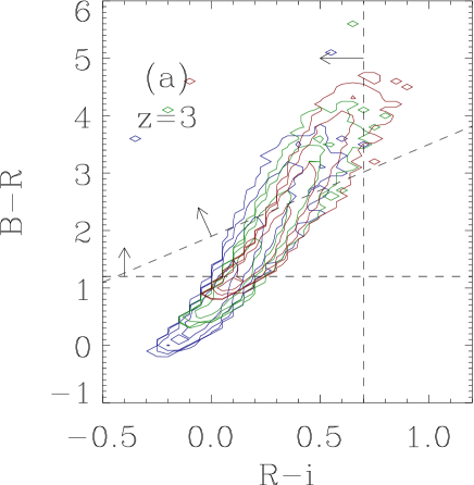
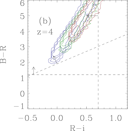
Figure 3: Colour-colour diagram for the plane of $B-R$ versus $R-i^{\prime}$. The selection criteria for $BRi$–LBGs in the Subaru survey are shown by the dashed lines. The contours in panels (a) and (b) show simulated galaxies in the ‘Large’ (G6) run for $z=3$ and $z=4$, respectively. Blue, green, and red contours correspond to $E(B-V)=0.0$, 0.15, and 0.30, respectively.

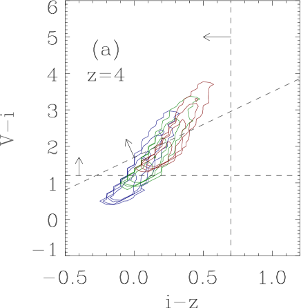
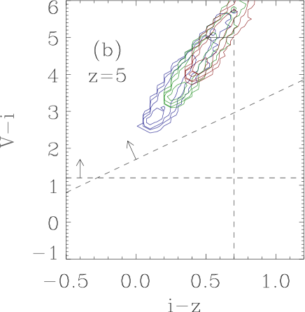
Figure 4: Colour-colour diagram for the plane of $V-i^{\prime}$ versus $i^{\prime}-z^{\prime}$. The selection criteria for $Viz$–LBGs in the Subaru survey are shown by the dashed lines. The contours in panels (a) and (b) show the simulated galaxies in the ‘Large’ (G6) run for $z=4$ and $z=5$, respectively. Blue, green, and red contours correspond to $E(B-V)=0.0$, 0.15, and 0.30, respectively.

LBGs are identified based on a significantly dimmer magnitude in a filter blueward of their Lyman break compared with a filter redward of their Lyman break. This difference is manifest as a significantly redder colour. Moreover, two filters redward of the Lyman break should not exhibit abnormal dropouts with respect to one another, a fact that can distinguish them from interlopers with very red spectra. Thus, in order to select LBGs from the sample, colour selection criteria are very important. For instance, galaxies at $z\approx 4$ will have Lyman breaks at approximately 4600Å, between the $B$ and $R$ filters (as shown in Fig. 1), so these galaxies will have large $B-R$ colours. But, we also expect them to have moderate $R-i^{\prime}$ colours, since both $R$ and $i^{\prime}$ are redward of 4600Å. The exact colour-colour selection criteria used by each survey are determined empirically by placing a sample of spectroscopically identified LBGs on a colour-colour diagram, or computing the track of local galaxies with known spectra (or artificial spectra of galaxies generated by a population synthesis model with assumed star formation histories) as a function of redshift.

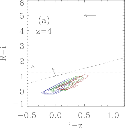
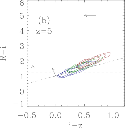
Figure 5: Colour-colour diagram for the plane of $R-i^{\prime}$ versus $i^{\prime}-z^{\prime}$. The selection criteria for $Riz$–LBGs in the Subaru survey are shown by the dashed lines. The contours in panel (a) and (b) show the simulated galaxies in the ‘Large’ (G6) run for $z=4$ and $z=5$, respectively. Blue, green, and red contours correspond to $E(B-V)=0.0$, 0.15, and 0.30, respectively.

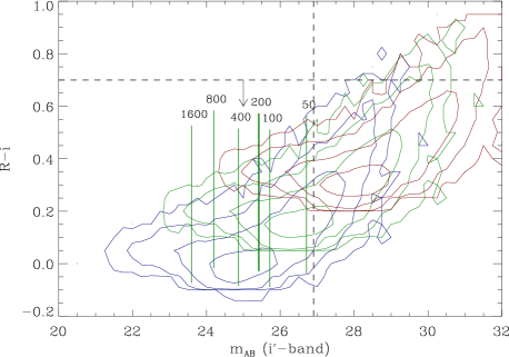
Figure 6: Colour-magnitude diagram for the ‘Medium’ boxsize (D5) run at $z=4$. Blue, green, and red contours outline the distribution of galaxies for $E(B-V)=0.0$, 0.15, and 0.30, respectively. Also shown in green are vertical lines approximately delineating the number of star particles in galaxies. Most galaxies found to the left of the first line comprise 1600 star particles or more, and 200 particles mark the end of our interval of confidence. Black dashed lines are cutoffs for $BRi$–LBGs as observed by the Subaru group. The vertical line indicates the $3\sigma$ limiting magnitude of $i^{\prime}=26.9$, and the horizontal line represents one of the colour-colour selection criteria used to identify LBGs.

For example, Ouchi et al. (2004) use the following colour criteria for selecting $z\sim 4$ galaxies:

$$\hskip 56.9055ptB-R > 1.2$$ (5)

$$\hskip 56.9055ptR-i^{\prime} < 0.7$$ (6)

$$\hskip 56.9055ptB-R > 1.6(R-i^{\prime})+1.9$$ (7)

Galaxies identified as LBGs by these criteria are called $BRi$–LBGs. Similar criteria exist for $V-i$’ versus $i^{\prime}-z^{\prime}$ colours, and $R-i^{\prime}$ versus $i^{\prime}-z^{\prime}$ colours; galaxies selected in this way are called $Viz$–LBGs and $Riz$–LBGs, respectively. Each of these three classes of LBGs corresponds to an approximate range in redshift space. The central redshifts for $BRi$, $Viz$, and $Riz$ populations are approximately 4, 5, and 5, respectively. The $Riz$ selection has a narrower range of redshift than the $Viz$ selection, so we will use the $BRi$ sample to compare to our $z=4$ simulations, and $Riz$ sample to compare to our $z=5$ simulations.

In Figs. 3 – 5, we show the colour-colour diagrams of our simulated galaxies. Overall, the agreement with the observation is good, and the simulated galaxies fall within the same region as the observed galaxies, a conclusion consistent with Nagamine et al. (2004d). Very few $z=3$ galaxies in our simulation would be detected as $BRi$–LBGs, but a large fraction of $z=4$ galaxies would. Similarly, relatively few $z=4$ galaxies in our simulations would be detected as $Viz$–LBGs or $Riz$–LBGs compared with $z=5$ galaxies. This result appears to be relatively insensitive to the amount of Calzetti extinction, at least for the range of extinction values we considered.

In Fig. 6, we also show the colour–magnitude diagram on the plane of $i^{\prime}$-band apparent magnitude and $R-i^{\prime}$ colour for the ‘Medium’ (D5) run. This figure shows that all the simulated galaxies brighter than $m_{AB}(i^{\prime}-{\rm band})=27$ satisfy the colour-selection of $R-i^{\prime}<0.7$. Since the brightest galaxies in the simulations are the most massive ones, this means that the LBGs in the simulations are the brightest and most massive galaxies with $E(B-V)\sim 0.15$ at each epoch. The situation of course changes when a larger value of extinction is allowed, as such galaxies could become redder than $R-i^{\prime}=0.7$. Such dusty starburst galaxies may exist in the real universe, but we are not considering them in this paper by restricting ourselves to $E(B-V)\leq 0.3$.

5 Galaxy stellar masses

Fig. 7 shows stellar mass $M_{\star}$ vs. UV magnitude for the simulated galaxies over several redshifts and for different extinction values, in relation to the survey limiting magnitudes. From the figure it is seen that the ‘Large’ box size simulation contains galaxies as massive as $M_{\star}\sim 10^{11}{h_{70}^{-1}}{M_{\odot}}$ at $z=6$, and $M_{\star}\sim 10^{11.7}{h_{70}^{-1}}{M_{\odot}}$ at $z=3$. Larger objects are too rare to be found in a simulation of this size. The diagonal lines in the figure depicting mass-to-light ratio show that this value is generally increasing going from higher to lower redshift, so that the luminosity per stellar mass is decreasing with time.

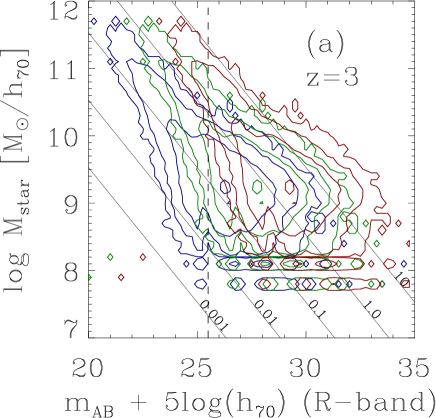
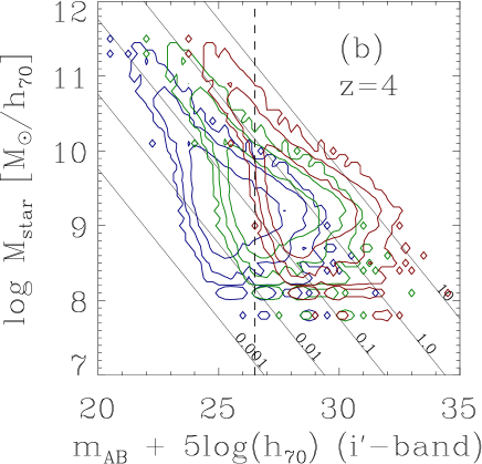
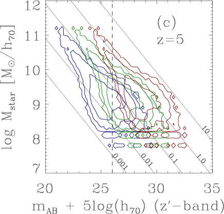
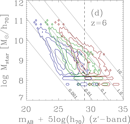
Figure 7: Contour plots of stellar mass of galaxies vs. UV magnitude, for redshifts $z=3-6$, using the ‘Large’ (solid colour contour) box size. Blue, green, and red contours represent extinctions of $E(B-V)=0.0$, 0.15, and 0.3 respectively. The dashed black lines indicate the magnitude limits of Steidel et al. (2003) at $z=3$, the SDF sample for $z=4$ and 5, and the HST GOODS for $z=6$. Diagonal lines show lines of constant stellar mass to light ratio; the value of $M_{\star}/(\lambda L_{\lambda})$ is labeled for each line, in units of $M_{\odot}/L_{\odot}$.

Fig. 8 shows the cumulative number density (integral of the luminosity function for galaxies brighter than a certain magnitude limit) of galaxies at various redshifts and for different extinction values for the ‘Large’ (solid curves) and ‘Medium’ (dashed curves) box sizes. Every simulation of limited size will underpredict the continuum value by a certain amount, depending on the bright-end cutoff imposed by the finite volume, so it is not surprising that the ‘Medium’ simulation gives systematically lower densities than the ‘Large’ simulation. For comparison, we show values determined by Adelberger et al. (2003) at $z=3$, Ouchi et al. (2004) at $z=4$ and 5, and Bouwens et al. (2004) at $z=6$. The best match with the observations is reached for $E(B-V)=0.15$ at $z=3$, but the required extinction appears to slightly increase towards $E(B-V)=0.3$ at higher redshifts.

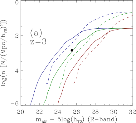
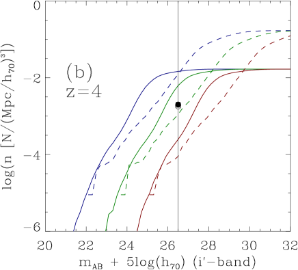
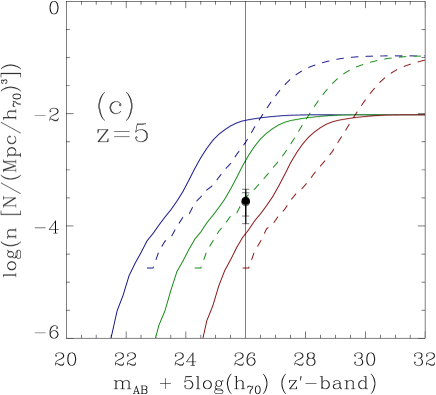
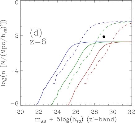
Figure 8: Total number density of galaxies below a threshold magnitude in the ‘Large’ box size (G6 run, solid curves) and ‘Medium’ box size (D5 run, dashed curves) simulations. Blue, green, and red curves represent the extinction values $E(B-V)=0.0$, 0.15, and 0.3, respectively. The vertical solid black lines roughly represent the magnitude limits of the Steidel et al. (2003) sample for $z=3$, the SDF sample for $z=4$ and 5, and the HST GOODS for $z=6$.

At $z=3$ and for $E(B-V)=0.15$, we find a value for the number density of $n(R<25.5)\sim 1\times 10^{-3}({h_{70}^{-1}}{\rm Mpc})^{-3}$. This magnitude was determined by the limiting magnitude in the survey of Adelberger et al. (2003); for values at different magnitudes, refer to Fig. 8. Similarly, at $z=4$ and 5, we determine values of $n(i^{\prime}<26.5)\sim 6\times 10^{-3}({h_{70}^{-1}}{\rm Mpc})^{-3}$ and $n(z^{\prime}<26.0)\sim 1.5\times 10^{-3}({h_{70}^{-1}}{\rm Mpc})^{-3}$. The variation in these results primarily reflects the different limiting magnitudes of Ouchi et al. (2004) instead of an internal evolution of the LF over this redshift range. Finally, at $z=6$, we measure a value of $n(z^{\prime}<29.0)\sim 2.1\times 10^{-2}({h_{70}^{-1}}{\rm Mpc})^{-3}$, where the limiting magnitude was chosen as in Bouwens et al. (2004).

6 Luminosity Functions

The most widely used analytic parameterisation of the galaxy luminosity function is the Schechter Function (Schechter, 1976), the logarithm of which is given by

$$\log(\Phi(M))=\log(0.4\ln(10)\Phi^{*})+\mu(\alpha+1)-10^{\mu}/\ln(10),$$ (8)

where $\mu=-0.4(M-M^{*})$, and $\Phi^{*}$, $M^{*}$, and $\alpha$ are the normalisation, characteristic magnitude, and faint-end slope, respectively. We note that throughout this section, we plot luminosity functions (LFs) in terms of magnitude rather than luminosity. Brighter objects will thus appear farther left on the abscissa than fainter objects.

The LF measured from our simulations suffers both from boxsize and resolution effects, so we expect it to be physically meaningful only for a certain limited range of luminosities. At the faint end, objects are made up by a relatively small number of particles, and may not be well-resolved, and even smaller objects will be lost entirely. In our simulations, the luminosity functions generally have a peak at around 100 stellar particles. The turn-over on the dim side of this peak owes to the mass resolution. In order to avoid being strongly affected by this limitation, we usually discard results based on galaxies with fewer than 200 stellar particles.

At the bright end, objects become increasingly rare. When there is only of order one object per bin in the entire box, the statistical error of the LF dominates and we cannot reliably estimate the abundance. In order to improve the sampling of these objects, a larger simulation volume needs to be chosen, which is however in conflict (for a given particle number) with the usual desire to obtain a good mass resolution.

Fig. 9 illustrates these numerical limitations and defines a region where the LF results can be trusted. The cut-offs we indicated here are however approximate. A precise determination of the interval over which the measured LF is physically significant requires running many simulations with successively higher resolution, and looking for an interval of convergence. Such a programme was carried out by Springel & Hernquist (2003b) in their study of the cosmic star formation rate. We here analyse three different box sizes taken from their set of simulations, yielding a good coverage of magnitude space. Where appropriate, we also combine these results to obtain a measurement covering a larger dynamic range. In subsequent figures, the approximate interval of physical significance for the LF measurements will be shown with a thicker line than the rest of the curve. Strictly speaking, it is only this interval that can be compared reliably with observations.

Figure 9: Typical luminosity function, depicting our approximate criterion for physical relevance of the data, and uncertainty. The top and right axes show simulation-based measurements of objects: the approximate number of stellar particles which make up an object in the given magnitude bin, and the number of objects in the entire box in a given magnitude bin (of size 0.2 mags). The bottom and left axes are the corresponding physical measurements: the magnitude as derived from the spectrum of the objects, and the number density as a luminosity function. A fiducial cutoff of 200 stellar particles is chosen as the lower limit for accurately resolved objects, although this value is somewhat arbitrary. The dotted line indicates Poisson $\sqrt{N}$ uncertainties, and the dashed line indicates the standard deviation of the mean between the luminosity function derived for eight disjoint sub-regions of the entire box. Since the latter uncertainty is greater throughout most of the range, only it is shown on subsequent plots. Both forms of uncertainty are dependent on the bin size, 0.2 mags.

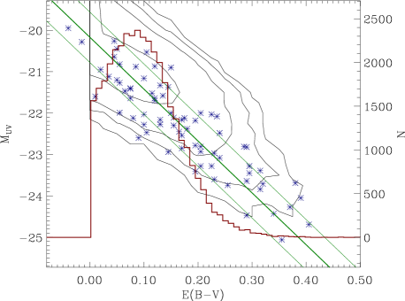
Figure 10: Correlation between UV magnitude and extinction value $E(B-V)$. Blue points, plotted with respect to the left axis, show the original data from Shapley et al. (2001). Green lines show the best linear fit to the data, and the lines denote 1-$\sigma$ scatter. Black contours outline the extinction values we assigned to the simulated galaxies using the procedure described in Section 6 (for the ‘Large’ boxsize G6-run at $z=4$) in order to match up with this correlation. The red histogram, plotted with respect to the right axis, shows the distribution of extinction values of the black contours. However, for the reasons described in the text, we do not use this method of assigning variable $E(B-V)$ hereafter.

Also shown in Fig. 9 is the estimated uncertainty in the LF owing to sample size, which we estimated in two ways. First, we calculated $\sqrt{N}$ Poisson statistical errors, simply by taking the square root of the number of objects in each bin. Second, we divided the box into eight octants, and computed the standard deviation of the mean between the LFs computed with each of the eight octants. In all cases, the second method produced larger uncertainty over the interval of physical significance, indicating that the ‘cosmic variance’ error owing to our limited boxsize exceeds a simple Poisson estimate. We therefore use error estimates obtained with the octant method in our subsequent figures on the LF results and ignore the Poisson errors.

Typically, we assumed three values for the extinction, $E(B-V)=0.0$, 0.15, and 0.30, and produced LF-estimates for them separately. In this procedure, we hence always assigned a single extinction value to every galaxy for which we computed magnitudes. However, in the real universe we instead expect a distribution of extinction values (e.g., Shapley et al., 2001; Ouchi et al., 2004), which could be quite broad. This prompted us to explore possible effects owing to a ‘variable extinction’. To this end, we first introduced random scatter into the values for extinction: Instead of appling the same extinction to all galaxies, each galaxy was assigned an individual value of $E(B-V)$ determined by a Gaussian random variable with a mean of 0.15 and a standard deviation of 0.10. Moreover, a cutoff was imposed so that no galaxy had a negative extinction value. We found that such variable scatter tends to smooth out the luminosity function somewhat, as expected, but it does not produce results readily distinguishable from a uniform extinction value.

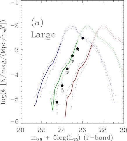
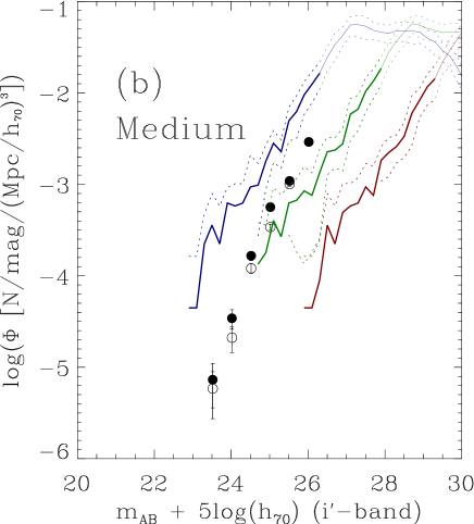
Figure 11: $i^{\prime}$-band luminosity function for both ‘Large’ (G6, panel a) and ‘Medium’ boxsize (D5, panel b) simulation runs at $z=4$, and the observational data for $BRi$–LBGs (Ouchi et al., 2004, Fig. 16). Simulation LFs are plotted as blue, green, and red curves representing extinction values of $E(B-V)=0.0$, 0.15, and 0.30, respectively. The Subaru survey data are shown as black crosses and boxes for the two different survey fields (Ouchi et al., 2004, Fig. 16).

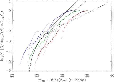
Figure 12: Luminosity function for all three boxsizes at $z=4$. Extinction colour-coding is the same as in the previous plots. Solid and dashed lines are best Schechter fits to Subaru $BRi$–LBG data, assuming a value for the faint-end slope of $\alpha=-2.2$ and -1.6, respectively (Ouchi et al., 2004, Fig. 16). The dashed-dotted line has a slope of -2.0, but is not a fit to the Subaru data.

There is evidence for a correlation between UV magnitude and extinction. In particular, Shapley et al. (2001) found that, over the magnitude range studied, dust obscures almost exactly enough flux to give all galaxies a similar apparent magnitude. The data from Shapley et al. (2001), along with the extinction values we adopted to emulate it, appear in Fig. 10. When these extinction values are used, brighter galaxies have larger values of $E(B-V)$. The effect of this distribution of extinction values is such that the brightest galaxies become dim enough to agree with the observed magnitudes, while the fainter ones suffer little extinction so that they agree with the narrow range of observed magnitude. Taken together, this effect produces a simulated LF that matches the empirical one quite well within the observed range of magnitudes, requiring only moderate extinction at the faint end. However, invoking variable extinction in this manner is of course bound to succeed at some level, because we here ‘hide’ the difference between simulated and observed LFs in the variable extinction law. While such a law in principle may exist, we prefer here to systematically study the effect of extinction by assuming different values of $E(B-V)$ uniformly for the entire sample.

In Figs. 11 through 15, we show the LFs derived from the simulated observations as coloured curves with data points from observational surveys overplotted. These are the main results of this paper. We first compare the $i^{\prime}$-band LFs directly to the observations. For $z=4$, this is shown in Fig. 11 for the ‘Large’ (G6) and ‘Medium’ boxsize (D5) runs, along with data from Ouchi et al. (2004). The observational data points do not extend faint enough to offer any overlap with the ‘Small’ (Q5 & Q6) run’s LF, therefore we do not show the results from the ‘Small’ simulation in this figure. As seen in the figures, the data points are roughly consistent with the green curves, corresponding to an extinction value of $E(B-V)\sim 0.15$. The result of our ‘Large’ run covers the entire range of the observed magnitude ranges, but the ‘Medium’ run overlaps only with the fainter side of the Subaru data because of the moderate simulation volume.

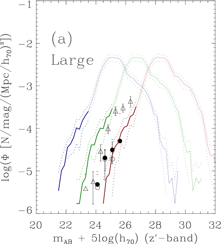
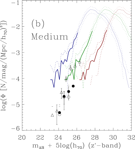
Figure 13: $z^{\prime}$-band luminosity function for both ‘Large’ (G6, panel a) and ‘Medium’ boxsize (D5, panel b) simulations at $z=5$. Survey results for similar redshifts are shown with symbols. Simulation data are plotted as blue, green, and red curves representing extinction values of $E(B-V)=0.0$, 0.15, and 0.30, respectively. Ouchi et al.’s $z^{\prime}$-band survey data are shown as black crosses and boxes for the two different survey fields (Ouchi et al., 2004, Fig. 16). The updated $I$-band survey data of Iwata et al. (2004) are shown as triangles.

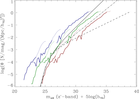
Figure 14: $z^{\prime}$-band luminosity function for all three boxsizes at $z=5$. Extinction colour-coding is the same as in the previous plots. Solid and dashed lines are best fit Schechter functions to Subaru $Riz$–LBG data, assuming a value for the faint-end slope of $\alpha=-2.2$ and $-1.6$, respectively (Ouchi et al., 2004, Fig. 16). The dashed-dotted line has a slope of $-2.0$, but is not a fit to the data.

We then compared the simulated LFs for all three boxsizes (‘Large’, ‘Medium’, and ‘Small’) to the best-fitting Schechter function as determined from the Subaru survey. For $z=4$, this is shown in Fig. 12. The two Schechter functions plotted in this figure correspond to the best fit to the Subaru data obtained by Ouchi et al. (2004) with a fixed faint-end slope of either $\alpha=-1.6$ (dashed line) or $-2.2$ (solid line). The simulated LF with $E(B-V)=0.15$ is consistent with the faint-end slope between these two values, and the value of $\alpha=-2.0$ (dash-dotted line) appears reasonable.

Similar results emerged for $z=5$. In Fig. 13, we show the ‘Large’ and ‘Medium’ boxsize LFs and compare them with data from Ouchi et al. (2004) and Iwata et al. (2004). At $z=5$, the survey data appear to be more consistent with the simulations using $E(B-V)=0.3$, particularly at the bright end, suggesting a slightly larger extinction at $z=5$ than at $z=4$. And again, when all three boxsizes are plotted along with the best-fitting Schechter function in Fig. 14, the most consistent value for the faint end slope $\alpha$ appears to lie between $-1.6$ and $-2.2$. Note that there are small discrepancies between the LF-estimates by Ouchi et al. (2004) and Iwata et al. (2004). This may owe to slight differences in the colour-selection criteria used in the two surveys.

In Fig. 15, we compare the UV-magnitude LFs at $z=6$ in the ‘Large’ and ‘Medium’ boxsize simulations to data from Bouwens et al. (2004) . Again, a value of $E(B-V)$ between 0.15 and 0.30 leads to the best match with the data, and an extinction with $E(B-V)=0.15$ is favoured based on this comparison.

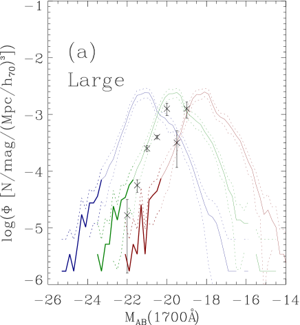
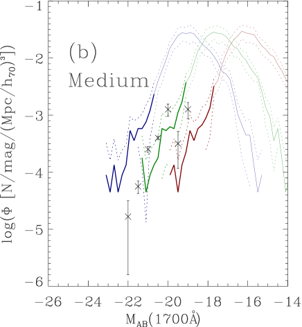
Figure 15: UV luminosity function at $z=6$ for both ‘Large’ and ‘Medium’ boxsize simulations and the observational data from Bouwens et al. (2004, black crosses). Simulation data are plotted as blue, green, and red curves, representing extinction values $E(B-V)=0.0$, 0.15, and 0.30, respectively.

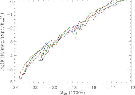
Figure 16: Rest frame UV luminosity function for all three boxsizes for redshifts $z=6$ (red), 5 (orange), 4 (green), and 3 (blue). For clarity, results for each LF are only plotted over the reliable range, and error bars are omitted. The extinction value for all curves is here $E(B-V)=0.15$.

Finally, Fig. 16 examines the evolution of the LF over the redshift range studied. To this end, we plot all redshifts for all boxsizes using the single extinction value $E(B-V)=0.15$. Overall, the LF of our simulations shows little if any evolution over the redshift range in question. The absence of strong evolution is probably related to the fact that the evolution of the cosmic star formation rate (SFR) density is quite mild from $z=3$ to 6 in our simulations, as discussed by Springel & Hernquist (2003b) and Hernquist & Springel (2003). In both SPH and total variation diminishing (TVD) simulations (Nagamine et al., 2004), the cosmic SFR continues to rise gradually from $z=3$ to 5, and peaks at $z=5-6$. Nagamine et al. (2005a) have shown that the evolution of the LF from $z=3$ to $z=2$ is about 0.5 mag, so it is perhaps not too surprising that the evolution at higher redshift is of comparably small size. Note that in terms of proper time, the redshift interval from $z=6$ to 3 is only about as long as the interval from $z=3$ to 2.

7 Discussion & Conclusions

Using state-of-the-art cosmological SPH simulations, we have derived the colours and luminosity functions of simulated high-redshift galaxies and compared them with observations. In particular, we have employed a series of simulations with different boxsizes and resolution to identify the effects of numerical limitations. We find that the colours of galaxies at $z=4-6$ agree with the observed ones on the colour-colour planes used in observational studies, and our results confirm the generic conclusion from earlier numerical studies (Nagamine, 2002; Weinberg et al., 2002; Nagamine et al., 2004d, 2005a) that UV bright LBGs at $z\geq 3$ are the most massive galaxies with $E(B-V)\sim 0.15$ at each epoch.

The simulated LFs are in good agreement with the data provided an extinction of $E(B-V)=0.15-0.30$ is assumed. The faint-end slope of our results is consistent with a value between $\alpha=-1.6$ and $-2.2$, as found with the Subaru data (Ouchi et al., 2004). The simulated LFs best match a very steep faint-end slope of $\alpha\sim-2.0$. The recent analysis of Hubble Space Telescope Ultra Deep Field (UDF) data by Yan & Windhorst (2004) also suggests a quite steep faint-end slope of $\alpha=-1.8$ to $-1.9$, in good agreement with the simulations.

The steep faint-end slopes at $z\ga 6$ found here are interesting because they have significant implications for the history of the reionisation of the Universe. As discussed by, e.g., Springel & Hernquist (2003b), Yan & Windhorst (2004), and Cen et al. (2005), it may be possible to reionise the Universe at $z=6$ with ionising photons from Population II stars in normal galaxies alone if the faint-end slope of the galaxy luminosity function is sufficiently steep ($\alpha\la-1.6$). Note that Nagamine et al. (2004d) also found a similarly steep faint-end slope at $z=3$ in the same SPH simulations.

The suggestion that the faint-end slope may be much steeper at high redshifts than in the Local Universe is intriguing, and the agreement between the recent observations and our simulations lends encouraging support for this proposal. However, this immediately invokes the question of what mechanisms changed the LF over time and gave it the shallow slope ($\alpha\sim-1.2$) observed locally in the 2dF (Cole et al., 2001) and SDSS surveys (Blanton et al., 2001). A similarly strong flattening does not occur in our simulations (Nagamine et al., 2004d), but this could owe to an incomplete modeling of the physics of feedback processes from supernova and quasars. We note that the SPH simulations employed in this paper already included a galactic wind model (see Springel & Hernquist, 2003a, for details) which drives some gas out of low-mass halos, but the effect is not sufficiently sensitive to galaxy size to produce a significantly flattened faint-end slope. The shallowness of the faint-end slope of the local LF hence remains a challenge for cosmological simulations and may point to the need for other physical processes, such as black hole growth (e.g., Springel et al., 2005b; Di Matteo et al., 2005; Robertson et al., 2005).

In light of this, it is therefore particularly encouraging that the simulations are more successful at high redshift. The steep faint-end slope found by observations in this regime is an important constraint on the nature of the feedback processes themselves. Presently, the observational results still bear substantial uncertainties, however, stemming mostly from their limited survey volume which makes them prone to cosmic variance errors, and less from the faintness levels reached, which already probe down to $m_{AB}=29$ magnitude in the case of the UDF survey. The next generation of wide and deep surveys will shed more light on this question in the near future.

References

- Adelberger et al. (2003) Adelberger K. L., Steidel C. C., Shapley A. E., Pettini M., 2003, ApJ, 584, 45
- Baugh et al. (1998) Baugh C. M., Cole S., Frenk C. S., Lacey C. G. 1998, ApJ, 498, 504
- Blaizot et al. (2004) Blaizot J., Guiderdoni B., Devriendt J. E. G., Bouchet F. R., Hatton S. J., Stoehr F. 2004, MNRAS, 352, 571
- Blanton et al. (2001) Blanton M. R. et al., 2001, AJ, 121, 2358
- Bouwens et al. (2004) Bouwens R. J. et al., 2004, ApJ, 606, L25
- Bruzual & Charlot (2003) Bruzual G., Charlot S., 2003, MNRAS, 344, 1000
- Calzetti et al. (2000) Calzetti D., Armus L., Bohlin R., Kinney A., Koornneef J., Storchi-Bergmann T., 2000, ApJ, 533, 682
- Cen et al. (2005) Cen R., Nagamine K., Hernquist L., Ostriker J. P., Springel V., 2005, ApJ, in preparation
- Cole et al. (2001) Cole S. et al., 2001, MNRAS, 326, 255
- Davé et al. (1999) Davé R., Hernquist L., Katz N., Weinberg D. H., 1999, ApJ, 511, 521
- Dickinson et al. (2004) Dickinson M. et al. 2004, ApJ, 600, L99
- Di Matteo et al. (2005) Di Matteo T., Springel V., Hernquist L., 2005, Nature, 433, 604
- Finlator et al. (2005) Finlator K., Davé R., Papovich C., Hernquist L., 2005, ApJ, submitted (astro-ph/0507719)
- Fukugita et al. (1995) Fukugita M., Shimasaku K., Ichikawa T., 1995, PASP, 107, 945
- Furlanetto et al. (2004a) Furlanetto S. R., Schaye J., Springel V., Hernquist L., 2004a, ApJ, 606, 221
- Furlanetto et al. (2004b) Furlanetto S. R., Sokasian A., Hernquist L., 2004b, MNRAS, 347, 187
- Furlanetto et al. (2004c) Furlanetto S. R., Zaldarriaga M., Hernquist L., 2004c, ApJ, 613, 16
- Furlanetto et al. (2004d) Furlanetto S. R., Zaldarriaga M., Hernquist L., 2004d, ApJ, 613, 1
- Giavalisco et al. (2004) Giavalisco M. et al., 2004, ApJ, 600, L103
- Haardt & Madau (1996) Haardt F., Madau P., 1996, ApJ, 461, 20
- Harford & Gnedin (2003) Harford A. G., Gnedin N. Y., 2003, ApJ, 597, 74
- Hernquist (1993) Hernquist L., 1993, ApJ, 404, 717
- Hernquist & Springel (2003) Hernquist L., Springel V., 2003, MNRAS, 341, 1253
- Iwata et al. (2004) Iwata I. et al., in de Grijs R., Gonzalez D. R. M., eds, Astrophys. Space Sci. Libr. Vol. 329, Starbursts: From 30 Doradus to Lyman Break Galaxies. Dordrecht: Springer, Cambridge, p.29
- Katz et al. (1996) Katz N., Weinberg D. H., Hernquist L., 1996, ApJS, 105, 19
- Lowenthal et al. (1997) Lowenthal J. et al., 1997, ApJ, 481, 673
- Madau (1995) Madau P., 1995, ApJ, 441, 18
- Mihos & Hernquist (1996) Mihos J. C., Hernquist L., 1996, ApJ, 464, 641
- Miyazaki et al. (2002) Miyazaki S. et al., 2002, PASJ, 54, 833
- Nagamine (2002) Nagamine K., 2002, ApJ, 564, 73
- Nagamine et al. (2004) Nagamine K., Cen R., Hernquist L., Ostriker J. P., Springel V., 2004, ApJ, 610, 45
- Nagamine et al. (2005a) Nagamine K., Cen R., Hernquist L., Ostriker J. P., Springel V., 2005a, ApJ, 618, 23
- Nagamine et al. (2005b) Nagamine K., Cen R., Hernquist L., Ostriker J. P., Springel V., 2005b, ApJ, 627, 608
- Nagamine et al. (2004a) Nagamine K., Springel V., Hernquist L., 2004a, MNRAS, 348, 421
- Nagamine et al. (2004b) Nagamine K., Springel V., Hernquist L., 2004b, MNRAS, 348, 435
- Nagamine et al. (2004c) Nagamine K., Springel V., Hernquist L., Machacek M., 2004c, MNRAS, 355, 638
- Nagamine et al. (2004d) Nagamine K., Springel V., Hernquist L., Machacek M., 2004d, MNRAS, 350, 385
- O’Shea et al. (2005) O’Shea B.W., Nagamine K., Springel V., Hernquist L., Norman M.L., 2005, ApJ, submitted (astro-ph/0312651)
- Ouchi et al. (2004) Ouchi M. et al., 2004, ApJ, 611, 660
- Robertson et al. (2005) Robertson B., Hernquist L., Bullock J. S., Cox T. J., Matteo T. D., Springel V., Yoshida N., 2005, ApJ, submitted (astro-ph/0503369)
- Schechter (1976) Schechter P., 1976, ApJ, 203, 297
- Shapley et al. (2001) Shapley A., Steidel C., Adelberger K., Dickinson M., Giavalisco M., Pettini M., 2001, ApJ, 562, 95
- Somerville et al. (2001) Somerville R. S., Primack J. R., Faber S. M., 2001, MNRAS, 320, 504
- Springel (2005) Springel V., 2005, MNRAS, submitted (astro-ph/0505010)
- Springel & Hernquist (2002) Springel V., Hernquist L., 2002, MNRAS, 333, 649
- Springel & Hernquist (2003a) Springel V., Hernquist L., 2003a, MNRAS, 339, 289
- Springel & Hernquist (2003b) Springel V., Hernquist L., 2003b, MNRAS, 339, 312
- Springel et al. (2005b) Springel V., Di Matteo T., Hernquist L., 2005, ApJ, 620, L79
- Steidel & Hamilton (1993) Steidel C. C., Hamilton D., 1993, AJ, 105, 2017
- Steidel et al. (1999) Steidel C. C., Adelberger K. L., Giavalisco M., Dickinson M., Pettini M., 1999, ApJ, 519, 1
- Steidel et al. (2003) Steidel C. C., Adelberger K. L., Shapley A. E., Pettini M., Dickinson M., Giavalisco M., 2003, ApJ, 592, 728
- Weinberg et al. (2002) Weinberg D. H., Hernquist L., Katz N., 2002, ApJ, 571, 15
- Yan & Windhorst (2004) Yan H., Windhorst R. A., 2004, ApJ, 612, L93