Number ratios of young stellar objects in embedded clusters

Embedded clusters usually contain young stellar objects in different evolutionary stages. We investigate number ratios of objects in these classes in the star-forming regions $\rho$ Ophiuchi, Serpens, Taurus, Chamaeleon I, NGC 7129, IC 1396A, and IC 348. They are compared to the temporal evolution of young stars in numerical simulations of gravoturbulent fragmentation in order to constrain the models and to possibly determine the evolutionary stage of the clusters. It turns out that Serpens is the youngest, and IC 348 the most evolved cluster, although the time when the observations are best represented varies strongly depending on the model. Furthermore, we find an inverse correlation of the star formation efficiency (SFE) of the models with the Mach number. However, the observational SFE values cannot be reproduced by the current isothermal models. This argues for models that take into account protostellar feedback processes and/or the effects of magnetic fields.

1 Introduction

Almost all stars form in clusters. Embedded clusters contain various types of young stars, making them ideal laboratories to study star formation as they provide a large and genetically homogeneous sample (see Lada & Lada lada_lada (2003) for a review).

Four classes of young stellar objects (YSOs) are distinguished according to the properties of their spectral energy distributions (SEDs). Originally Lada (1987IAUS..115….1L (1987)) defined Class 1, 2, and 3 objects according to the slope in the SED from 1 to 20 $\mu$m. Note that Class 2 sources correspond to classical T Tauri stars and Class 3 objects to weak line T Tauri stars. Later the extremely embedded sources (Class 0 objects) were added to this classification, and their observational properties are defined e.g. in André et al. (andre00 (2000)). These four classes are interpreted as an evolutionary sequence from Class 0 to 3. There are, however, concerns that some Class 0 sources might be mimicked by Class 1 objects seen edge on (Men’shchikov & Henning men_henn97 (1997)). Furthermore there are works suggesting that Class 2 and Class 3 objects are actual of the same age (e.g. Walter 1986ApJ…306..573W (1986)). Class 0 sources are deeply embedded protostars, possessing a large sub-mm ($\lambda>$ 350 $\mu$m) to bolometric luminosity ratio (L_smm/L${}_{\rm bol}>$ 0.005). The Class 0 stage is the main accretion phase and lasts only a few 10⁴ yr. Class 1 objects are relatively evolved protostars. They are surrounded by an accretion disc and a circumstellar envelope. Pre-main-sequence stars in Class 2 and 3 are characterised by a circumstellar disc (optically thick in Class 2, optically thin in Class 3) and the lack of a dense circumstellar envelope. The progenitors of these forming stars are prestellar cores (starless cores, prestellar condensations). These are gravitationally bound, dense molecular cloud cores with typical stellar masses that may already be in a state of collapse, but have not formed a central protostellar object yet.

Star formation in molecular clouds is controlled by the complex interplay between interstellar turbulence and self-gravity (Vázquez-Semadeni et al. VS_etal00 (2000); Larson larson03 (2003); Mac Low & Klessen maclow_klessen04 (2004), and references therein). The supersonic turbulence ubiquitously observed in Galactic molecular gas (Blitz blitz93 (1993)) generates strong density fluctuations with gravity taking over in the densest and most massive regions (e.g., Sasao sasao73 (1973); Hunter & Fleck hunter_fleck82 (1982); Elmegreen elmegreen93 (1993); Padoan padoan95 (1995); Klessen klessen01 (2001); Padoan & Nordlund padoan_nordlund02 (2002)). We call this process gravoturbulent fragmentation. In a cloud core where gravitational attraction overwhelms all opposing forces from pressure gradients or magnetic fields, localised collapse will set in. The density increases until a protostellar objects forms in the centre and grows in mass via accretion from the infalling envelope. The gravoturbulent models of molecular cloud evolution discussed here can describe the entire collapse of a cloud core and the build-up of a stellar cluster as a function of time (see, e.g., Klessen et al. KHM00 (2000); Klessen klessen01 (2001); Heitsch et al. HMK01 (2001); Schmeja & Klessen sk04 (2004); Jappsen & Klessen JK04 (2004)). These models provide a “snapshot” of the cluster at any time, allowing the comparison with observed clusters, and possibly the determination of the cluster’s evolutionary status according to the models. This permits to constrain the models and possibly to determine the evolutionary stage of the star-forming region by comparison with the models.

Complete unbiased surveys of clusters for the content of all four evolutionary classes and prestellar cores are difficult to undertake, since they require different observational techniques. Hence, different investigations have to be combined. The result therefore might suffer from different detection limits or varying spatial coverage. With this caveat in mind, we search the literature for information on the different YSO classes in several star-forming regions and tried to construct roughly homogeneous samples of Class 0 to Class 3 sources and prestellar cores to compare them with our models.

The purpose of this paper is twofold: On the one hand, we compile an observational sample of absolute numbers of YSOs belonging to the different classes for several star-forming regions from the literature (Sect. 2), on the other hand we analyse the evolution of the YSO classes in gravoturbulent models (Sect. 3) and compare it with the observational data in Sect. 4. Finally, in Sect. 5 we summarise and conclude our findings.

2 Observational data

The detection and classification of prestellar cores and Class 0/1/2/3 objects requires different observational techniques. Thus, we have to construct our samples from various sources. We consider corresponding areas on the sky, but the caveat remains that the combined samples may be far from complete and not homogeneous. Since it would hardly effect the relative numbers, the problem of unresolved binaries can be neglected. Besides, we cannot resolve close binaries in the SPH models either. The absolute and relative numbers of YSOs adopted from the observations for the subsequent analysis are listed in Table 1. Prestellar cores are hard to determine both from observations and in our models, and in particular they are hard to compare, since the status of the cores (Jeans-critical or subcritical) is often unknown. Some cores considered as “starless” might even in fact turn out to harbour embedded sources (Young et al. young04 (2004)). Therefore we do not use them for the actual comparison, but keep them as an additional test for consistency. Due to constraints from the models (see Sect. 3) we consider Class 2 and 3 combined. So in the lower panel of Table 1 only Class 0, Class 1, and the combined set of Class 2+3 objects are shown.

2.1 $\rho$ Ophiuchi

The $ρ$~Ophiuchi molecular cloud is the closest and probably best-studied star-forming region, offering the most complete sample of YSOs. Bontemps et al. (bontemps01 (2001)) find a total number of 16 Class 1 sources, 123 Class 2 sources, 38 Class 3 sources, and 39 Class 3 candidates. They did not detect the previously known two Class 0 objects lying within their area. Following the reasoning of Bontemps et al. (bontemps01 (2001)) and the findings of Grosso et al. (grosso00 (2000)) that there might be almost as many Class 3 as Class 2 objects, we add the candidates to the Class 3 sample, yielding a total number of 77 Class 3 sources. Stanke et al. (stanke04 (2004)) performed a 1.2 mm dust continuum survey of the $\rho$ Oph cloud and detected 118 starless clumps and a couple of previously unknown protostars. To obtain a reasonably homogeneous sample when combining the Bontemps et al. (bontemps01 (2001)) and Stanke et al. (stanke04 (2004)) surveys we restrict ourselves to the range covered by both investigations, which is the $45^{\prime}\times 45^{\prime}$ region of the main $\rho$ Oph cloud (L1688) investigated by Bontemps et al. (bontemps01 (2001)). This area contains two Class 0 sources (Froebrich froebrich04 (2005); Stanke et al. stanke04 (2004)). The global star formation efficiency (SFE) in L1688 is estimated at $6-14\%$, although the local SFE in the subclusters where active star formation takes place is significantly higher with $\sim 31\%$ (Bontemps et al. bontemps01 (2001)). The measured velocity dispersion is $2.6\leavevmode\nobreak\ \mathrm{km\leavevmode\nobreak\ s}^{-1}$ in $\rho$ Oph A and $2.7\leavevmode\nobreak\ \mathrm{km\leavevmode\nobreak\ s}^{-1}$ in $\rho$ Oph B (Kamegai et al. kamegai03 (2003)). With the reported temperatures of 11 and 7.8 K this corresponds to Mach numbers of $\mathcal{M}\approx 13.5$ and $\mathcal{M}\approx 15.5$, respectively.

Table 1: Absolute (upper panel) and relative (lower panel) numbers of YSOs of different classes from observations (references see text)

Region	prestellar	0	1	2	3
$\rho$ Oph	98	2	15	111	77
Serpens	26	5	19	18	$\sim$20
Taurus	52	3	25	108	72
Cha I	$<$71	2	5	175
IC 348		2	2	261
NGC 7129		1	20	80
IC 1396A		2	6	47	1
$\rho$ Oph		0.01	0.07	0.92
Serpens		0.08	0.31	0.61
Taurus		0.01	0.12	0.87
Cha I		0.01	0.03	0.96
IC 348		0.01	0.01	0.98
NGC 7129		0.01	0.20	0.79
IC 1396A		0.03	0.11	0.86

2.2 Serpens

The Serpens Cloud Core, a very active, nearby star-forming region, contains 26 probable protostellar condensations (Testi & Sargent testi_sargent (1998)) and five Class 0 sources (Hurt & Barsony hurt_barsony (1996); Froebrich froebrich04 (2005)). Kaas et al. (kaas04 (2004)) detected 19 Class 1 and 18 Class 2 objects in the central region (covering the field investigated by Testi & Sargent testi_sargent (1998)). This is an unusually high Class 1/2 ratio compared to other regions. Kaas et al. (kaas04 (2004)) cannot distinguish between Class 3 sources and field stars and are therefore unable to give numbers for Class 3. Preibisch (preibisch03 (2003)) performed an XMM-Newton study of Serpens and detected 45 individual X-ray sources, most of them Class 2 or Class 3 objects. Considering this and the argumentation of Kaas et al. (kaas04 (2004)) we can assume that there are at least as many Class 3 as Class 2 sources in the relevant area. The local SFE in sub-clumps is around 9%, the global SFE is estimated to be around $2-10\%$ (Kaas et al. kaas04 (2004); Olmi & Testi olmi_testi02 (2002)). The measured velocity dispersion is $0.3-0.6\leavevmode\nobreak\ \mathrm{km\leavevmode\nobreak\ s}^{-1}$ (Olmi & Testi olmi_testi02 (2002)), corresponding to $1\lesssim\mathcal{M}\lesssim 2.5$ at $T=20\leavevmode\nobreak\ \mathrm{K}$.

2.3 Taurus

The Taurus molecular cloud shows a low spatial density of YSOs and represents a somewhat less clustered mode of low-mass star formation. The numbers of Class 1, 2, and 3 sources in Taurus are reported as 24, 108, and 72, respectively (Hartmann hartmann02 (2002)). In the same area there are 52 prestellar cores (Lee & Myers lee_myers99 (1999)), and one Class 0 and three Class 0/1 sources (Froebrich froebrich04 (2005)). For our analysis we divide the Class 0/1 objects into two Class 0 and one Class 1 object. Since the prestellar cores in the sample of Lee & Myers were selected by optical extinction, their number may be underestimated compared to other regions. Estimates for the star formation efficiency vary between 2% (Mizuno et al. mizuno95 (1995)) and 25% in the dense filaments (Hartmann hartmann02 (2002)). The velocity dispersion is $0.49\leavevmode\nobreak\ \mathrm{km\leavevmode\nobreak\ s}^{-1}$ (Onishi et al. onishi96 (1996)), corresponding to $\mathcal{M}\approx 2.5$, adopting a mean temperature of $\sim 11$ K, i.e. a sound speed of $0.2\leavevmode\nobreak\ \mathrm{km\leavevmode\nobreak\ s}^{-1}$.

Figure 1: The temporal evolution of the fractions of YSO classes for three models: M2k4 (left), M6k2a (middle), and M10k2 (right), upper panel: absolute numbers, lower panel: relative numbers. Solid line: Class 0, dashed line: Class 1, long dashed line: Class 2+3, dotted line: prestellar cores (only shown in the upper panel). The abscissa gives the time in units of the global free-fall time. The zero point of the timescale corresponds to the time when gravity is “switched on”. Note the different intervals covered in the models. The vertical lines in the lower panel indicate the time $\tau$, when the model shows the best agreement with the observations of Serpens (dotted), NGC 7129 (dashed), Taurus and IC 1396A (dash-dotted), $\rho$ Ophiuchi (long dashes), Cha I (dash dot dot dot), and IC 348 (second dotted line). Note, because of similar relative YSO numbers the best-fit evolutionary times for Taurus and IC 1396A are essentially indistinguishable.

2.4 Chamaeleon I

The Chamaeleon~I molecular cloud harbours 126 confirmed and 54 new YSO candidates, most of them classical or weak-line T Tauri stars (Class 2/3). Furthermore, four probable Class 1 protostars are detected by the DENIS survey (Cambrésy et al. cambresy98 (1998)). Persi et al. (persi01 (2001)) find two more Class 1 sources. One object is classified as Class 0, and one as Class 0/1 by Froebrich (froebrich04 (2005)). Counting the latter as Class 0 gives a total of two Class 0 and five Class 1 sources. Haikala et al. (haikala04 (2005)) detected 71 clumps (some of them associated with embedded protostars) and a mean line width of $0.62\leavevmode\nobreak\ \mathrm{km\leavevmode\nobreak\ s}^{-1}$ in the clumps, corresponding to $\mathcal{M}\approx 3$ at $T\approx 11\leavevmode\nobreak\ \mathrm{K}$. The SFE in Cha I is about 13% (Mizuno et al. mizuno99 (1999)).

2.5 IC 348

The young nearby cluster IC 348 in the Perseus molecular cloud complex contains 288 identified cluster members (Luhman et al. luhman03 (2003)), including 23 brown dwarfs. The majority of the objects are believed to be in the T Tauri stage (Class 2/3) of pre-main sequence evolution (Preibisch & Zinnecker pz04 (2004)). The active star formation phase seems to be finished in the central parts of the cluster, but southwest of the cluster centre a dense cloud core containing several embedded objects is found. There are two Class 1 objects (Preibisch & Zinnecker pz02 (2002)), one confirmed Class 0 source and one Class 0 or 1 source (Froebrich froebrich04 (2005)), which we count as Class 0 in our analysis. Subtracting the brown dwarfs, we adopt a number of 261 Class 2/3, two Class 1 and two Class 0 objects. The average velocity dispersion is $1.04\leavevmode\nobreak\ \mathrm{km\leavevmode\nobreak\ s}^{-1}$ (Ridge et al. ridge03 (2003)), corresponding to $\mathcal{M}\approx 5.2$ at $T\approx 11\leavevmode\nobreak\ \mathrm{K}$.

2.6 NGC 7129 and IC 1396A

With NGC 7129 and IC~1396A we include two additional star-forming regions in our analysis. Although, there is no information on prestellar cores in the literature, sufficient data about the population of young stellar objects can be found. The numbers of YSOs in these two clusters are based on data from the Spitzer Space Telescope, which are not available for the other regions. Since Spitzer is very sensitive to the earliest YSO classes, the obtained number ratios might be overestimated in favour of Class 0 and 1 compared to the other regions.

In NGC 7129 Muzerolle et al. (muzerolle04 (2004)) detected one Class 0 object (classified as Class 0/1 by Froebrich froebrich04 (2005)), 12 Class 1 objects and 18 Class 2 sources in their Spitzer data. They miss the core cluster members and estimate a total of 20 Class 0/1 and 80 Class 2 objects, which is a similar ratio as in Taurus or $\rho$ Oph. The average velocity dispersion is $1.58\leavevmode\nobreak\ \mathrm{km\leavevmode\nobreak\ s}^{-1}$ (Ridge et al. ridge03 (2003)), corresponding to $\mathcal{M}\approx 8$ at $T\approx 11\leavevmode\nobreak\ \mathrm{K}$. This region has also been studied by Megeath et al. (megeath04 (2004)), see also below.

The Elephant Trunk Nebula, IC~1396A, was investigated by Reach et al. (reach04 (2004)) using Spitzer data, revealing three Class 0/1, five Class 1, 47 Class 2, and one Class 3 object. These numbers are similar to the numbers of YSOs found by Froebrich et al. (2005b ), who however cannot distinguish between Class 1 and Class 2/3 sources. For our analysis we divide the Class 0/1 objects into two Class 0 and one Class 1 object. Reach et al. (reach04 (2004)) estimate a SFE of $4-15\%$.

2.7 Other star-forming regions

Megeath et al. (megeath04 (2004)) report Spitzer results of the four young stellar clusters Cepheus~C, S171, S140, and NGC~7129. They find ratios of Class 1 to Class 2 objects between 0.37 and 0.57, which is significantly higher than in the other regions listed in Table 1 except Serpens. That indicates that these clusters are very young, although the same caveat for Spitzer data as above applies. Since no data of Class 3 objects are available we do not include these clusters in our analysis.

3 The models

We perform numerical simulations of the fragmentation and collapse of turbulent, self-gravitating gas clouds and the resulting formation and evolution of protostars as described in Schmeja & Klessen (sk04 (2004)). We use a code based on smoothed particle hydrodynamics (SPH; Monaghan monaghan92 (1992)) in order to resolve large density contrasts and to follow the evolution over a long timescale. The code includes periodic boundary conditions (Klessen klessen97 (1997)) and sink particles (Bate et al. bbp95 (1995)) that replace high-density cores while keeping track of mass and linear and angular momentum. The periodic boundary conditions ensure that, independent of the box size, all formed stars remain in the simulation, also later-type objects that are known to be more widely distributed. We determine the resolution limit of our SPH calculations using the Bate & Burkert (bate_burkert97 (1997)) criterion. This is sufficient for the highly nonlinear density fluctuations created by supersonic turbulence as confirmed by convergence studies with up to $10^{7}$ SPH particles. It should be noted, however, that the Bate & Burkert (bate_burkert97 (1997)) criterion may not be sufficient for describing the evolution of linear perturbations close to equilibrium, as suggested by Klein et al. (KFM04 (2004)).

Our simulations consist of two globally unstable models that contract from Gaussian initial conditions without turbulence and of 22 models where turbulence is maintained with constant rms Mach numbers $\cal M$, in the range $0.1\leq{\cal M}\leq 10$. We distinguish between turbulence that carries its energy mostly on large scales, at wavenumbers $1\leq k\leq 2$, on intermediate scales, i.e. $3\leq k\leq 4$, and on small scales with $7\leq k\leq 8$. The naming of the models, G1 and G2 for the Gaussian runs, and M${\mathcal{M}}$k$k$ (with rms Mach number ${\mathcal{M}}$ and wavenumber $k$) for the turbulent models, follows Schmeja & Klessen (sk04 (2004)). Details of the individual models are given in their Table 1.

The dynamical behaviour of isothermal self-gravitating gas is scale free and depends only on the ratio $\alpha$ between internal energy and potential energy: $\alpha=E_{\rm int}/|E_{\rm pot}|$. This scaling factor can be interpreted as a dimensionless temperature. We convert to physical units by adopting a physical temperature of 11.3 K corresponding to an isothermal sound speed $c_{\mathrm{s}}=0.2\,\mathrm{km\,s}^{-1}$, and a mean molecular weight $\mu=2.36$, corresponding to a typical value in solar-metallicity Galactic molecular clouds. With an average number density $n(\mathrm{H}_{2})=10^{3}\,$cm^-3, which is consistent with the typical density in the considered star-forming regions, the total mass in the two Gaussian models is $2311\,\mathrm{M}_{\sun}$, and the size of the cube is $3.4\,$pc. The turbulent models have a mass of $1275\,\mathrm{M}_{\sun}$ within a volume of ($2.8\,\mathrm{pc})^{3}$. The global free-fall timescale is $\tau_{\rm ff}=10^{6}\,$yr. If we instead focus on individual dense cores like in $\rho$ Oph with $n(\mathrm{H}_{2})\approx 10^{5}\,$cm^-3, the total masses in the Gaussian and in the turbulent models are $231\,\mathrm{M}_{\sun}$ and $128\,\mathrm{M}_{\sun}$, respectively, and the volumes are ($0.34\,\mathrm{pc})^{3}$ and ($0.28\,\mathrm{pc})^{3}$, respectively. The global free-fall timescale is $\tau_{\rm ff}=10^{5}\,$yr. Note that the number of stars is not influenced by the adopted physical scaling. For further details on the scaling behaviour of the models see Klessen & Burkert (klessen_burkert00 (2000)) and Klessen et al. (KHM00 (2000)).

The YSO classes are determined as follows: The beginning of Class 0 is considered the formation of the first hydrostatic core. This happens when the central object has a mass of about $0.01\leavevmode\nobreak\ \mathrm{M}_{\sun}$ (Larson larson03 (2003)). The transition from Class 0 to Class 1 is reached when the envelope mass is equal to the mass of the central protostar (André et al. andre00 (2000)). The determination of the end of the Class 1 stage is more difficult, since this is usually done via spectral indices in the near-infrared part of the SED. Generally, after the Class 1 stage the objects are considered classical T Tauri stars that become visible in the optical. Hence we determine the transition from Class 1 to Class 2 when the optical depth of the remaining envelope becomes unity at $2.2\leavevmode\nobreak\ \mu\mathrm{m}$ ($K$-band). Using the evolutionary scheme of Smith (smith00 (2000)) and the standard parameters as described in Froebrich et al. (2005a ) the end of Class 0 corresponds to a mass of $M_{*}\approx 0.43\leavevmode\nobreak\ M_{\mathrm{end}}$, where $M_{\mathrm{end}}$ denotes the final mass of the star. The end of Class 1 is reached when $M_{*}\approx 0.85\leavevmode\nobreak\ M_{\mathrm{end}}$. Note that the exact value of the mass at the transition from one phase to the next does not influence our results significantly. Even a change of the opacity value by a factor of four results in a deviation of the corresponding mass of a few per cent only. Lacking a feasible criterion to distinguish Class 2 from Class 3 objects, we consider both classes combined. The same is done for the observational data.

Finding and defining prestellar cores is a more difficult task. Usually one considers roughly spherical symmetrical density enhancements containing no visible traces of protostars (e.g. Motte et al. motte98 (1998); Johnstone et al. johnstone00 (2000)). We attempt to follow this procedure and define prestellar cores from the Jeans-unstable subset of all molecular cloud cores identified in our models. We use a three-dimensional clump-finding algorithm to determine the cloud structure, similar to the method of Williams et al. (williams94 (1994)). Further detail is given in Appendix A of Klessen & Burkert (klessen_burkert00 (2000)). This procedure matches many of the observed structures and kinematic properties of nearby starless molecular cloud cores (see the discussions in Ballesteros-Paredes et al. BKV03 (2003) and Klessen et al. KBVD04 (2005)).

In order to avoid problems with the described mass criteria for the determination of the classes for low-mass objects and to be consistent with the observations, we only consider protostars with a final mass $M_{\mathrm{end}}\geq 0.1\leavevmode\nobreak\ \mathrm{M}_{\sun}$, which roughly corresponds to the detection limits of the observations reported in the literature. For the same reason we only consider models with a numerical resolution of at least 200 000 particles. Furthermore, in order to get reasonable numbers of protostars in the different classes we select only those models where more than 37 protostars with $M_{\mathrm{end}}\geq 0.1\leavevmode\nobreak\ \mathrm{M}_{\sun}$ are formed. This reduces our set of models to 16. Again, see Table 1 of Schmeja & Klessen (sk04 (2004)) for further details.

In some models, a small fraction of protostars gets highly accelerated (e.g. by ejection from a multiple system). Due to the adopted periodic boundary conditions in our calculations, these objects cross the computational domain many times while continuing to accrete. In reality, however, these protostars would have quickly left the high-density gas of the star-forming region and would not be able to gain more mass. We therefore consider accretion to stop after the object has crossed the computational box more than ten times. Varying this distance does not significantly influence our conclusions, e.g. increasing or decreasing it by a factor of two changes the numbers derived in the next Section by less than 1%.

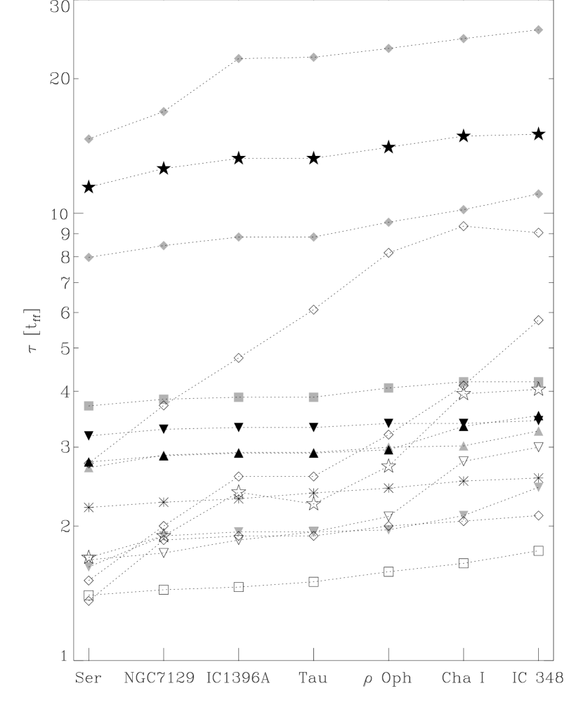
Figure 2: The time $\tau$ of the best correspondence between models and observations (in units of the global free-fall time $\tau_{\mathrm{ff}}$) for the seven investigated clusters. The symbols denote the parameters of the models: $\mathcal{M}=0.5$ (triangles), $\mathcal{M}=2$ (triangles down), $\mathcal{M}=3.2$ (squares), $\mathcal{M}=6$ (diamonds), $\mathcal{M}=10$ (stars); $1\leq k\leq 2$ (open symbols), $3\leq k\leq 4$ (grey symbols), $7\leq k\leq 8$ (filled symbols). The Gaussian collapse models are displayed as asterisks.

4 Discussion

4.1 The evolutionary sequence

Figure 1 shows the temporal evolution of the fractions of the different YSO classes for three selected models. The formation of the entire cluster takes place on varying timescales between about two and 25 global free-fall times. In the Gaussian collapse models and the turbulent models with small Mach numbers the formation tends to be faster, because self-gravity dominates the large scales. The numbers of Class 0 protostars show only a narrow peak, followed by a similar, but shifted peak of Class 1 objects. In the models with higher turbulence, the kinetic energy exceeds the gravitational one and the system is formally supported on global scales. Collapse only occurs locally in the shock compressed cloud clumps. The formation of Class 0 objects extends over a longer period (a few free-fall times) and in some cases there is a second burst of star formation, following an increase of the number of prestellar cores, at a later time as in model M6k2a or M10k2. This second peak is not considered for the comparison with the observations, though.

We count the numbers of objects in the particular classes and compare the relative numbers to the observational values from Table 1. We consider the entire observed population including more dispersed objects. Due to the use of periodic boundary conditions those are also included in the models.

The time $\tau$ of the best correspondence between observations and models is determined when the weighted root mean square of the differences

$$\sigma(t)=\sqrt{\frac{\frac{1}{2}\sum\limits_{i=0}^{2}{|n_{i}^{\mathrm{o}}-n_{i}^{\mathrm{m}}(t)|^{2}\omega_{i}}}{\sum\limits_{i=0}^{2}\omega_{i}}}$$ (1)

becomes a minimum. The relative number of young stars in Class $i$ (0, 1, 2) from observations is expressed as $n_{i}^{\rm o}$ and $n_{i}^{\rm m}$ denotes the relative number of YSOs in Class $i$ from the models. The factor $\omega_{i}$ is a weighting factor, introduced to account for the possible scatter due to small number statistics in both, the observations and the models. The weighting factor is set to $\omega_{i}=\sqrt{n_{i}^{\rm o}\cdot n_{i}^{\rm m}}$.

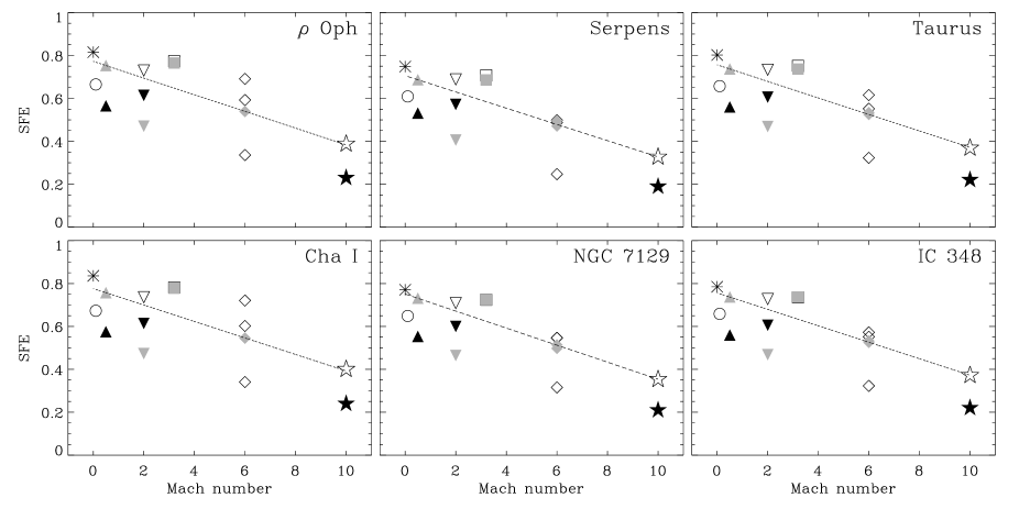
Figure 3: The star formation efficiency at time $\tau$ plotted versus the Mach number of the models. The symbols are the same as in Fig. 2, circles denote models with $\mathcal{M}=0.1$. The dotted lines show a linear fit to the data.

The time $\tau$ is shown in the lower panel of Fig. 1 and displayed for all models in Fig. 2. In general, Serpens is fitted worse than the other clusters. The mean minimal deviation of all models is $\langle\sigma_{\mathrm{min}}\rangle=0.006$ for $\rho$ Oph, Cha I, and IC 348, $\langle\sigma_{\mathrm{min}}\rangle=0.008$ for Taurus, $\langle\sigma_{\mathrm{min}}\rangle=0.009$ for IC 1396A, $\langle\sigma_{\mathrm{min}}\rangle=0.012$ for NGC 7129, and $\langle\sigma_{\mathrm{min}}\rangle=0.017$ for Serpens. In all cases $\sigma(t)$ has a clearly defined minimum. The scatter of $\tau$ is high. Its value varies from about 1.5 to 25 free-fall times for the different models, making it impossible to determine the actual ages of the clusters accurately. However, all models but one show the same sequence: $\tau$(Ser) $<\tau$(NGC 7129) $<\tau$(IC 1396A) $\approx\tau$(Tau) $<\tau$($\rho$ Oph) $<\tau$(Cha I) $<\tau$(IC 348). The only exception is model M6k2c, where $\tau$(IC 348) is slightly smaller than $\tau$(Cha I). In five models the age of IC 1396A is smaller than that of Taurus, in two models it is slightly larger, and in the other models the values are identical. Taking into account the second star-formation burst in the models M6k2a and M10k2 increases the ages of the older clusters, but it does not change the overall order. Thus, independent of the applied model, Serpens is the youngest cluster, NGC 7129 the second youngest cluster, Cha I and IC 348 are the most evolved clusters, while Taurus and IC 1396A are at roughly the same intermediate evolutionary stage. However, the relative numbers of Class 0 and 1 objects in NGC 7129 and IC 1396A may be overestimated due to possible observational biases introduced by the Spitzer Space Telescope, as discussed in Sect. 2.6. These clusters may thus appear younger relative to the other ones. The fact that $\sigma(t)$ always has one well-defined minimum and that all models produce the same evolutionary sequence independent of the initial conditions, supports a scenario of a single “burst” of uninterrupted, rapid star formation. This is in agreement with other theoretical and observational findings of star formation timescales and molecular cloud lifetimes (see e.g. Hartmann et al. hbb01 (2001); Ballesteros-Paredes & Hartmann bh04 (2005)). Several successive “bursts” of star formation within the cloud region are likely to alter the picture and make a determination of the age from the observed number ratios difficult.

4.2 Star formation efficiency

Figure 3 shows the star formation efficiency (the ratio of the mass accreted by the young stars to the total mass of the gas) at the time $\tau$ versus the Mach number of the models for six of the seven clusters. We find an inverse correlation of the SFE with the Mach number (false alarm probability $\leq 0.5\%$). This is consistent with the theoretical findings by Klessen et al. (KHM00 (2000)) and Heitsch et al. (HMK01 (2001)), and probably due to the fact that in high-Mach number turbulence less mass is available for collapse at the sonic scale (Vázquez-Semadeni et al. VBK03 (2003)). A linear fit is applied to the data and shown in Fig. 3. There is no correlation with the driving wave number. If we interpret the measured velocity dispersions in the clusters as the result of turbulence, we can estimate the SFEs at time $\tau$ for the particular Mach numbers from Fig. 3. In the case of $\rho$ Oph this requires to extrapolate the fit line beyond $\mathcal{M}=10$. The SFE is $\sim 0.27$ in $\rho$ Oph, $\sim 0.45$ in NGC 7129, $\sim 0.56$ in IC 348, and between 0.60 and 0.65 in Serpens, Taurus, and Cha I. (Lacking information on the velocity dispersion in IC 1396A, the corresponding SFE cannot be calculated.) These values are significantly higher than the measured SFEs, which are only around 0.1. (No information is available on the SFEs of IC 348 and NGC 7129, but we expect them to be in the range of the other clusters.) Only in the case of $\rho$ Oph the SFE of the models is in the range of the SFE measured. The main reasons for this discrepancy are probably the limitation of the gas reservoir and the neglect of outflows and feedback mechanisms as well as of magnetic fields in the simulations. Bipolar outflows limit the local SFE, because the protostellar jet will carry a certain fraction of the infalling material away, furthermore, its energy and momentum input will affect the the protostellar envelope and may partially prevent it from accreting onto the protostar (e.g. Adams & Fatuzzo af96 (1996)). The presence of magnetic fields would also retard the conversion of gas into stars (for current simulations see Heitsch et al. HMK01 (2001); Vázquez-Semadeni et al. vksb04 (2005); Li & Nakamura ln04 (2004)).

4.3 Prestellar cores

Table 2: The ratio of prestellar cores to the total number of YSOs at time $\tau$ for three models and the observations

Region	M2k4	M6k2a	M10k2	Observations
$\rho$ Oph	0.30	0.10	0.10	0.47
Serpens	0.79	0.06	0.74	0.39
Taurus	0.32	0.09	0.22	0.25
Cha I	0.18	0.11	0.82	$<0.39$

As an additional test, the numbers of prestellar cores are analysed as described in Sect. 3 for the three models shown in Fig. 1 and compared to the four star-forming regions, where information on the number of prestellar cores is available. The ratios of the number of prestellar cores to the total number of YSOs ($n_{\mathrm{psc}}/n_{*}$) at time $\tau$ are listed in Table 2 together with those values from the observations (calculated from Table 1). The observed ratio in Taurus are roughly represented by models M2k4 and M10k2, but for the other regions the models produce either a much higher or much lower ratio. We intended to check if $n_{\mathrm{psc}}^{\mathrm{o}}/n_{\mathrm{psc}}^{\mathrm{m}}$ allows us to draw conclusions about the number of prestellar cores that actually collapse and form stars. This seems not to be possible on the basis of the current analysis. In addition, defining a prestellar core is rather difficult, both, from an observational and a theoretical point of view. This adds another level of uncertainty to results based on prestellar core statistics.

5 Summary and conclusions

We analysed the temporal evolution of the fractions of YSO classes in different gravoturbulent models of star formation and compared it to observations of star-forming clusters. The observed ratios of Class 0, 1, 2/3 objects in $\rho$ Ophiuchi, Serpens, Taurus, Chamaeleon I, NGC 7129, IC 1396A, and IC 348 can be reproduced by the simulations, although the time when the observations are best represented varies depending on the model. Nevertheless, amongst the clusters with good observational sampling we always find the following evolutionary sequence of increasing age: Serpens, Taurus, $\rho$ Oph, Cha I, and IC 348.

We find an inverse correlation of the star formation efficiency with the Mach number. However, our models fail to reproduce the observed SFEs for most of the clusters. This is probably due to the lack of a sufficiently large gas reservoir in the simulations and the neglect of energy and momentum input from bipolar outflows and/or radiation from young stars. Only the SFE in $\rho$ Oph is reproduced. This region is characterised by very high turbulent Mach numbers. The fact that our simple gravoturbulent models without feedback are able to reproduce the right number ratios of YSOs for $\mathcal{M}\simeq 10$ suggests that protostellar feedback processes may not be important in shaping the density and velocity structure in star-forming regions with very strong turbulence and argues for driving mechanisms external to the cloud itself (see also the discussion in Ossenkopf & Mac Low Ossenkopf_MacLow02 (2002) and Mac Low & Klessen maclow_klessen04 (2004)).

The relative numbers of YSOs can reveal the evolutionary status of a star-forming cluster only with respect to other clusters, the absolute age is difficult to estimate. Better agreement between models and observations requires a better consideration of environmental conditions like protostellar outflows and magnetic fields in the simulations. A larger observational sample, achieved by complete censuses of more star-forming regions, is also desirable.

- (1) Adams, F. C., & Fatuzzo, M. 1996, ApJ, 464, 256
- (2) André, P., Ward-Thompson, D., & Barsony, M. 2000, in Protostars and Planets IV, ed. V. Mannings, A. P. Boss, & S. S. Russell (Tucson: University of Arizona Press), 59
- (3) Ballesteros-Paredes, J., & Hartmann, L. 2005, ApJ, submitted
- (4) Ballesteros-Paredes, J., Klessen, R. S., & Vázquez-Semadeni, E. 2003, ApJ, 592, 188
- (5) Bate, M. R., & Burkert, A. 1997, MNRAS, 288, 1060
- (6) Bate, M. R., Bonnell, I. A., & Price, N. M. 1995, MNRAS, 277, 362
- (7) Blitz, L. 1993, in Protostars and Planets III, eds. E. H. Levy & J. I. Lunine (Tucson: Univ. Arizona Press), 125
- (8) Bontemps, S., André, P., Kaas, A. A., et al. 2001, A&A, 372, 173
- (9) Cambrésy, L., Copet, E., Epchtein, N., et al. 1998, A&A, 338, 977
- (10) Elmegreen, B. G. 1993, ApJ, 419, L29
- (11) Froebrich, D. 2005, ApJS, 156, 169
- (12) Froebrich, D., Schmeja, S., Smith, M. D., & Klessen, R. S. 2005a, A&A, submitted
- (13) Froebrich, D., Scholz, A., Eislöffel, J., & Murphy, G. C. 2005b, A&A, 432, 575
- (14) Grosso, N., Montmerle, T., Bontemps, S., André, P., & Feigelson, E. D. 2000, A&A, 359, 113
- (15) Haikala, L. K., Harju, J., Mattila, K., & Toriseva, M. 2005, A&A, 431, 149
- (16) Hartmann, L. 2002, ApJ, 578, 914
- (17) Hartmann, L., Ballesteros-Paredes, J., & Bergin, E. A. 2001, ApJ, 562, 852
- (18) Heitsch, F., Mac Low, M.-M., & Klessen, R. S. 2001, ApJ, 547, 280
- (19) Hunter, J. H., & Fleck, R. C. 1982, ApJ, 256, 505
- (20) Hurt, R. L., & Barsony, M. 1996, ApJ, 460, L45
- (21) Jappsen, A.-K., & Klessen, R. S. 2004, A&A, 423, 1
- (22) Johnstone, D., Wilson, C. D., Moriarty-Schieven, G. et al. 2000, ApJ, 545, 327
- (23) Kaas, A. A., Olofsson, G., Bontemps, S., et al. 2004, A&A, 421, 623
- (24) Kamegai, K., Ikeda, M., Maezawa, H., et al. 2003, ApJ, 589, 378
- (25) Klein, R. I., Fisher, R., & McKee, C. F. 2004, Rev. Mex. Astron. Astrofís. (Ser. de Conf.), 22, 3
- (26) Klessen, R. S. 1997, MNRAS, 292, 11
- (27) Klessen, R. S. 2001, ApJ, 556, 837
- (28) Klessen, R. S., & Burkert, A. 2000, ApJS, 128, 287
- (29) Klessen, R. S., Heitsch, F., & Mac Low, M.-M., 2000, ApJ, 535, 887
- (30) Klessen, R. S., Ballesteros-Paredes, J., Vázquez-Semadeni, E., & Durán-Rojas, C. 2005, ApJ, 620,786
- (31) Lada, C. J. 1987, in Star Forming Regions, IAU Symp. 115, 1
- (32) Lada, C. J., & Lada, E. A. 2003, ARA&A, 41, 57
- (33) Larson, R. B. 2003, Rep. Prog. Phys., 66, 1651
- (34) Lee, C. W., & Myers, P. C. 1999, ApJS, 123, 233
- (35) Li, Z.-Y., & Nakamura, F. 2004, ApJ, 609, L83
- (36) Luhman, K. L., Stauffer, J. R., Muench, A. A., et al. 2003, ApJ, 593, 1093
- (37) Mac Low, M.-M., & Klessen, R. S. 2004, Rev. Mod. Phys., 76, 125
- (38) Megeath, S. T., Allen, L. E., Gutermuth, R. A., et al. 2004, ApJS, 154, 367
- (39) Men’shchikov, A. B., & Henning, T. 1997, A&A, 318, 879
- (40) Mizuno, A., Onishi, T., Yonekura, Y., et al. 1995, ApJ, 445, L161
- (41) Mizuno, A., Hayakawa, T., Tachihara, K., et al. 1999, PASJ, 51, 859
- (42) Monaghan, J. J. 1992, ARA&A, 30, 543
- (43) Motte, F., & André, P., & Neri, R. 1998, A&A, 336, 150
- (44) Muzerolle, J., Megeath, S. T., Gutermuth, R. A., et al. 2004, ApJS, 154, 379
- (45) Olmi, L., & Testi, L. 2002, A&A, 392, 1053
- (46) Onishi, T., Mizuno, A., Kawamura, A., Ogawa, H., & Fukui, Y. 1996, ApJ, 465, 815
- (47) Ossenkopf, V., & Mac Low, M.-M. 2002, A&A, 390, 307
- (48) Padoan, P. 1995, MNRAS, 277, 377
- (49) Padoan, P., & Nordlund, Å. 2002, ApJ, 576, 870
- (50) Persi, P., Marenzi, A. R., Gómez, M., & Olofsson, G. 2001, A&A, 376, 907
- (51) Preibisch, T. 2003, A&A, 410, 951
- (52) Preibisch, T., & Zinnecker, H. 2002, AJ, 123, 1613
- (53) Preibisch, T., & Zinnecker, H. 2004, A&A, 422, 1001
- (54) Reach, W. T., Rho, J., Young, E., et al. 2004, ApJS, 154, 385
- (55) Ridge, N. A., Wilson, T. L., Megeath, S. T., Allen, L. E., & Myers, P. C. 2003, AJ, 126, 286
- (56) Sasao, T. 1973, PASJ, 25, 1
- (57) Schmeja, S., & Klessen, R. S. 2004, A&A, 419, 405
- (58) Smith, M. D. 2000, Ir. Astron. J., 27, 25
- (59) Stanke, T., Smith, M. D., Gredel, R., & Khanzadyan, T. 2004, A&A, submitted
- (60) Testi, L., & Sargent, A. I. 1998, ApJ, 508, L91
- (61) Walter, F. M. 1986, ApJ, 306, 573
- (62) Vázquez-Semadeni, E., Ostriker, E. C., Passot, T., Gammie, C. & Stone, J. 2000, in Protostars and Planets IV, ed. V. Mannings, A. P. Boss, & S. S. Russell (Tucson: University of Arizona Press), 3
- (63) Vázquez-Semadeni, E., Ballesteros-Paredes, J., & Klessen, R. S. 2003, ApJ, 585, L131
- (64) Vázquez-Semadeni, E., Kim, J., Shadmehri, M., & Ballesteros-Paredes, J. 2005, ApJ, 618, 344
- (65) Williams, J. P., De Geus, E. J., & Blitz, L. 1994, ApJ, 428, 693
- (66) Young, C. H., Jørgensen, J. K., Shirley, Y. L., et al. 2004, ApJS, 154, 396