Inhomogeneous models of interacting dark matter and dark energy.

Abstract

We derive and analyze a class of spherically symmetric cosmological models whose source is an interactive mixture of inhomogeneous cold dark matter (DM) and a generic homogeneous dark energy (DE) fluid. If the DE fluid corresponds to a quintessense scalar field, the interaction term can be associated with a well motivated non–minimal coupling to the DM component. By constructing a suitable volume average of the DM component we obtain a Friedman evolution equation relating this average density with an average Hubble scalar, with the DE component playing the role of a repulsive and time-dependent $\Lambda$ term. Once we select an “equation of state” linking the energy density ($\mu$) and pressure ($p$) of the DE fluid, as well as a free function governing the radial dependence, the models become fully determinate and can be applied to known specific DE sources, such as quintessense scalar fields or tachyonic fluids. Considering the simple equation of state $p=(\gamma-1)\,\mu$ with $0\leq\gamma<2/3$, we show that the free parameters and boundary conditions can be selected for an adequate description of a local DM overdensity evolving in a suitable cosmic background that accurately fits current observational data. While a DE dominated scenario emerges in the asymptotic future, with total $\Omega$ and $q$ tending respectively to 1 and -1/2 for all cosmic observers, the effects of inhomogeneity and anisotropy yield different local behavior and evolution rates for these parameters in the local overdense region. We suggest that the models presented can be directly applied to explore the effects of various DE formalisms on local DM cosmological inhomogeneities.

I Introduction

Observational data on Type Ia supernovae strongly suggests that the universe is expanding at an accelerated ratenewuniv1 ; newuniv2 . This effect has lead to the widespread assumption that the inventary of cosmic matter–energy could contain, besides baryons, photons, neutrinos and cold dark matter (DM), an extra contribution generically known as “dark energy” (DE), whose kinematic effect could be equivalent to that of a fluid with negative pressure. While the large scale dynamics of the main cosmic sources (DE and DM) is more or less understood, their fundamental physical nature is still a matter for debate, thus various physical explanations have been suggested. Cold DM is usually conceived as a collisionless gas of supersymmetric particles (neutralinos), while DE can be modelled as a “cosmological constant”, quintessense scalar fields, tachyonic fluids, generalized forces, etcPadma1 ; Lima1 . The standard approach is mostly to consider a Friedman-Lemaître-Robertson-Walker (FLRW) metric, with linear pertubations, making also the simplest assumption that DE only interacts gravitationally with DM. However, there are still some unresolved issues, such as the so–called “coincidence problem”, concerning the odd apparent fact that the critical densities of DM and DE approximately coincide in our cosmic era amendola ; coinc1 . Aiming at a solution to this problem and bearing in mind our ignorance on the fundamental physics of DM and DE, various models have been proposed recently which include asorted forms of interaction between these sources Q-int1 ; Q-int2 ; Q-int3 ; Q-int4 ; Q-int5 .

It is customarily assumed that DE dominates large scale cosmic dynamics, so that DM inhomogeneities in galactic clusters and superclusters can be considered a local effect or can be treated by means of linear perturbations in a FLRW background. Thus, a reasonable generalization of existing models could be to assume inhomogeneous DM interacting with homogenous DE, so that large scale dynamics is governed by the latter. We propose in this paper a class of analytic models which provide a reasonable description of inhomogeneous DM interacting with a generic homogeneous DE source. The models are based on the spherically symmetric subcase of the Szafron–Szekeres exact solucions of Einstein’s field equations for a perfect fluid sourcekras . However, the underlying geometry of the models we present can be easily generalized to include non–spherical symmetries or even the case without any isometry, since, in general, Szafron–Szekeres solutions do not admit Killing vectors.

The prefect fluid in Szafron–Szekeres solutions in their original conception is characterized by a non–rotating geodesic 4-velocity field, so that in the comoving frame matter–energy density is inhomogeneous, while pressure depends only on cosmic time. As we show in section II, it is straightforward to re–interpret this fluid as a mixture of an inhomogeneous dust component plus a homogeneous fluid. Such mixture have been considered previously old2F1 ; old2F2 but in the context of mixtures of baryons and radiation. We consider in this paper only the type of models examined in old2F2 , by assuming the homogeneous fluid to describe a generic DE source, while the dust component corresponds to inhomogeneous DM, all of which is a reasonable assumption since the dynamical effects of quintessence mostly become dominant in very large scales, larger than the “homogeneity scale” (100–300 Mpc), while DM (galactic clusters and superclusters) is very inhomogeneous at scales of this magnitude and smaller. By conveniently rescaling the free parameters and calculating relevant physical and geometric quantities, we show in sections III, IV and V that the dynamical equation characterizing the models is analogous to a Friedman equation in which the average DM density evolves in the presence of a generic (still undetermined) time–dependent cosmological constant or “Lambda field”. By looking at the regularity conditions, singularities and asymptotic behavior along timelike and spacelike directions, we show in section VI that the DE and DM mixture components behave as needed for a reasonable cosmological model complying with observations: for all fundamental observers the DE source dominates over DM in the asymptotic timelike future, while boundary conditions determine how the local ratio of DE and DE changes along the rest frames of the fundamental observers. However, these frames (hypersurfaces of constant cosmic time) have zero curvature, hence the inhomogeneities in the models are more suitable for a study of large scale inhomogeneities than local structure formation, since even overdense regions homogeneize and isotropize towards an asymptotic DE dominated scenario. The main observational parameters are appropriately defined and calculated for an inhomogeneous and anisotropic spacetime in section VII.

In order to determine the time evolution of the sources, we need to assume a physical model, or “equation of state” for the generic DE source (the homogeneous fluid). Thus, we assume in section VIII a simple “gamma law” equation of state of the form $p=(\gamma-1)\,\mu$, where $p,\,\mu$ are the pressure and matter–energy density of the DE source. Such an equation of state leads to a DE homogeneous fluid evolving like a FLRW fluid with flat spacelike sections with a scaling law of the form $\mu\propto t^{-2}$, which is compatible with a scalar field with an exponential potential CJSF . Although this is a very simple type of DE source, it yields analytic forms for the DM density, observational parameters and allother relevant physical and geometric quantities.

The assumption of a gamma law equation of state fully determines the time dependence of all relevant quantities, but the free parameters governing spacial dependence are specified in section IX. Suitable boundary conditions can always be selected allowing for a description of a local DM overdense region in a DE dominated cosmic background that accurately complies with observational constraints on observational parameters: $\Omega$ for DM and for DE and the deceleration parameter $q$. We provide in this section a full graphical illustration of the interplay between “local” and “cosmic background” effects on these observational parameters: for example, anisotropy emerges in the local dependence of these quantities on the “off-center observation angle” $\psi$, while inhomogeneity leads to local conditions in the overdense region (DM dominates over DE and $q$ is positive) that are different from those of the cosmic background: DE dominates and $q<0$, as required by an “accelerated” universe whose large scale dynamics is dominated by a repulsive force associated with DE.

The issue of the interaction between DE and DM is dealt with in section X. We show that the individual momentum–energy tensors for DM and DE are not independently conserved, thus the models are incompatible with these components interacting only gravitationally. However, if we assume the DE fluid to be a scalar field quintessense type of source, then the models can accomodate various prescriptions for a DE–DM interaction, like those proposed in the literature Q-int1 ; Q-int2 ; Q-int3 ; Q-int4 ; Q-int5 . Finally, in section XI we present a discussion and summary of our results.

II Field equations for a class of inhomogeneous cosmologies.

We start with a spherically symmetric inhomogeneous spacetime, the spherical subcase of the Szafron–Szekeres solutions kras , which can be described by the Lemaitre–Tolman–Bondi (LTB) metric element

$$ds^{2}\ =\ -c^{2}\,dt^{2}+\frac{Y^{\prime}{}^{2}}{1-K}\,dr^{2}+Y^{2}\,\hbox{d}\Omega^{2},$$ (1)

with $K=K(r),\,\,Y=Y(t,r)$,    $\hbox{d}\Omega^{2}\equiv\hbox{d}\theta^{2}+\sin^{2}\theta\,\hbox{d}\varphi^{2}$ and a prime denotes derivative with respect to $r$. As matter source we consider a perfect fluid

$$T^{ab}\ =\ (e+p)\,u^{a}\,u^{b}+p\,g^{ab},$$ (2)

where $e$ and $p$ are the matter–energy density and total (effective) pressure. In a comoving representation with 4-velocity $u^{a}=\delta^{a}_{t}$ the field equations for (1) and (2) are

$$G^{r}_{r}=\kappa\,p = -\frac{K}{Y^{2}}-\frac{\dot{Y}^{2}}{Y^{2}}-\frac{2\ddot{Y}}{Y},$$ (3a)

$$G^{\theta}_{\theta}=G^{\phi}_{\phi}=\kappa\,p = -\frac{K^{\prime}}{2YY^{\prime}}-\frac{\dot{Y}\dot{Y}^{\prime}}{YY^{\prime}}-\frac{\ddot{Y}}{Y}-\frac{\ddot{Y}^{\prime}}{Y^{\prime}},$$ (3b)

$$-G^{t}_{t}=\kappa\,e = \frac{K}{Y^{2}}+\frac{\dot{Y}^{2}}{Y^{2}}-\frac{2Y^{\prime}\dot{Y}^{\prime}}{YY^{\prime}}-\frac{K^{\prime}}{YY^{\prime}},$$ (3c)

where $\kappa=8\pi G/c^{4}$ and a dot denotes derivative with respect to $ct$. Since the left hand sides of (3a) and (3b) are identical, we obtain the condition $G^{\theta}_{\theta}-G^{r}_{r}=0$, which yields

$$\frac{K}{Y^{2}}+\frac{\dot{Y}^{2}}{Y^{2}}+\frac{2\ddot{Y}}{Y}\ =\ -\kappa\,p(t).$$ (4)

an expected result since the comoving 4-velocity for (1) is a timelike geodesic vector and so is incompatible with spacelike gradients of $p$. If we keep $p(t)$ arbitrary, then we cannot obtain a simple integral of (4), but we can transform this condition into

$$\ddot{X}+\frac{3}{4}\,\kappa\,p\,X+\frac{3}{4}\,\frac{K}{X^{1/3}}\ =\ 0,$$ (5)

where $X=Y^{3/2}$, while matter–energy density in (3c) becomes

$$\kappa\,e\ =\ \frac{4}{3}\,\frac{\dot{X}\,\dot{X}^{\prime}}{X\,X^{\prime}}+\frac{K}{X^{4/3}}+\frac{3}{2}\,\frac{K^{\prime}}{X^{1/3}\,X^{\prime}}.$$ (6)

Hence, once we choose $p$ and $K$, we can find $X$ by integrating (5) and then $e$ becomes determined by means of (6). The solutions of Einstein’s field equations associated with (1), (5) and (6) are the spherically symmetric subcase of “class 1” Szekeres–Szafron solutions kras . However, for $K\neq 0$ there are no analytic solutions for the nonlinear equation (5), while finding a meaningful equation of state relating $p(t)$ and $e(t,r)$ is difficult.

III A mixture of dark matter and dark energy.

An alternative approach is to consider only the case $K=0$ (hypersurfaces $t=$ constant have zero curvature) and to assume that total matter–energy density decomposes as

$$e(t,r)\ =\rho(t,r)\,c^{2}+\mu(t),$$ (7)

so that we can re–interpret the momentum–energy tensor (2) as the mixture

$$T^{ab} = T^{ab}_{(1)}+T^{ab}_{(2)},\qquad\textrm{with:}$$

$$T^{ab}_{(1)} = \rho\,c^{2}\,u^{a}\,u^{b},\quad T^{ab}_{(2)}=(\mu+p)\,u^{a}\,u^{b}+p\,g^{ab}.$$

So, it is now more natural to choose $\mu$ and $p$, as matter–energy density and total pressure of a homogeneous fluid describing a specific physical system. Then, integrating the linear equation

$$\ddot{X}+\frac{3}{4}\,\kappa\,p\,X=0,$$ (9)

we can determine the metric and the rest–mass density of the inhomogeneous dust component

$$\kappa\,\rho\,c^{2}=\frac{\frac{4}{3}\,\dot{X}\dot{X}^{\prime}-\kappa\,\mu\,XX^{\prime}}{XX^{\prime}}.$$ (10)

This approach has been used in the past for modeling mixtures of baryons and radiation old2F1 ; old2F2 , but it can be equally useful to study the interaction between cold DM (the inhomogeneous dust: $T^{ab}_{(1)}$) and a generic (yet unspecified) type of DE (the homogeneous fluid $T^{ab}_{(2)}$ with negative pressure). Because of their construction, the two energy–momentum tensors are not separately conserved:   $T^{ab}_{(1)}{}_{;b}=-T^{ab}_{(2)}{}_{;b}\neq 0$, hence we must have a non–minimal coupling between DM and DE (see section X).

IV Determination of free parameters

Since (9) is a second order lineal partial differential equation, its solutions have the form

$$X\ =\ V(t)\,\alpha(r)+W(t)\,\beta(r),$$ (11)

where $\alpha(r),\,\beta(r)$ are the two “integration constants” that follow from the integration of (9) and the functions $V,\,W$ satisfy: $\ddot{V}/V=\ddot{W}/W=(3/4)\,\kappa\,p$. Since we can arbitrarily relabel the radial coordinate $r$, no loss of generality is involved if we relabel these functions as

$$V=R^{2/3},\qquad W=T\,R^{2/3},$$ (12a)

$$\qquad\alpha=r^{2/3},\qquad\beta=r^{2/3}\,f$$ (12b)

where $R(t),\,T(t)$ and $f(r)$ are arbitrary functions. Inserting (11) and (12) in (9) and demanding consistency with (4)–(6), we obtain the equations that (given a choice of $p=p(\mu)$) determine $R$ and $T$

$$\kappa\,p\ = \ -\frac{\dot{R}^{2}}{R^{2}}-\frac{2\ddot{R}}{R},$$ (13)

$$\kappa\,\mu\ = \ \frac{3\dot{R}^{2}}{R^{2}},$$ (14)

$$\dot{T}\ = \ c_{0}\,H_{0}\frac{R_{0}^{3}}{R^{3}},$$ (15)

where $c_{0}$ is a dimensionless constant, $R_{0}=R(t_{0})$ and $H_{0}$ can be identified with the Hubble timescale at $t_{0}$. The form of equations (13) and (14) is identical to the field equations of a FLRW spacetime with flat space sections, this suggest that we identify $\mu$ and $p$ with variables somehow associated with a FLRW background. Once we choose an “equation of state” $p=p(\mu)$ corresponding to a specific DE model for the homogeneous fluid (for example, a scalar field), we can find $R$ by integrating (13) and (14), and then $T$ by integrating (15).

An alternative approach follow by defining what would be a “Hubble factor” for an homogeneous fluid:

$$H\equiv\frac{\dot{R}}{R},$$ (16)

allowing us to combine equations (13) and (14) into

$$\dot{H}\ =\ -\frac{\kappa}{2}\,(\mu+p),\qquad\kappa\,\mu\ =\ 3\,H^{2},$$ (17)

so that, once the “equation of state” $p=p(\mu)$ is prescribed, we get $p=p(H)$. The functions $H$ and $R$ follow by integration of (17) and (16), which is equivalent to integrating (13) and (14).

Once we select $f$ (after solving (13)–(14) or (17)–(16)), the metric (1) and dust density (10), as well as any other geometric or physical variables, become fully determined. Under the parametrization given by (11) and (12), the metric (1) and DM mass–energy density (10) take the form

$$\hbox{d}s^{2}\ =\ -c^{2}\,\hbox{d}t^{2}+R^{2}\,\left[\,\frac{(1+F\,T)^{2}}{(1+f\,T)^{2/3}}\,\hbox{d}r^{2}+r^{2}\,(1+f\,T)^{4/3}\,\hbox{d}\Omega^{2}\right],$$ (18)

$$\kappa\,\rho\,c^{2}\ = \ \frac{4\,(3\,T\,H+\dot{T})\,f\,F+6\,H\,(f+F)}{3\,(1+f\,T)\,(1+F\,T)}\,\dot{T}$$ (19)

$$= \frac{2\,c_{0}\,H_{0}\,R_{0}^{3}}{3\,R^{6}}\,\frac{\frac{d}{dt}[\,(2\,T\,f\,F+f+F)\,R^{3}\,]}{(1+f\,T)\,(1+F\,T)}$$

where we used (15) and

$$F\equiv f+\frac{2}{3}\,r\,f\,^{\prime}.$$ (20)

Other important quantities are the expansion kinematic scalar $\Theta=u^{a}\,_{;a}$ and the traceles symmetric shear tensor $\sigma_{ab}=u_{[a;b]}-(\Theta/3)\,h_{ab}$

$$\Theta\ = \ 3\,H+{\cal{Z}}\,\dot{T},$$ (21)

$$\sigma^{a}\,_{b}\ = \ \textrm{\bf{diag}}\,[\,0,\,-2\Sigma,\,\Sigma,\,\Sigma],$$ (22)

where

$${\cal{Z}}\ = \ \frac{f+F+2\,f\,F\,T}{(1+f\,T)\,(1+F\,T)},$$ (23)

$$\Sigma\ = \ \frac{(F-f)\,\dot{T}}{(1+f\,T)\,(1+F\,T)}.$$ (24)

The metric (18) looks like a FLRW line element modified by the terms containing $T,\,F$ and $f$. In fact, all $r$–dependent variables derived above reduce to their FLRW forms: $\rho=\sigma=0,\,\Theta/3=H$,  if these “pertubations” vanish, i.e if either $T=0$ or $f=f^{\prime}=0$. This homogeneous subcase is a FLRW spacetime whose source is the DE perfect fluid with matter–energy density and pressure given by $\mu$ and $p$. In a sense, if $f\,T\ll 1$ and $F\,T\ll 1$ the models would correspond formally to specific exact perturbations of FLRW cosmologies.

V A time dependent $\Lambda$–field

It is possible to interpret the homogeneous DE fluid as a time dependent “cosmological constant”. For this purpose we recall that (1) and (18) are particular cases of the general spherically symmetric spacetime

$$ds^{2}=-A^{2}(t,r)\,c^{2}dt^{2}+B^{2}(t,r)\,dr^{2}+Y^{2}(t,r)\,d\,\Omega^{2}.$$ (25)

If the source of (25) is also a perfect fluid like (2), we can define a “mass function” $M$

$$M=\frac{Y}{2}\,\left[1+\frac{\dot{Y}^{2}}{A^{2}}-\frac{Y^{\prime}{}^{2}}{B^{2}}\right],$$ (26)

satisfying

$$2\,\dot{M} = -\kappa\,p\,Y^{2}\dot{Y},$$ (27a)

$$2\,M^{\prime} = \kappa\,e\,Y^{2}\,Y^{\prime}.$$ (27b)

For spherical symmetry and in the appropriate limit, $M$ coincides with the ADM and Hawking masses. In particular, for the metric (1) in the form of (18) and matter energy density (7), $M$ can be found by integrating (27b)

$$2\,M=\kappa\int{(\rho c^{2}+\mu)Y^{2}Y^{\prime}\,dr}=2\,{\cal{M}}+\frac{\kappa\,\mu}{3}\,Y^{3},$$ (28)

with

$$2\,{\cal{M}}\ \equiv \ \kappa\,c^{2}\int{\rho Y^{2}Y^{\prime}\,dr}$$ (29)

$$= \frac{4}{9}\,R^{3}\,r^{3}f\,\dot{T}\,[\,3\,H\,(1+f\,T)+f\,\dot{T}\,],$$

where we have assumed $M(t,0)=0$ and used $Y$ and $Y^{\prime}$ given by (18), as well as (19) and (20) expressed as $F=2(r^{3/2}f)^{\prime}/(3\sqrt{r})$. Equation (26) yields then the Friedman–type evolution equation

$$\dot{Y}^{2}=\frac{2\,M}{Y}=\frac{2{\cal{M}}}{Y}+\frac{\kappa\,\mu}{3}\,Y^{2},$$ (30)

in which ${\cal{M}}$ and $\kappa\mu$ respectively play the roles of “efective mass” of the inhomogeneous dust (DM) and a homogeneous time dependent $\Lambda$ term (DE). The mass function $M$ can be related to a volume average of the total energy density by

$$\kappa\,\langle\rho c^{2}+\mu\rangle = \frac{\kappa\int{(\rho c^{2}+\mu)Y^{2}Y^{\prime}\,dr}}{\int{Y^{2}Y^{\prime}\,dr}}=\frac{6\,M}{Y^{3}}$$ (31)

$$= \frac{6\,{\cal{M}}}{Y^{3}}+\kappa\mu.$$

Hence, we can identify the averaged DM and DE densities

$$\kappa\,c^{2}\langle\rho\rangle = \frac{6\,{\cal{M}}}{Y^{3}}\ =\ \frac{4[\,3\,H\,(1+f\,T)+f\,\dot{T}\,]}{3\,(1+f\,T)^{2}}\,f\,\dot{T},$$

$$\kappa\langle\mu\rangle = \kappa\,\mu\ =\ 3\,H^{2},$$ (32b)

so that (30) can be related to (32) and expressed as

$$\frac{\dot{Y}^{2}}{Y^{2}}\ =\ \frac{\kappa}{3}\,\langle\rho\rangle\,c^{2}+\frac{\kappa}{3}\,\langle\mu\rangle,$$ (33)

which looks like a FLRW Friedmann equation for a source made up with dust plus a time dependent $\Lambda$ term, $\mu$, but both given in terms of their averaged densities (32). In this context, we can identify the relative velocity $\dot{Y}/Y$ as a sort of averaged Hubble factor.

VI Regularity conditions and asymptotics

For a spherically symmetric spacetime (18) characterized by (7)–(15), the functions $R$,  $T$, $f$ and $F$ must comply with

$$R\ >\ 0,$$ (34a)

$$1+f\,T\ >\ 0,$$ (34b)

$$1+F\,T\ >\ 0.$$ (34c)

Hence, from (19), the condition $\rho\geq 0$ becomes

$$[\,4\,(\,3\,T\,H+\dot{T})\,f\,F+6\,H\,(f+F)]\,\dot{T}\ \geq\ 0$$ (35)

so that we can identify $t$ such that $R=0$ with a simultaneous big–bang singularity associated with $\mu\to\infty$ (with $\rho$ finite) and two singularities for which $\rho\to\infty$ (with $\mu$ finite)

$$1+f\,T\ =\ 0,$$ (36a)

$$1+F\,T\ =\ 0,$$ (36b)

which, in general, will be marked as non–simultaneous surfaces in the $(t,r)$ coordinate plane. Notice that (36a) is a non–simultaneous big–bang, or a central singularity ($\Rightarrow\,Y=0$), while (36b) is a shell crossing singularity ($\Rightarrow\,Y^{\prime}=0$), both analogous to singularities in Lemaître–Tolman–Bondi and Szekeres dust solutions singSZ . Hence, we will demand that

$$Y^{\prime}>0\,\,\textrm{holds for all}\,\,(t,r)\,\,\textrm{complying with}\,\,Y>0,$$ (37)

or equivalently, that (36b) does not occur in the coordinate range that complies with (34b). As shown in figure 1, condition (37) can be be satisfied by suitable choices of free parameters.

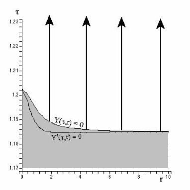
Figure 1: The plot depicts the coordinate representation of the non–simultaneous “big bang” singularity $Y(\tau,r)=0$ as a “surface” in the $(\tau,r)$ plane, with the dimensionless time $\tau$ defined by (55a) and other free parameters given by (54), (55) and (60). The domain of regularity, $Y>0$, is shown with worldlines of fundamental observers (arrows). Notice that the surface $Y^{\prime}=0$ occurs in the region with negative $Y$ (gray shading).

A usual regularity demand in spherically symmetric spacetimes is the existence of a symmetry center, characterized by the regular vanishing of the surface area of the orbits of SO(3). This condition defines the worldline of a privileged “central” observer for whom the universe appears isotropic. From (18) and marking this worldline by $r=0$, we must have for all $t$

$$Y_{(c)}=\dot{Y}_{(c)}=0$$ (38)

where $Y_{(c)}=Y(t,0)$. We shall use henceforth the subindex _(c) to denote evaluation at $r=0$. Since spacial gradients of $\rho,\,\Theta,\,\Sigma$ must vanish at the center, equations (19) and (20)–(24) imply that $f_{(c)}$ must be bounded and $f^{\prime}_{(c)}=0$, so that $F_{(c)}=f_{(c)}$. The central values of these quantities are then given by

$$\kappa\,\rho_{(c)}\,c^{2} = \frac{4}{3}\,f_{(c)}\,\frac{3\,H\,[1+f_{(c)}\,T]+f_{(c)}\,\dot{T}}{[1+f_{(c)}\,T]^{2}}\,\dot{T},$$ (39a)

$$\frac{\Theta_{(c)}}{3} = \left[\frac{\dot{Y}}{Y}\right]_{(c)}=H+\frac{2\,f_{(c)}\,\dot{T}}{3\,[1+f_{(c)}\,T]},$$ (39b)

$$\Sigma_{(c)} = 0\qquad\Rightarrow\quad[\sigma^{a}\,_{b}]_{(c)}=0$$ (39c)

where $f_{(c)}>0$ and $f(r)$ for $r>0$ must be selected so that $\rho$ decreases with increasing $r$.

In order to get an idea of the behavior of the models in the asymptotic limit $t\to\infty$, we may assume as $t\to\infty$ an asymptotic power law scaling $R\to t^{k}$ for $k>0$. From (15), we have $\dot{T}\to 0$ in this limit, but $T$ tends to a finite asymptotic value ($T\to T^{*}$) only for $k>1/3$. From (14), (15) we have

$$\mu\ \to\ \frac{3\,k^{2}}{t^{2}},\qquad p\ \to\ \frac{k\,(2-3k)}{t^{2}}$$ (40)

while, assuming $f$ and $F$ everywhere finite, we have from (14) and (19) the ratio

$$\frac{\rho\,c^{2}}{\mu} \to \ 0,\quad\textrm{for}\quad k>1/3,$$ (41a)

$$\frac{\rho\,c^{2}}{\mu} \to \ \textrm{const},\quad\textrm{for}\quad 0<k<1/3.$$ (41b)

Therefore, the homogeneous DE fluid dominates asymptotically over the DM component even if $p>0$ (or equivalently $k<2/3$), while values of $k$ associated with negative $p$ always yield the asymptotic ratio (41a). It is not difficult to verify that the same asymptotic behavior occurs if $R$ follows exponential or logarithmic asymptotic scalings, $R\to\exp(k\,t)$ or $R\to\ln\,t$. Thus, it is generically possible to have an asymptotically DE dominated asymptotic scenario for all fundamental observers, which is an important property of the models under consideration. As long as $R$ scales asymptotically faster than $R\to t^{2/3}$ and  $f,\,F$, are finite everywhere, we have $p<0$ together with

$$\frac{\Theta}{3}\to H,\qquad\Sigma\to 0,\qquad\textrm{as}\quad t\to\infty,$$ (42)

so that, regardless of the choice of $f$ (spacial dependence), the models homogenize and isotropize for all fundamental observers ($R$ constant) as $t\to\infty$, implying that all fundamental observers detect in this asymptotic limit local conditions that are very close to those of a FLRW cosmology characterized by a DE source with $\mu$ and $p$.

It is also interesting to examine the behavior of the models as $r\to\infty$ along hypersurfaces of constant $t$, the rest frames of fundamental comoving observers. It is important to notice that the radial coordinate, $r$, merely labels the fundamental comoving observers, so it has no invariant meaning and can be though of as a dimensionless ratio, such as $r=\ell/\ell_{0}$, where $\ell_{0}$ is the present value of an arbitrary length scale (for example, the scale of homogeneity $\ell_{0}\sim 100-300$ Mpc). Thus, we can consider “local” scales ($\ell\ll\ell_{0}$) as marked by $r\ll 1$, so that asymptotic “cosmic” scales correspond to $r\gg 1$, while the “transition” from local to cosmic scales is roughly given by $r\sim 1$.

Since $f$ is the free function that governs the dependence on $r$, the variation of all quantities in the radial direction is tied to specific choices of this free function. In particular $f$ should be selected so that $\rho$ decays as $r$ increases. Also, the spacial dependence of ${\cal{M}}$, the “effective mass” of DM defined by (29), is governed by the term $r^{3}f$, thus it is also convenient to demand that $f\geq 0$ and that $r^{3}f$ must be a monotonously increasing function. Still, considering all these restrictions, it is possible to select $f$ so that

$$f\to 0,\quad F\to 0,\qquad\textrm{as}\quad r\to\infty,$$ (43)

which is a sufficient condition for

$$\frac{1}{3}\,\Theta|{}_{r=\infty}\to H,\qquad\rho|{}_{r=\infty}\to 0,\qquad\Sigma|{}_{r=\infty}\to 0.$$ (44)

Thus, since $\mu$ is independent of $r$, these limits imply that local conditions for fundamental observers with large $r$ are similar those of fundamental observers of a FLRW cosmology whose source is a fluid with $\mu$ and $p$ (that is, a “pure” DE fluid). Another possibility is furnished by the choice:

$$f\to f^{*},\quad F\to f^{*},\qquad\textrm{as}\quad r\to\infty,$$ (45)

where $f^{*}<f_{(c)}$ is a positive constant. This yields

$$\kappa\,\rho|{}_{r=\infty}\,c^{2} = \frac{4}{3}\,f^{*}\,\frac{3\,H\,[1+f^{*}\,T]+f^{*}\,\dot{T}}{[1+f^{*}\,T]^{2}}\,\dot{T},$$ (46a)

$$\frac{1}{3}\,\Theta|{}_{r=\infty} = \left[\frac{\dot{Y}}{Y}\right]_{r=\infty}=H+\frac{2\,f^{*}\,\dot{T}}{3\,[1+f^{*}\,T]},$$ (46b)

$$\Sigma|{}_{r=\infty} = 0\qquad\Rightarrow\quad[\sigma^{a}\,_{b}]_{r=\infty}=0.$$ (46c)

The preference of one of these choices of asymptotic behavior along the rest frames depends on the problem one is interested to study: if we want to examine a large scale (supercluster scale or larger) spherical inhomogeneity whose evolution requires that we somehow “plug in” the effects of a cosmological background, then the choice (45) may be preferable, while the choice (43) may be preferable for a relatively small scale and/or large density contrast description of an homogeneity (cluster of galaxies) that ignores cosmic effects (see figure 3).

It is also possible to perform a smooth matching, for a comoving radius $r_{b}$, of a region $0\leq r\leq r_{b}$ of the DM and DE mixture to a spatially flat FLRW spacetime characterized by $\mu$ and $p$, occupying $r>r_{b}$. Necessary and sufficient conditions follow if $f_{(b)}=F_{(b)}=0$, where _(b) denotes evaluation at $r=r_{b}$, so that $\rho_{(b)}=\Sigma_{(b)}=0$ and $\Theta_{(b)}/3=H$ hold for the FLRW region. However, such a matching also requires the mass function $M$ in (26) to be continuous (at least $C^{0}$) at $r=r_{b}$, which from (28) implies ${\cal{M}}_{(b)}=0$, but ${\cal{M}}$ is a volume integral of $\rho$. Therefore, if this integral must vanish at $r=r_{b}$ for all $t$, the dust density $\rho$ in the integrand must necessarily be negative in a finite domain of the mixture region $0\leq r\leq r_{b}$. Hence, we will not consider this type of matching any further.

VII Observational parameters

The quantity $H$ in (16) is the Hubble expansion factor associated with a FLRW geometry, for the inhomogeneous metric (18) the proper generalization of this parameter is given by ellis ; HMM

$${\cal{H}}\ =\ \frac{\Theta}{3}+\sigma_{ab}\,n^{a}n^{b},$$ (47)

where the vector $n^{a}$ complies with $n_{a}n^{a}=1,\,u_{a}n^{a}=0$. For a spherically symmetric spacetime, it is necessary to evaluate $n^{a}$ for general comoving observers located in an “off–center” position in the spherical coordinates $(r,\theta,\phi)$ centered at $r=0$. For the metric (18) equation (47) becomes in general

$${\cal{H}}\ = \ H+{\cal{F}}\,\dot{T}$$

$${\cal{F}}\ = \ \frac{2\,[f\,(1+F\,T)+\frac{3}{2}\,(F-f)\,\cos^{2}\psi]}{3\,(1+f\,T)\,(1+F\,T)},$$ (48)

where $\psi$ is “observation angle” between the direction of a light ray and the “radial” direction for a fundamental observer located in $(r,\theta,\varphi)$ HMM . Therefore, the exact local values of the observational parameters $\Omega$ for DE and DM are

$$\Omega_{\textrm{\tiny{DE}}}\ = \ \frac{\kappa\,\mu}{3\,{\cal{H}}^{2}}=\frac{H^{2}}{\left[H+{\cal{F}}\,\dot{T}\right]^{2}},$$ (49)

$$\Omega_{\textrm{\tiny{DM}}}\ = \ \frac{\kappa\,\rho\,c^{2}}{3\,{\cal{H}}^{2}}=\frac{\kappa\,\rho\,c^{2}}{3\,\left[H+{\cal{F}}\,\dot{T}\right]^{2}}=\frac{\rho\,c^{2}}{\mu}\,\Omega_{\textrm{\tiny{DE}}},$$ (50)

while the acceleration parameter is ellis

$$q\ =\ \frac{6\Sigma^{2}}{{\cal{H}}^{2}}+\frac{\Omega_{\textrm{\tiny{DE}}}+\Omega_{\textrm{\tiny{DM}}}}{2}\,\left[1+\frac{3\,p/\mu}{1+\rho c^{2}/\mu}\right],$$ (51)

where $\Sigma$ is given by (24).

If we consider the flow of cosmic DM with density $\rho$ at the length scale of the observable universe ($\sim 3000\,h$ Mpc), then present day values of shear and DM density gradients in comparable scales are severely restricted by the near isotropy of the CMB CMBinh

$$\left[\frac{|\sigma_{ab}\,\sigma^{ab}|^{1/2}}{\Theta}\right]_{0}\ =\ \left[\frac{\sqrt{6}\,|\Sigma|}{\Theta}\right]_{0}\ \lesssim\ 10^{-5},$$ (52)

$$\left[\frac{h_{a}^{b}\,\rho_{,b}}{\rho}\right]_{0}\ =\ \left[\frac{\rho\,^{\prime}}{\rho}\right]_{0}\ \lesssim\ 10^{-5}.$$ (53)

Hence the large scale spacial dependence of the observational parameters (47), (49), (50) and (51) must also be restricted by these bounds. However, these restrictions can be strongly relaxed, at a local level, if we examine the spacial variation of local values of DM density and observational parameters in scales smaller than the homogeneity scale $\sim 100-300$ Mpc. As mentioned in the previous section, scale considerations influence the choice of boundary conditions (43) or (45).

Figure 2: Figure (a) illustrates how the present DM density profile, $\rho/\mu$, exhibits an increasingly large inhomogeneous contrast as $\delta$ ranges from $\delta=670$ (maximal contrast) to $\delta=0.1$ (minimal contrast). We have used (54) and (55) and the free parameters $f,\,\gamma,\,f^{*},\,T^{*}$ are those given by (60) and (64). Notice how for all $\delta$, we have $\mu>\rho c^{2}$ in the cosmic background region, with all curves tending as $r\to\infty$ to the cosmic ratio $\Omega_{\textrm{\tiny{DM}}}/\Omega_{\textrm{\tiny{DE}}}\approx 0.56$. Figure (b) displays the plot of a measure of density contrast between the center and $r=\infty$, given by $\Delta\rho/\rho=\rho(\tau_{0},0)/\rho(\tau_{0},\infty)-1$, as a function of $\log_{10}\delta$. Notice how the contrast grows proportionally to $\delta$, well beyond the linear perturbation regime.

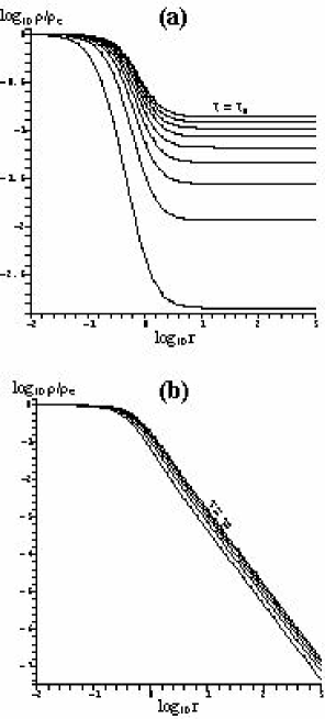
Figure 3: The panels depict the logarithmic profile of $\rho/\rho_{(c)}$, with $\rho_{(c)}=\rho(\tau,0)$ for a sequence of values of constant $\tau$, up to the present $\tau=\tau_{0}$. The free parameters $\gamma,\,\delta,\,T^{*}$ are those given by (64). In panel (a) we selected $f^{*}=100$, hence $\rho/\rho_{c}$ tends to the nonzero asymptotic cosmic DM density given by (46a). We see a power law decay of DM density only in the transition ($r\sim 1$) from the central overdensity region to the cosmic background. In panel (b) we selected $f^{*}=0$, thus the curves closely resemble isothermal profiles, in which $\rho$ decays to zero approximately as $r^{-2}$. This is not surprising since ${\cal{M}}\to r$ asymtotically with the choice (60).

VIII A simple example: the “gamma law”.

In order to illustrate how to work out the expressions we have derived and how to calculate relevant quantities of the models, we consider now the simple case of a homogeneous DE fluid satisfying a simple equation of state known as the “gamma–law”

$$p\ =\ (\gamma-1)\,\mu,$$ (54)

where $\gamma$ is a constant. The dust plus homogeneous fluid mixtures that we are studying were examined previously old2F1 , assuming (among other choices) this equation of state, but placing especial emphasis in a dust and radiation ($\gamma=4/3$) mixture. Since our emphasis is now on modelling DE sources, we will assume $0<\gamma<2/3$, so that $-1<p/\mu<-1/3$. In this case we have from (13), (15), (14), (16) and (17)

$$a \equiv \frac{R}{R_{0}}=\tau^{2/3\gamma},\qquad\tau\ =\ \frac{3}{2}\,\gamma\,h\,H_{0}\,t,$$ (55a)

$$\kappa\,\mu = 3\,H^{2}\ =\ \frac{3\,(hH_{0})^{2}}{\tau^{2}},$$ (55b)

$$T = T^{*}-\frac{\gamma_{1}}{\tau^{1/\gamma_{1}}},\qquad\gamma_{1}\ =\ \frac{\gamma}{2-\gamma}$$ (55c)

where $H_{0}=100\,\textrm{km}/(\textrm{sec\,Mpc})$, $h=0.7$ and $T^{*}$ is a dimensionless constant denoting the asymptotic value of $T$ (we have then in (15) the choice $c_{0}=\frac{3}{2}\,\gamma\,h$).

Notice that the assumptions (55) have been obtained from the FLRW equations (13) and (14) and yield a power law form for the function $a$ (equivalent to the FLRW scale factor). Therefore, following CJSF , this form of the homogeneous DE fluid is equivalent to a scalar field with an exponential potential following the so–called “scaling law”.

The density of the dust component and the generalized Hubble factor are found by inserting (55) into (19) and (48)

$$\kappa\rho c^{2}\ = \ \frac{3\,\gamma^{2}\,H_{0}^{2}}{\tau^{2}}\,\frac{\left[2\,T^{*}\,f\,F+(1/\gamma)\,(f+F)\right]\,\tau^{1/\gamma_{1}}+\gamma_{2}\,f\,F}{\left[\,(1+f\,T^{*})\,\tau^{1/\gamma_{1}}-\gamma_{1}\,f\,\right]\,\left[\,(1+F\,T^{*})\,\tau^{1/\gamma_{1}}-\gamma_{1}\,F\,\right]},\qquad\gamma_{2}\ =\ \frac{2-3\,\gamma}{2-\gamma},$$ (56)

$${\cal{H}}\ = \ \frac{h\,H_{0}}{\tau}\,\left\{1+\gamma\,\frac{\left[\,(1+F\,T^{*})\,\tau^{1/\gamma_{1}}-\gamma_{1}\,F\,\right]f+\frac{3}{2}\,(F-f)\,\tau^{1/\gamma_{1}}\,\cos^{2}\psi}{\left[\,(1+f\,T^{*})\,\tau^{1/\gamma_{1}}-\gamma_{1}\,f\,\right]\,\left[\,(1+F\,T^{*})\,\tau^{1/\gamma_{1}}-\gamma_{1}\,F\,\right]}\right\}.$$ (57)

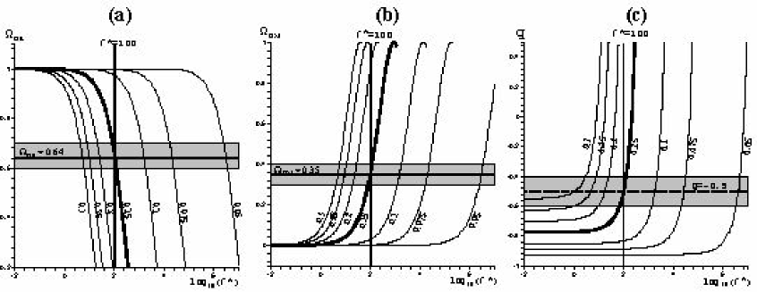
Figure 4: The asymptotic value of $f$ in (60) is given by $f^{*}$. Assuming $T^{*}=0$ and an arbitrary $\delta$, we can find a suitable value for $f^{*}$, for any given $\gamma$ in (54), by demanding that the observational parameters $\Omega_{\textrm{\tiny{DE}}},\,\Omega_{\textrm{\tiny{DM}}},\,q$ (panels (a),(b) and (c)) have appropriate “present” cosmological values in the ranges (63) as $r\to\infty$ for $\tau=\tau_{0}$ (gray stripes). Each curve is marked by a given value of $\gamma$. Notice that for $\gamma=0.15$, the choice $f^{*}\approx 100$ yields $\Omega_{\textrm{\tiny{DE}}}=0.64,\,\Omega_{\textrm{\tiny{DM}}}=0.35,\,q=-1/2$, which are reasonably close to currently accepted observational data. For $\gamma$ closer to $0$ (cosmological constant), we would have to select larger values for $f^{*}$, while larger $\gamma$ close to $0.3$ correspond to $f^{*}\sim 1$.

From (55), we see that $R$ scales as $t^{k}$, so that $k>1/3$ for $\gamma<2$, hence for the $\gamma$ values that we are interested we should obtain the ratio $\rho c^{2}/\mu$ given by (41a). Using (55b) and (56) and assuming an arbitrary but finite $f$ and $F$, we obtain in the limit $\tau\gg 1$

$$\frac{\rho\,c^{2}}{\mu} \to \frac{2\,T^{*}\,f\,F+(1/\gamma)\,(f+F)}{(1+f\,T^{*})\,(1+F\,T^{*})}\ \frac{3\,\gamma^{2}}{\tau^{1/\gamma_{1}}}\ \to\ 0,$$ (58)

$${\cal{H}} \to \frac{h\,H_{0}}{\tau}=H$$ (59)

indicating that for all cosmic observers the mixture homogenizes and isotropizes as the homogeneous DE fluid dominates asymptotically over the cold DM component.

IX Numerical exploration.

Having found $T,\,H$ and $a=R/R_{0}$ for the particular case of a gamma law (54), we only need to select the function $f=f(r)$ in order to render the models fully determinate. A convenient form for $f$ is

$$f\ =\ f^{*}+\frac{\delta}{1+r^{2}},$$ (60)

so that both type of asymptotic boundary conditions, (43)–(44) or (45)–(46), can be accomodated by selecting $f^{*}$ to be zero or nonzero. Notice also that asymptotically as $r\to\infty$, we have:  ${\cal{M}}\to r$ if $f^{*}=0$ and ${\cal{M}}\to r^{3}$ if $f^{*}>0$.

Considering (34), the regular evolution range for the models is the coordinate range $(\tau,r)$ where (37) holds with $a,\,H,\,T$ given by (54), (55) and $f,\,F$ given by (20) and (60). Thus, assuming as the initial “big–bang” the coordinate surface (36a) marking $Y=0$, we can take the big bang time as the value $\tau=\tau_{\textrm{bb}}$ at this surface corresponding to $r\to\infty$ (see figure 1), that is:

$$\tau_{\textrm{bb}}^{1/\gamma_{1}}=\frac{\gamma_{1}\,(f^{*}+\delta)}{1+(f^{*}+\delta)\,T^{*}}$$ (61)

Thus, considering the “age of the universe” roughly as $\Delta t_{0}\approx 14$ Gys and $h\approx 0.7$, the present cosmic era corresponds to

$$\tau_{0}=\tau_{\textrm{bb}}+\frac{3}{2}\gamma\,h\,H_{0}\,\Delta t_{0}\approx\tau_{\textrm{bb}}+3.17\,\gamma$$ (62)

As shown in figure 1, the big bang surface (36a) is not simultaneous, thus for any hypersurface $\tau=$ constant, the regions near the center at $r=0$ will be “younger” than those asymptotically far at large values of $r$.

The parameter $\delta=f_{(c)}-f^{*}>0$ in (60) provides the a measure of inhomogeneity contrast, or “spacial” variation of all quantities along the rest frames ($t=$ constant) between the symmetry center $r=0$ and $r\to\infty$. Thus, a sufficiently large/small value of $\delta$ makes the values at $r=0$ and $r\to\infty$ sufficiently close/far to each other, thus indicating small/large “contrast” or degree of inhomogeneity. We test the effect of $\delta$ along the present day hypersurface $\tau=\tau_{0}$ by plotting in figure 2a the spacial profiles of $\rho c^{2}/\mu$ for a sequence of $\delta$ values, while figure 2b depicts the density contrast between the overdensity at center and the cosmological background, as a function of $\log_{10}\delta$.

The effect of selecting $f^{*}$ zero or nonzero is shown in figures 3a and 3b, by means of a comparison between the resulting DM density profiles that follow by evaluating (56) and (60) along a sequence of hypersurfaces of constant $\tau$ (up to $\tau_{0}$). The asymptotic condition (43) ($f^{*}=0$) yields an approximately $r^{-2}$ power law decay of $\rho$ that resembles a standard isothermal profile, all of which is consistent with (44) and with the fact that the form of $f$ in (60), with $f^{*}=0$, leads to ${\cal{M}}\to r$, the same asymptotic behavior of the standard “isothermal sphere”. On the other hand, the choice (45) ($f^{*}>0$) leads also to a power law decay of $\rho$, but towards a cosmological background with asymptotic density given by (46).

The appropriate numerical value for the asymptotic constant, $f^{*}$, can be found by demanding that the cosmological observational parameters $\Omega_{\textrm{\tiny{DE}}},\,\Omega_{\textrm{\tiny{DM}}},\,q$, evaluated in the cosmic background ($r\to\infty$) at the present era ($\tau=\tau_{0}$), take (for a given $\gamma$) reasonably close values to those currently accepted from observational data. Since (57) with $T^{*}=0$ and $f$ given by (60), evaluated at $\tau=\tau_{0}$ and $r\to\infty$, is independent of $\delta$ and $\psi$, we can plot $\Omega_{\textrm{\tiny{DE}}},\,\Omega_{\textrm{\tiny{DM}}},\,q$ as functions of $f^{*}$ and $\gamma$. As figures 4a, 4b and 4c illustrate, the desired value of $f^{*}$ for any given $\gamma$ can be selected so that the forms (49), (50) and (51) at $\tau=\tau_{0}$ and $r\to\infty$ yield:

$$0.6 < \Omega_{\textrm{\tiny{DE}}}<0.7,$$ (63a)

$$0.3 < \Omega_{\textrm{\tiny{DM}}}<0.4,$$ (63b)

$$-0.5 < q<-0.4$$ (63c)

In particular, if we select $\gamma=0.15$, an appropriate value is $f^{*}\approx 100$, leading to $\Omega_{\textrm{\tiny{DE}}}\approx 0.64$,  $\Omega_{\textrm{\tiny{DM}}}\approx 0.35$ and $q\approx-0.5$. Notice that $\Omega_{\textrm{\tiny{DE}}}+\Omega_{\textrm{\tiny{DM}}}\approx 1$, but the present Omega for DM would be slightly higher than the currently accepted value $\Omega_{\textrm{\tiny{DM}}}\approx 0.3$. Thus, we could argue that these parameter values would become a very accurate approximation to actually inferred cosmological parameters if we would consider $\rho$ as the compound density of DM and baryonic matter.

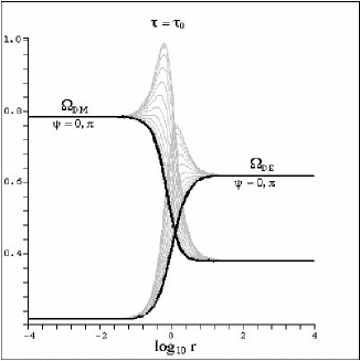
Figure 5: The figure illustrates the effects of anisotropy through the dependence of the profiles of $\Omega_{\textrm{\tiny{DE}}}$ and $\Omega_{\textrm{\tiny{DM}}}$, along $\tau=\tau_{0}$, on the off–center “observation” angle $\psi$. Free parameters are given by (64). The thick black curves correspond to $\psi=0,\pi$, while the gray curves provide the profiles of $\Omega_{\textrm{\tiny{DE}}}$ and $\Omega_{\textrm{\tiny{DM}}}$ for various other values of $\psi$. In particular, the larger “peaks” of these parameters occur for $\psi=\pi/2,3\pi/2$ and around $r\sim 1$. Notice how these effects of anisotropy are negligible in the overdensity region around $r=0$ and in the cosmic background for large $r$. For the deceleration parameter $q$ these effects are negligible for all $r$.

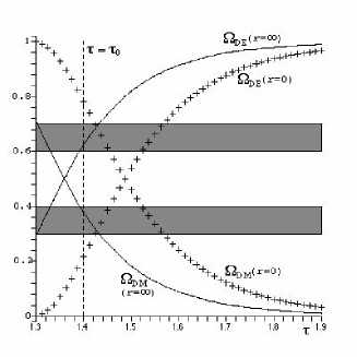
Figure 6: The figure illustrates the effects of inhomogeneity by showing how the time evolution of $\Omega_{\textrm{\tiny{DE}}}$ and $\Omega_{\textrm{\tiny{DM}}}$ (for $\psi=0$) is very different along the center of the overdensity at $r=0$ (crosses) and in the cosmic background ($r\to\infty$, solid curves). The free parameters are given by (64). Notice how in the present cosmic era ($\tau=\tau_{0}$) DE dominates over DM in the cosmic background, but DM dominates over DE in the center.

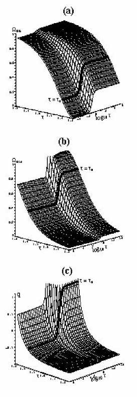
Figure 7: The figures illustrate the full dependence of $\Omega_{\textrm{\tiny{DE}}},\,\Omega_{\textrm{\tiny{DM}}}$ and $q$ on $\tau$ and $r$ (panels (a), (b) and (c)) for $\psi=0$ and with free parameters given by (64). The thick black curves denote the hypersurface of present cosmic time $\tau=\tau_{0}$. The figures clearly show the differences among the overdense region around $r=0$, the cosmic background for large $r$ and the transition zone between them around $r\sim 1$. As in the previous figure, it is evident that DE dominates over DM in the cosmic background, but DM dominates over DE in the center, with both converging as $\tau\to\infty$ to asymptotically homogeneous states with values $\Omega_{\textrm{\tiny{DE}}}\to 1,\,\Omega_{\textrm{\tiny{DM}}}\to 0$. Notice in (c) how the deceleration parameter, $q$, is negative in the cosmic background (accelerating universe), but is positive in the overdense region where the dynamics of local gravity should not be repulsive.

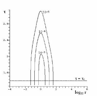
Figure 8: Level curves of the ratio $\sqrt{6}\Sigma/\Theta$. Free parameters are those given by (64). Notice that condition (52) is satisfied for most of the range of $r$ at $\tau=\tau_{0}$, failing to hold only in the transition ($r\sim 1)$ between the overdensity and the cosmic background.

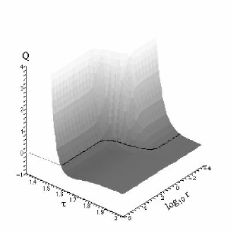
Figure 9: The interaction function $Q(\tau,r)$ given by (66). Free parameters are given by (64) and the level curve $Q=0$ is the thick black curve. Notice how $Q>0$ in the present cosmic era (DE transfers energy to DM), then changes sign (DM transfers energy to DE), with $Q\to 0$ for large $\tau$, thus indicating an asymptotic state in which DE and DM only interact gravitationally.

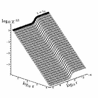
Figure 10: Qualitative logarithmic plot of the coupling function $\chi^{-1/2}$ defined by (71), with $\xi\propto 1/r^{2}$ and free parameters given by (64). The hypersurface $\tau=\tau_{0}$ is displayed as a thick black curve. Notice the clear power law time dependence of $\chi^{-1/2}$, just slightly modulated by the spacial dependence. This indicates that $\chi=\chi(\phi)$ holds approximately for a scalar field associated with (54) and (67).

The efects of anisotropy emerge in the dependence of ${\cal{H}}$, as given by (57), on the off–center “observation angle” $\psi$. This implies dependence on $\psi$ for $\Omega_{\textrm{\tiny{DE}}},\,\Omega_{\textrm{\tiny{DM}}},\,q$. Considering the free parameter values

$$T^{*}=0,\quad f^{*}=100,\quad\delta=200,\quad\gamma=0.15,$$ (64)

complying with the cosmic background ranges (63), figure 5 displays $\Omega_{\textrm{\tiny{DE}}}$ and $\Omega_{\textrm{\tiny{DM}}}$, evaluated at $\tau=\tau_{0}$, as a function of $\log_{10}r$ for assorted fixed values of $\psi$. The same profiles of $\Omega_{\textrm{\tiny{DE}}}$ and $\Omega_{\textrm{\tiny{DM}}}$ occur for $\psi=0$ and $\psi=\pi$ (thick black lines) and, in general for any two values of $\psi$ that differ by a phase of $\pi$, with the highest “peaks” corresponding to gray curves with $\psi=\pi/2$ and $\psi=(3/2)\pi$. This singles out two “preferential” distinctive directions: one along the axis $\psi=0,\,\pi$ and the other along $\psi=\pi/2,\,(3/2)\pi$. This is a clear representation of a quadrupole pattern, as expected for a geodesic but shearing 4-velocity ellis ; HMM . Also, as revealed by figure 5, the curves for the various $\psi$ differ from each other only in the transition region near $r\sim 1$, thus the effects of this quadrupole anisotropy are negligible near the center of the local overdensity and in the cosmic background asymptotic region.

The effects of inhomogeneity are illustrated by figure 6, for the same parameters (64) but keeeping $\psi=0$ fixed, by plotting $\Omega_{\textrm{\tiny{DE}}}$ and $\Omega_{\textrm{\tiny{DM}}}$ as a function of $\tau$ for $r=0$ (crosses) and $r=\infty$ (solid lines). Notice how for the present cosmic era, $\tau=\tau_{0}$, we have $\Omega_{\textrm{\tiny{DE}}}$ dominating at the cosmic background region ($r\to\infty$), but $\Omega_{\textrm{\tiny{DM}}}$ dominates in the overdensity region ($r=0$). This effect of inhomogeneity can be further appretiated in figures 7a, 7b and 7c, displaying $\Omega_{\textrm{\tiny{DE}}}$,  $\Omega_{\textrm{\tiny{DM}}}$ and $q$ as functions of $\tau$ and $\log_{10}r$ for $\psi=0,\,\pi$ and using the free parameters (64). It is particularly interesting to remark how as $\tau$ grows we have:   $\Omega_{\textrm{\tiny{DE}}}\to 1$, $\Omega_{\textrm{\tiny{DM}}}\to 0$ and $q\to-1/2$ for all $r$, as expected for a DE dominated asymptotically future scenario and associated with an ever accelerating universe that follows a “repulsive” dynamics. However, in the present cosmic era (thick black curve) this repulsive accelerated dynamics on which $\Omega_{\textrm{\tiny{DE}}}$ dominates and $q<0$ only happens in the cosmic background region, with $\Omega_{\textrm{\tiny{DM}}}>\Omega_{\textrm{\tiny{DE}}}$ and $q>0$ (i.e. “attractive” dynamics) in the local overdensity region with a relatively large DM density contrast $\delta=200$.

Conditions (52) and (53) place stringent limits on large scale deviations from homogeneity and anisotropy, but these bounds do not apply to local values of these quantities. It is interesting to plot these quantities for the cases depicted in the previous figures, all characterized by (54), (55), (60) and (64). Figure 8 depicts level curves of the logarithm of the shear to expansion ratio of (52), with $\Theta$ and $\Sigma$ given by (21)–(24). Even considering the relatively large value $\delta=200$, condition (52) holds througout most of the coordinate range $(\tau,r)$ including the far range “cosmological background” region of large $r$ and the local overdensity region near the symmetry center $r=0$, so that for the present cosmic time $\tau=\tau_{0}$ it only excludes the relatively small scale local region around $r\sim 1$ that marks the “transition” from the local overdensity to the cosmic background. However, a choice like $\delta=0.01$ would yield similar level curves, but with values three orders of magnitude smaller, thus denoting a state of almost global homogeneity, since (52) would hold in almost all local scales in $\tau=\tau_{0}$. A graph that is qualitatively very similar to that of figure 8 emerges for condition (53).

This difference between the dynamics of local inhomogeneities and that of the cosmic background cannot be appretiated in such a striking and spectacular way if one examines DE and DM sources by means of the usual FLRW models and their linear perturbations.

X Interaction between the mixture components

As we mentioned before, the two mixture components: DM (inhomogeneous dust) plus DE (homogeneous fluid) are not separately conserved. Considering (21) and (23), the energy balance for the total energy–momentum tensor,  $\dot{e}+(e+p)\,\Theta=0$,   can be written in terms of the DM and DE components as

$$\left[\dot{\rho}+\rho\left(\,3\,H+{\cal{Z}}\,\dot{T}\right)\right]+\left[\dot{\mu}+(\mu+p)\left(\,3\,H+{\cal{Z}}\,\dot{T}\right)\right]=0,$$ (65)

Since each term in square brackets in the left hand side of (65) corresponds to the energy balance of each mixture component alone, a self–consistent form for describing the interaction between the latter is given by

$$\dot{\mu}+(\mu+p)\left[\,3\,H+{\cal{Z}}\,\dot{T}\right] = -Q,$$ (66a)

$$\dot{\rho}+\rho\left[\,3\,H+{\cal{Z}}\,\dot{T}\right]\ = Q,$$ (66b)

where $Q=Q(t,r)$ is the interaction term. Since the physics behind DM and DE remains so far unknown, we cannot rule out the existence of such interaction. Notice that once a given model has been determined by specifying an “equation of state” $p=p(\mu)$ and a form for $f=f(r)$, as we have done in the previous sections, this interaction term would also be fully determined. In general, if the interaction term in (66) is a negative valued function, then DM transfers energy into the DE and viceverza. Considering the free parameters given by (54), (60) and (64), we plot in figure 9 the interaction term $Q$ in (66), as a function of $\tau$ and $\log_{10}r$. Notice that $Q$ is initially positive and remains so today (DE trasfers energy to DM at $\tau=\tau_{0}$) but will change sign in a future time (DM trasfers energy to DE), tending to zero asymptotically as $\tau\to\infty$. Thus, the time–asymptotic state is that of only gravitational interaction between DE and DM (i.e. separate conservation of each component).

However, the relevant question is not so much the explicit functional form of $Q$, but its interpretation in terms of a self–consistent physical theory that would be regulating the interaction between DM and DE. In fact, one of the challenges of modern cosmology is to propose such a self–consistent theoretical model of this interaction, while agreeing at the same time with the experimental and observational data. In this context, the interaction between DM and DE has been considered, using homogeneous FLRW cosmologies, in trying to understand the so–called “coincidence problem”, that is, the suspiciously coincidental fact the DE and DM energy densities are of the same order of magnitude in our present cosmic era amendola ; coinc1 ; Q-int1 ; Q-int2 ; Q-int3 ; Q-int4 ; Q-int5 .

If the homogeneous DE fluid corresponds to a quintessense scalar field, $\phi=\phi(t)$, with self-interaction potential $V(\phi)$, we have instead of (54):

$$\mu\ =\ \frac{\dot{\phi}^{2}}{2}+V(\phi),\qquad p\ =\ \frac{\dot{\phi}^{2}}{2}-V(\phi).$$ (67)

In this case, the interaction term in (66) can be associated with a well motivated non–minimal coupling to the DM component. Consider a scalar-tensor theory of gravity, where the matter degrees of freedom and the scalar field are coupled in the action through the scalar-tensor metric $\chi(\phi)^{-1}g_{ab}$kaloper :

$$S_{\textrm{ST}}\ =\ \int d^{4}x\sqrt{|g|}\{\frac{R}{2}-\frac{1}{2}(\nabla\phi)^{2}$$

$$+\ \chi(\phi)^{-2}{\cal L}_{m}(\nu,\nabla\nu,\chi^{-1}g_{ab})\},$$ (68)

where $\chi(\phi)^{-2}$ is the coupling function, ${\cal L}_{m}$ is the matter Lagrangian and $\nu$ is the collective name for the matter degrees of freedom. Equations (66) become

$$\ddot{\phi}+\dot{\phi}\,\left[\,3\,H+{\cal{Z}}\,\dot{T}\right]\ = -\frac{\hbox{d}V}{\hbox{d}\phi}\ +\frac{\rho}{2\dot{\phi}}\frac{\dot{\chi}}{\chi},$$ (69a)

$$\dot{\rho}+\rho\left[\,3\,H+{\cal{Z}}\,\dot{T}\right]\ = \ -\frac{\rho}{2}\;\frac{\dot{\chi}}{\chi}.$$ (69b)

so that, the coupling function $\chi(\phi)$ and the interaction term $Q$ are related by

$$Q=-\frac{\rho}{2}\;\frac{\dot{\chi}}{\chi}.$$ (70)

Therefore, once we determine a given model, so that $Q$ can be explicitly computed, we can use (70) to find the the coupling function $\chi$ that allows us to relate the underlying interaction with the theoretical framework associated with the action (68).

For the models under consideration, we can integrate (in general) the constraint (70) with the help of (15), (18), (19), (21), (69) and using $\Theta=(d/dt)\,[\ln(Y^{2}\,Y^{\prime})]$. This yields

$$\chi^{-1/2} = \ \xi(r)\,\rho\,Y^{2}\,Y^{\prime}$$

$$= \frac{2c_{0}\,H_{0}\,r^{2}\,\xi(r)}{3\,a^{3}}\,\frac{d}{dt}\,\left[(2\,f\,F\,T+f+F)\,R^{3}\right],$$

where $\xi(r)$ is an arbitrary function that emerges as a constant of integration. Notice that the models require $\phi=\phi(t)$, so that the assumption $\chi=\chi(\phi)$ implies $\chi=\chi(t)$. However, from (LABEL:chi), we have (in general) $\chi=\chi(t,r)$, with the case $\chi=\chi(t)$ occurring for the following particular cases, associated with very special forms of $f$ and $\xi$

$$F = 0,\qquad f\propto r^{-3/2},\quad\xi\propto r^{-1/2},$$ (72a)

$$\Rightarrow \chi^{-1/2}\propto\ H,$$

$$f+F = 0,\qquad f\propto r^{-3},\quad\xi\propto r^{4},$$ (72b)

$$\Rightarrow \chi^{-1/2}\propto\ \dot{T}+3\,TH$$

or, if $F\neq 0$ and $f+F\neq 0$, then $f$ and $\xi$ must be obtained from the constraints:

$$\frac{3}{2}\frac{f^{\prime\prime}}{f}+r\frac{f^{\prime}{}^{2}}{f^{2}}+\frac{3f^{\prime}}{f}+\frac{6}{r}=0,$$

$$\frac{\xi\,^{\prime}}{\xi}=-\frac{6f+6\,rf^{\prime}+r^{2}\,f^{\prime\prime}}{r(r\,f^{\prime}+3f)}.$$ (73)

However, since (72) and (73) yield very special forms of $f,\,\xi$ and of $\chi$, we prefer to apply (68) under the most general assumption that the coupling function $\chi$ should be a function of $\phi$ and of position, i.e. $\chi=\chi(\phi(t),r)$, as given by (LABEL:chi) for suitable forms of the free functions $f$, $H$ and $T$ (thus, $\phi$ and $V(\phi)$), hence $\xi$ can be considered a wholly arbitrary function. Considering the free parameters given by (54), (55), (60) and (64), and taking $\xi\propto 1/r^{2}$, figure 10 illustrates qualitatively how the coupling function $\chi^{-1/2}$ given by (LABEL:chi) follows a power law time dependence, slightly modulated by the change of local DM densities from the local overdensity region to the low density cosmic background. Since the scalar field (67) that corresponds to the equation of state (54) and the parameters (55) also exhibits a power law time dependence CJSF , we do have approximately $\chi=\chi(\phi)$, as required by (68).

However, figure 10 is just a qualitative plot. We should point out that relating the interaction term, $Q$, to the formalism represented by (68) is strictly based on the formal similitude between the field equations derived from the action (68), on the one hand, and equations (66) and (67), on the other. Also, the interaction between DM and DE in the context of (68) is severely constrained by experimental tests in the solar system will . A more detailed and carefull examination of the relation between $\chi$ and $\phi$ that incorporates properly these points, as well as the application of (68) to the models presented here, will be undertaken in future papers.

XI Conclusion.

We have presented a class of inhomogeneous cosmological models whose source is an interacting mixture of DM (dust) and a generic DE fluid. The relevance of the present paper emerges when we realize that there are surprisingly few studies in which DE and DM are the sources of inhomogeneous and anisotropic spacetimes (see Qinhom ), as practically all study of the dynamical evolution of these components is carried on in the context of homogeneous and isotropic FLRW cosmologies or linear perturbations on a FLRW background. There are also very few papers that examine the possibility of non–gravitational interaction between DE and DM.

Once we assume or prescribe an “equation of state” (i.e. a relation between pressure, $p$, and matter–energy density, $\mu$, of the DE fluid), we have a specific DE model (quintessense scalar fields, tachyonic fluid, etc) and all the time–dependent parameters can be determined by solving two coupled differential equations reminissent of FLRW fluids. Since the spacial dependence of all quantities is governed by the function $f=f(r)$, once the latter is selected the models become fully determined (though, various important regularity conditions must be also satisfied: see section VI). In order to work out this process we chose the simple “gamma law” equation of state: $p=(\gamma-1)\mu$ (equation (54)), leading to analytic forms for all relevant quantities, including the main observational parameters, $\Omega_{\textrm{\tiny{DE}}},\,\Omega_{\textrm{\tiny{DM}}}$ and $q$. Our choice for a DE fluid complying with (54) is equivalent to a scalar field with exponential potential, satisfying a scaling power law dependence on $t$ CJSF . Although this is a very idealized quintessense model, our aim has been to use it as a guideline that illustrates how more sophisticated DE scenarios can be incorporated in future work involving the models.

As we have mentioned in section VI, the models homogeneize and isotropize asymptotically in cosmic time for all fundamental observers and/or assumptions on the DE fluid, thus they are well suited for studying the interaction between DE and DM in the context of the evolution of large scale inhomogeneities (of the order of the scale of homogeneity $\sim 100-300$ Mpc). By selecting appropriate boundary conditions, we can examine inhomogeneities at various scales and/or asymptotic conditions (see figures 2 and 3). In particular, we have explored the case of a local DM overdense region, whose scale can be arbitrarily fixed and with an asymptotic behavior that accurately converges to a cosmic background characterized by observational parameters that fit currently accepted observational constraints: $0.6<\Omega_{\textrm{\tiny{DE}}}<0.8,\,\,0.2<\Omega_{\textrm{\tiny{DM}}}<0.4$ and $q\approx-0.5$ (see figure 4). As illustrated by the various graphical examples that we have presented, this interplay between a local overdensity, a cosmic background and a transition region between them, shows in a spectacular manner how inhomogeneity and anisotropy lead to interesting and important information that cannot be appretiated in models based on FLRW metrics and/or linear perturbations. For example, as revealed by figure 5, the effect of anisotropy emerges as a dependence of observational parameters on local observation angles in “off center postions”, an effect which is only significant in the transition between the overdensity and the cosmic background. On the other hand, as shown by figures 6-8, inhomogeneity allows for radically different ratios between DM and DE in the overdensity and the cosmic background, so that DM dominates over DE, locally, in the overdense region, as a contrast with DE dominating DM, asymptotically, in the cosmic background (as expected). Also, while $q$ is negative in the cosmic (DE dominated) background, thus denoting the expected “repulsive” accelerated expansion at large scales, we have $q>0$ along smaller scales in the local overdensity. For all parameters there is a smooth convergence between local and asymptotic values in the transition region.

We have also examined the non–gravitational interaction between DE and DM. Ploting the interaction term, $Q$, (figures 9) shows that energy flows from DE to DM at the present cosmic era, with the flow reversing direction in the future and evolving towards an asymptotic future state characterized by pure gravitational interaction: $Q\to 0$. If we take the DE fluid to be a quintessense scalar field, the DE vs DM interaction can be incorporated to the theoretical framework of an action like (68), associated with a non–minimal coupling of scalar fields and DM. Since DM is inhomogeneous while the scalar field is homogeneous, only for some particular forms of spacial dependence (i.e. the function $f$) we obtain a coupling function expressible as $\chi=\chi(\phi)$. In general, we have to allow for the possibility that $\chi=\chi(\phi(t),r)$, but as shown by figure 10, the spacial dependence of $\chi$ under the assumption (54) (scalar field with exponential potential) mantains a power law dependence that is qualitatively very similar to that shown in the homogeneous case. However, we have examined this interaction just in qualitative terms, with the purpose of illustrating the methodology to follow in future applications.

As guidelines for future work, we have the application of the models to more sophisticated and better motivated DE formalisms, perhaps in the context of the “coincidence” problem amendola ; coinc1 ; Q-int1 ; Q-int2 ; Q-int3 ; Q-int4 ; Q-int5 . An interesting development would be the study of the case $K\neq 0$, in which hypersurfaces of constant $t$ (rest frames) have nonzero curvature (see section II). This requires solving the non–linear equation (5), which would certainly need numerical techniques and perhaps assuming an homothetic symmetry that could reduce it to an ordinary differential equation. The advantage would be the possibility of describing the effects of DE on structure formation, since a DM overdense region with $K>0$ could collapse, locally, as a DE dominated cosmic background with $K\leq 0$ expands. Finally, we have examined the DE/DM mixtures that can be constructed with the Szekeres–Szafron models of “class 1”, as those of old2F2 , thus it still remains pending the study of “class 2” models like those of old2F1 .

- (1) R.R. Caldwell, R. Dave and P.J. Steinhard, Phys. Rev. Lett., 80, 1582, (1995); M.S. Turner and M. White, Phys. Rev. D 56, R4439, (1997); Bahcall et al, Science, 284, 1481, (1999); A. G. Riess, et al., Astron. J. 116, 1009-1038 (1998); S. Perlmutter, et al., Astrophys. J. 517, 565-586 (1999).
- (2) A. G. Riess, et al., Astrophys. J., 536, 62 (2000); A. G. Riess, et al., Astrophys. J., 560, 49-71 (2001); J. L. Tonry, et al., Astrophys. J., 594, 1-24 (2003); A. G. Riess, et al., Astrophys. J., 607, 665-687 (2004); M. Tegmark et. al. asto-ph/0310723; A. Upadhye, M. Ishak and P.J. Steinhardt, asto-ph/0411803.
- (3) T. Padmanabhan, Phys Rept, 380, 235–320, (2003).
- (4) J.A.S. Lima, Braz.J.Phys., 34, 194–200, (2004).
- (5) L. Amendola, Phys. Rev. D62 (2000) 043511; 063508 (astro-ph/0005070).
- (6) L. P. Chimento, A. S. Jakubi and D. Pavón, Phys. Rev. D, 62, 063508, (2000).
- (7) W. Zimdahl, D. Pavón and L.P. Chimento, Phys Lett B, 521, 133, (2001).
- (8) L.P. Chimento et. al., Phys Rev D, 67, 083513, (2003).
- (9) L.P. Chimento and A.S. Jakubi, Phys Rev D, 67, 087302, (2003); L. P. Chimento, A. S. Jakubi and D. Pavon, Phys. Rev. D, 67 (2003) 087302.
- (10) W. Zimdahl and D. Pavón, Gen Rel Gravit, 35, 413, (2003).
- (11) L.P. Chimento and A.S. Jakubi, Phys Rev D, 69, 083511, (2004).
- (12) A. Krasinski, Inhomogeneous Cosmological Models, Cambridge University Press, 1997.
- (13) J.A.S. Lima and J. Tiomno, Gen Rel Gravit, 20, 1019, (1988)
- (14) R.A. Sussman, Classical and Quantum Gravity, 9, 1881-1915, (1992).
- (15) J. J. Halliwell, Phys. Lett. B, 185, 341 (1987); C. Wetterich, Nucl. Phys. B, 302, 668 (1988); D. Wands, E. J. Copeland, and A. R. Liddle, Ann. N.Y. Acad. Sci., 688, 647 (1993). P. G. Ferreira and M. Joyce, Phys. Rev. D, 58, 023503 (1998); L.P. Chimento and A.S. Jakubi, Int J Mod Phys D, 5, 313, (1996).
- (16) S.W. Goode and J. Wainwright, Phys Rev D, 26, 3315, (1982).
- (17) G.F.R Ellis and H. van Elst, Cosmological Models, Cargèse Lectures 1998, gr-qc/9812046.
- (18) N. Humphreys, R. Maartens and D. Matravers, Ap J, 477, 47, (1997).
- (19) R. Maartens, G.F.R. Ellis and W.R. Stoeger, Phys Rev D, 51, 1525-1535, (1995); J. Barrow and R. Maartens, Phys Rev D, 59, 043502, (1999).
- (20) C. M. Will, Theory and Experiment in Gravitational Physics (Cambridge University Press, 1993); gr-qc/0103036.
- (21) N. Kaloper and K. A. Olive, Phys. Rev. D57 (1998) 811-822 (hep-th/9708008); L. Amendola, Phys. Rev. Lett. 93 (2004) 181102 (hep-th/0409224).
- (22) L. P. Chimento, A. S. Jakubi and D. Pavón, Phys Rev D, 60, 103501, (1999).