Star formation rates and mass distributions in interacting galaxies

We present a systematic investigation of the star formation rate (hereafter SFR) in interacting disk galaxies. We determine the dependence of the overall SFR on different spatial alignments and impact parameters of more than 50 different configurations in combined N-body/hydrodynamic simulations. We also show mass profiles of the baryonic components. We find that galaxy-galaxy interactions can enrich the surrounding intergalatic medium with metals very efficiently up to distances of several 100 kpc. This enrichment can be explained in terms of indirect processes like thermal driven galactic winds or direct processes like ’kinetic’ spreading of baryonic matter. In the case of equal mass mergers the direct -kinetic- redistribution of gaseous matter (after 5 Gyr) is less efficient than the environmental enrichment of the same isolated galaxies by a galactic wind. In the case of non-equal mass mergers however, the direct -kinetic- process dominates the redistribution of gaseous matter. Compared to the isolated systems, the integrated star formation rates (ISFRs) ($\int_{t\,=\,0\,Gyr}^{t\,=\,5\,Gyr}\textnormal{SFR(t)}dt$) in the modelled interacting galaxies are in extreme cases a factor of 5 higher and on average a factor of 2 higher in interacting galaxies. Co-rotating and counter-rotating interactions do not show a common trend for the enhancement of the ISFRs depending on the interaction being edge-on or face-on. The latter case shows an increase of the ISFRs for the counter-rotating system of about 100%, whereas the edge-on counter-rotating case results in a lower increase ($\sim$ 10%). An increase in the minimum separation yields only a very small decrease in the ISFR after the first encounter. If the minimum separation is larger than $\sim 5\times$ the disk scale length R_d the second encounter does not provide an enhancement for the ISFR.

1 Introduction

Optical, far-infrared and radio observations in the last decades have shown that the global star formation rate (SFR) [$M_{\sun}$/yr] in interacting disk galaxies is enhanced in comparison to isolated galaxies (Bushouse H. A. 1987; Sulentic 1976; Stocke 1978). Modern imaging surveys like GEMS (Rix et al. 2004) or COMBO17 (Bell et al. 2004) reveal the importance of mergers on the evolution of red-sequence/early-type galaxies and constrain therefore hierarchical models of galaxy formation and evolution. Studying single objects like elliptical galaxies with dust and gas layers like NGC6255 (Morganti et al. 2000) shows us the complexity of merged systems very impressively. Kauffmann et al. 2004 concluded that the majority of massive red galaxies are the result of mergers, in which rapidly stars are formed and gas is depleted. To study the dynamics and evolution of stellar populations of merging systems observations as well as simulations are necessary.
Whereas former numerical investigations had a special emphasis on modelling observed interacting systems, like NGC7252 (Mihos et al. 1998), we are interested in the dependence of the star formation rates on interaction parameters like spatial alignment and minimum separation. Cox et al. (2004) investigated galaxy mergers with a special emphasis on the heating process of gas due to shocks. Simulations including accretion onto supermassive black holes in merging galaxies (Springel et al. 2005) and the resulting suppression of star formation and the morphology of the elliptical remnant are the newest improvements on this topic. It was recently investigated by Springel & Hernquist (2005) wether galaxy mergers always end up in an elliptical galaxy or not. They have shown that under certain circumstances (e.g. gas rich disk) the merger remnant can be a star forming disk galaxy. As the global star formation rate will increase the overall supernova rate (SNR) [SN/yr] in close pairs of galaxies this increases the mass loss rates (MLR) [$M_{\sun}$/yr] of such systems due to supernova driven mass loaded galactic winds (Colina, Lipari & Macchetto 1991). Modern X-ray astronomy has revealed the non-primordial metallicity of the intra-cluster medium (ICM) (Tamura et al. 2004). In addition metal maps of galaxy clusters show that the metals are not uniformly distributed over the ICM (Schmidt et al. 2002; Furusho et al. 2003; Sanders et al. 2004; Fukazawa et al. 2004). As heavy elements are produced in stars the processed material must have been ejected by cluster galaxies into the ICM. Ram-pressure stripping (Gunn & Gott 1972), galactic winds (De Young 1978) and direct enrichment by galaxy-galaxy interactions (Gnedin 1998) present possible transport mechanisms. De Lucia et al. (2004) used combined N-body and semi-analytical techniques to model the intergalactic and intra-cluster chemical enrichment due to galactic winds. As mergers can cause superwinds due to enhanced star formation they play an important role for enrichment processes. Tornatore et al. (2004) did Tree+SPH simulations of galaxy clusters to study the metal enrichment of the intra-cluster medium. All these different approaches need a proper treatment of galaxy mergers. In this paper we present a detailed study on the dependence of the SFRs of interacting galaxies on the spatial orientation and the impact parameter. We show that not only galactic winds, due to an enhanced star formation, can enrich the intergalactic or intracluster medium, but direct redistribution due to the interaction process has to be taken into account as well. In order to investigate the duration and strength of the SFRs in interacting galaxies we did SPH simulations with an updated version of GADGET (Springel et al. 2001), which employs the entropy conservative formulation (Springel & Hernquist 2002). Spiral galaxies with different spatial alignments were thereby put on different collision trajectories.

2 The galaxy model

The simulated galaxies were modelled with an initial condition generator for disk galaxies developed by Volker Springel. A detailed description and analysis of the method and the influence of the initial conditions on the evolution of the model galaxies can be found in Springel et al. (2004). The mass and the virial radius of the halo are given by

$$M_{200}=\frac{v^{3}_{200}}{10\,G\,H(z)}\qquad\mbox{and}\qquad r_{200}=\frac{v_{200}}{10\,H(z)}$$ (1)

with $H(z)$ being the Hubble constant at redshift z and $G$ the gravitational constant. We built three different spiral galaxies, two of them with a bulge and one without a bulge. See Table 1 for the properties of the model galaxies. To allow for resolution studies each model galaxy was investigated with different particle numbers, see Table 2. Figure 1 shows images of the model galaxies at 0.5 Gyr after the start of the simulation. The distribution of both the gas and the collisionless particles in the disk are shown edge on as well as face on. The star forming knots in the disk are visible.

Table 1: Properties of the model galaxies

Properties	Galaxy A	Galaxy B	Galaxy C
halo concentration1	5	5	5
circular velocity $v_{200}$ [km/s] 2	160	80	160
spin parameter $\lambda$ 3	0.05	0.05	0.05
disk mass fraction4	0.05	0.05	0.05
bulge mass fraction4	0	0	0.025
bulge size5	0	0	0.5
gas content in the disk6	0.25	0.25	0.25
disk thickness7	0.02	0.02	0.02
HI gas mass fraction8	0.5	0.5	0.5
total mass [$M_{\sun}$]	1.3375x1011 $h^{-1}$	1.67188x1010 $h^{-1}$	1.3375x1011 $h^{-1}$
disk scale length [kpc]	4.50622$h^{-1}$	2.25311$h^{-1}$	3.91342$h^{-1}$

¹…$c\equiv\frac{r_{200}}{r_{s}}$ ($r_{s}$..scale radius for dark matter halo density profile $\rho(r)=\rho_{crit}\frac{\delta_{0}}{(r/r_{s})(1+r/r_{s})^{2}}$)
²…circular velocity at $r_{200}$
³…$\lambda=J|E|^{1/2}G^{-1}M^{-5/2}$
⁴…of the total mass (baryonic and non baryonic matter)
⁵…bulge scale length in units of disk scale length
⁶…relative content of gas in the disk
⁷…thickness of the disk in units of radial scale length
⁸…in comparison to the total gas mass

Table 2: Particle numbers and mass resolution

	Resolution H	Resolution M	Resolution L
Halo	50000	30000	10000
Disk collisionless	35000	20000	7000
Gas in disk	35000	20000	7000
Total number	120000	70000	24000
Mass resolutions - softening length
[$h^{-1}$ $M_{\sun}$/particle] / [$h^{-1}$ kpc]
Galaxy A Halo	$2.5\times 10^{6}$ - 0.2	$4.2\times 10^{6}$ - 0.4	$1.3\times 10^{7}$ - 0.6
Galaxy A Disk	$1.9\times 10^{5}$ - 0.05	$3.3\times 10^{5}$ - 0.1	$9.5\times 10^{5}$ - 0.2
Galaxy A Gas	$4.7\times 10^{4}$ - 0.05	$8.4\times 10^{4}$ - 0.1	$2.4\times 10^{5}$ - 0.2
Galaxy B Halo	$3.2\times 10^{5}$ - 0.2	$5.3\times 10^{5}$ - 0.4	$1.6\times 10^{6}$ - 0.6
Galaxy B Disk	$2.4\times 10^{4}$ - 0.05	$4.2\times 10^{4}$ - 0.1	$1.2\times 10^{5}$ - 0.2
Galaxy B Gas	$6.0\times 10^{3}$ - 0.05	$1.1\times 10^{4}$ - 0.1	$3.0\times 10^{4}$ 0.2
Halo	50000	30000	10000
Disk collisionless	35000	20000	7000
Gas in disk	35000	20000	7000
Bulge particles	20000	10000	3500
Total number	140000	80000	27500
Mass resolutions / softening length
[$M_{\sun}$/particle] / [$h^{-1}$ kpc]
Galaxy C Halo	$3.5\times 10^{6}$ - 0.2	$6.2\times 10^{6}$ - 0.4	$1.8\times 10^{7}$ - 0.6
Galaxy C Disk	$1.9\times 10^{5}$ - 0.05	$3.3\times 10^{5}$ - 0.1	$9.5\times 10^{5}$ - 0.2
Galaxy C Bulge	$1.7\times 10^{5}$ - 0.05	$3.3\times 10^{5}$ - 0.1	$9.5\times 10^{5}$ - 0.2
Galaxy C Gas	$4.7\times 10^{4}$ - 0.05	$8.4\times 10^{4}$ - 0.1	$2.4\times 10^{5}$ - 0.2

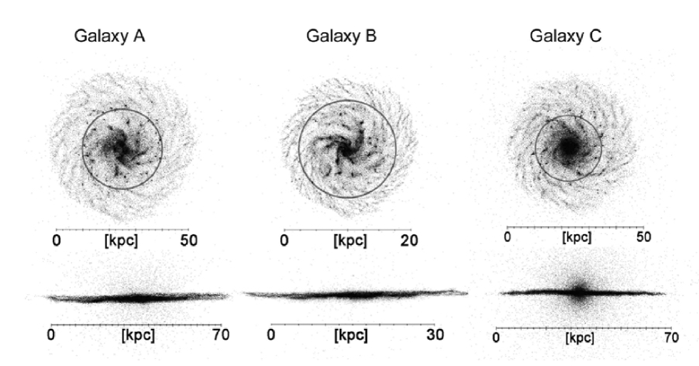
Figure 1: Model galaxies A, B and C. The properties of the galaxies are listed in Table 1. The upper panels show gas and collisionless particles in the disk seen face on and the lower panel shows the galaxies edge on. The ring in the upper panel marks the optical radius $R_{opt}=3.2R_{d}$ ($R_{d}$…disk scale length). The knots in the disk represent star forming regions resulting from gas overdensities. All galaxies are shown at the same time ( 0.5 Gyr after simulation start). The images correspond to the model galaxies with the highest resolution as given in Table 22.

3 The star formation and feedback model

To simulate the feedback of supernovae (SNe) on the interstellar medium (ISM) we applied the so called ”hybrid” method for star formation and feedback which was introduced by Springel & Hernquist (2003). In this hybrid approach condensed cold gas clouds coexist in pressure equilibrium with a hot ambient gas. Labelling the average density of the stars as $\rho_{*}$, the density of the cold gas $\rho_{c}$ and the density of the hot medium $\rho_{h}$, the total gas density in the disk can be written as $\rho=\rho_{h}+\rho_{c}$. Because of the finite number of particles in our simulations $\rho_{*}$ and $\rho$ represent averages over regions of the inter-stellar medium (ISM). The central assumption in this approach is the conversion of cold clouds into stars on a characteristic timescale $t_{*}$ and the release of a certain mass fraction $\beta$ due to supernovae (SNe). This relation can be expressed as

$$\frac{d\rho_{*}}{dt}=\frac{\rho_{c}}{t_{*}}-\beta\frac{\rho_{c}}{t_{*}}=(1-\beta)\frac{\rho_{c}}{t_{*}}.$$ (2)

As a consequence of the fact that released material from SNe is hot gas the cold gas reservoir increases at the rate $\rho_{c}/t_{*}$. In this picture $\beta$ gives the mass fraction of massive stars ($>$ 8 $M_{\sun}$). As in Springel & Hernquist (2003) we adopt a $\beta=0.1$ assuming a Salpeter IMF with a slope of -1.35 in the limits of 0.1 $M_{\sun}$ and 40 $M_{\sun}$. In addition each supernova event releases energy of $1\times 10^{51}$ erg into the ambient medium. This leads to an average return of $\epsilon=4\times 10^{48}$ erg $M_{\sun}^{-1}$. This energy heats the ambient hot medium and evaporates the cold clouds inside the hot bubbles of exploding SNe. The total mass of clouds evaporated can be written as

$$\frac{d\rho_{c}}{dt}|_{EV}=-A\beta\frac{\rho_{c}}{t_{*}}.$$ (3)

The evaporation process is supposed to be a function of the local environment with an efficiency A $\propto\rho^{-4/5}$ (McKee & Ostriker, 1977). The minimum temperature the gas can reach due to radiative cooling is about $10^{4}$ K. The energy balance per unit volume is $\epsilon_{UV}=\rho_{h}*u_{h}+\rho_{c}*u_{c}$ ($u_{h,c}$ energies per unit mass of the cold and hot gas). All this assumptions lead to self regulating star formation due to the conversion of cold gas into stars and the feedback of hot gas into the reservoir of the hot ambient medium, which can cool due to radiative cooling to cold clouds. The rates are finally

$$\frac{d\rho_{c}}{dt}=-\frac{\rho_{c}}{t_{*}}-A\beta\frac{\rho_{c}}{t_{*}}+\frac{1-f}{u_{h}-u_{c}}\Lambda_{net}(\rho_{h},u_{h})\\$$ (4)

$$\frac{d\rho_{h}}{dt}=\beta\frac{\rho_{c}}{t_{*}}+A\beta\frac{\rho_{c}}{t_{*}}-\frac{1-f}{u_{h}-u_{c}}\Lambda_{net}(\rho_{h},u_{h})$$ (5)

where f represents a factor to differentiate between ordinary cooling (f=1) and thermal instability (f=0). $\Lambda_{net}$ is the cooling function (Katz et al., 1996). Equations (4) and (5) give the mass budget for the hot and cold gas due to star formation, mass feedback, cloud evaporation and growth of clouds due to radiative cooling. On the other side the thermal budget can be written as

$$\frac{d}{dt}(\rho_{c}u_{c})=-\frac{\rho_{c}}{t_{*}}u_{c}-A\beta\frac{\rho_{c}}{t_{*}}u_{c}+\frac{(1-f)u_{c}}{u_{h}-u_{c}}\Lambda_{net}$$ (6)

$$\frac{d}{dt}(\rho_{h}u_{h})=\beta\frac{\rho_{c}}{t_{*}}(u_{SN}+u_{c})+A\beta\frac{\rho_{c}}{t_{*}}u_{c}-\frac{u_{h}-fu_{c}}{u_{h}-u_{c}}\Lambda_{net}$$ (7)

with $u_{SN}$ the energy per unit volume from SN explosions. A major assumption is the fixed temperature of cold gas clouds which leads to a constant $u_{c}$. One of the basic equations of the routine is the evolution of the hot phase according to

$$\rho_{h}\frac{du_{h}}{dt}=\beta\frac{\rho_{c}}{t_{*}}(u_{SN}+u_{c}-u_{h})-A\beta\frac{\rho_{c}}{t_{*}}(u_{h}-u_{c})-f\Lambda_{net}.$$ (8)

From observations and other simulations it is evident that a certain fraction of matter can escape the galaxies potential due to thermal and or cosmic ray driven winds due to SNe explosions (Breitschwerdt et al. 1991). This of course leads to a deficit in the mass and energy budget of a galaxy, especially in the case of starbursts. Therefore we applied the same approach as Springel & Hernquist (2003) to model this process. The mass-loss rate of the disk $\dot{M_{w}}$ is proportional to the star formation rate $\dot{M_{*}}$, in particular $\dot{M_{w}}=\eta\dot{M_{*}}$ with $\eta=2$, consistent with the observations of Martin (1999). An additional assumption is that the wind contains a fixed fraction $\chi$ of SN energy. This fixed fraction is assumed to be 0.25. For a more detailed description of the feedback routine see Springel & Hernquist (2003).

4 Resolution study for isolated galaxies

The goal of this work is to investigate the overall SFR evolution of interacting galaxies by varying the spatial alignment and the impact parameter of the interacting galaxies. Therefore firstly the SFR of the isolated galaxies has to be studied, to distinguish which contribution to the global SFR comes from the undisturbed galaxies and which from the interaction. Another major point in numerical simulations is the resolution of the system, ie. the number of particles. Local gas densities define the amount of newly formed stars, therefore resolution and gravitational softening influences the quantitative maximum of the SFR. As we are interested in the relative change of the integrated overall SFR for interacting systems, the absolute value of the maximum of the SFR does not influence the results, as long as the resolution, softenings and feedback parameters are constant for all simulations. Figure 2 gives the evolution of the SFR for the isolated galaxy A with different resolutions (see Table 2). The maximum of the SFR at t $\sim$ 0.3 Gyr is caused to instabilities on the gaseous disk as it begins to rotate and evolves. A detailed stability analysis for disks with different gas masses and equation of state softenings can be found in Springel et al. (2004, section 6). Integrating and normalizing the SFR over a time range of 5 Gyr results for model Galaxy AH 1, for model Galaxy AM 0.7929 and for model Galaxy AL 0.9291. The SFR of a model galaxy with $v_{200}=80$ km/s is two orders of magnitude lower than a model galaxy with $v_{200}=160$. As $v_{200}$ defines the total mass and the size of a system, see equation 1 and 2, the gas content in the disks of model galaxy A and B differ in the order of one magnitude, see Table 1. As a consequence of the lower gas mass and the smaller disk of model galaxy B the induced instabilities result in a smaller overall SFR. Figure 4 shows the gaseous and stellar matter of the isolated model galaxy AM at t=0.5, t=2 and t=4 Gyr.

Figure 2: SFRs for the isolated model galaxies. The labelling Galaxy AM, Galaxy AH and Galaxy AL corresponds to the galaxy properties defined in Tables 1 and 2.

Figure 3: SFRs for all isolated model galaxies given in Table 1 (resolution M, see Table 2).

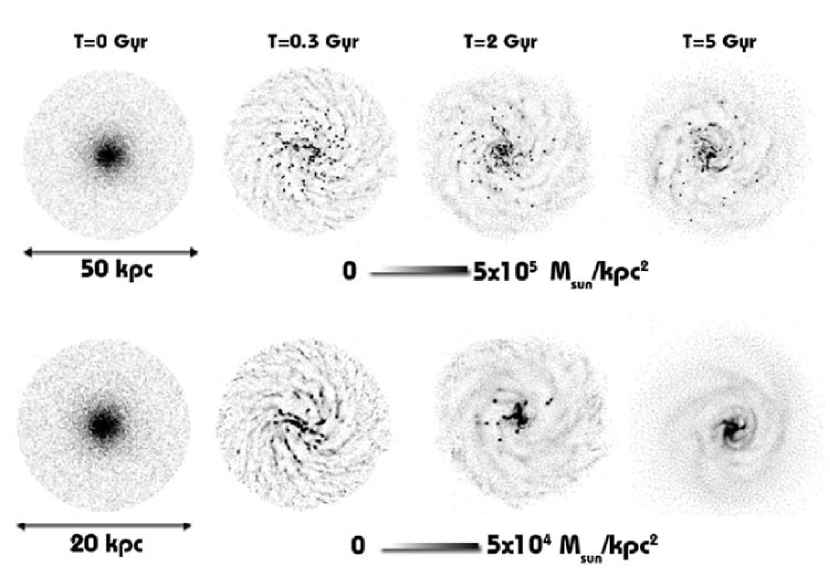
Figure 4: Evolution of the gas particles in the disk for model galaxy AM (upper panel) and BM (lower panel). The star forming overdensities at T=0.3 Gyr and the number decrease of this regions at T=2 (2 Gyr) and T=5 (5 Gyr) can be seen.

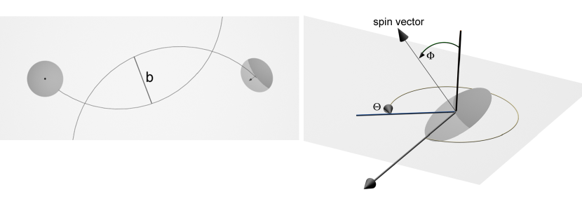
Figure 5: Interaction geometry. The galaxies’ positions and velocities are chosen in such a way that the galaxies are point masses moving on Keplerian orbits. See Duc et al. (2000) for further descriptions.

5 The spatial alignments and impact parameters

The geometry of the interaction was set up in the same coordinate system as in Duc et al. (2000). Figure 5 shows the angles and the trajectories. The galaxies’ positions and velocities were set up as if they were point masses on Keplerian orbits with a minimum separation $\bf{b}$. Tables 3 and 4 list the different angles and impact parameters for our simulations. The alignments were chosen to cover as much interaction geometries as possible. Of course computational time is the limiting factor, therefore the number of different alignments is limited. Special emphasis was put on the investigation of co- and counter-rotating cases and on increasing the minimum separation $\bf{b}$ for simulating fly-bys. All together we did 9 different spatial alignments and 8 different minimum separations for 4 different interacting systems. This leads to an overall of 56 simulations to cover as many interacting scenarios as possible.

Table 3: Interaction parameters for simulations 1-28 and results. Col.2: model galaxy 1; Col. 5: model galaxy 2; Col. 8: maximum separation [kpc]; Col. 9: minimum separation [kpc]; Col. 10: normalized total SF; Col. 11: total SF $<$ 2 Gyr; Col. 12: total SF between 2 Gyr and 3 Gyr; Col. 13: total SF $\geq$ 3 Gyr; Col. 14: gas/stellar mass @ t=0 Gyr; Col. 15: gas/stellar mass @ t=2 Gyr; Col. 16: gas/stellar mass @ t=3 Gyr; Col. 17: gas/stellar mass @ t=5 Gyr; Col. 18: 80% gas mass within radius [kpc]; Col. 19: 80% stellar mass within radius [kpc]; Col. 20: 80% new formed stars within radius [kpc]

Simulation	C 2	$\Phi_{1}$	$\Theta_{1}$	C 5	$\Phi_{2}$	$\Theta_{2}$	C 8	C 9	C 10	C 11	C 12	C 13	C 14	C 15	C 16	C 17	C 18	C 19	C 20
two isolated
galaxies A	A	-	-	A	-	-	-	-	1.001	0.79	0.08	0.13	0.25	0.19	0.19	0.18	-3	-3	-3
Sim 1	A	0	0	A	0	0	200	0	2.79	0.61	0.14	0.25	0.25	0.14	0.12	0.08	5.42	7.23	1.20
Sim 2	A	0	0	A	0	0	200	5	2.75	0.45	0.07	0.48	0.25	0.16	0.15	0.07	1.06	7.45	2.13
Sim 3	A	0	0	A	0	0	200	10	2.60	0.53	0.06	0.41	0.25	0.16	0.15	0.07	2.45	4.23	1.25
Sim 4	A	0	0	A	0	0	200	20	2.75	0.50	0.01	0.49	0.25	0.17	0.16	0.07	1.64	2.82	1.63
Sim 5	A	0	0	A	0	0	200	25	2.65	0.41	0.06	0.53	0.25	0.18	0.17	0.08	0.85	7.97	1.42
Sim 6	A	0	0	A	0	0	200	30	1.85	0.54	0.07	0.39	0.25	0.18	0.17	0.13	0.08	1.23	0.28
Sim 7	A	0	0	A	0	0	200	40	1.24	0.78	0.11	0.11	0.25	0.19	0.18	0.17	-4	-4	-4
Sim 8	A	0	0	A	0	0	200	50	1.09	0.72	0.11	0.16	0.25	0.19	0.18	0.17	-4	-4	-4
Sim 9	A	0	0	A	90	0	200	5	1.77	0.57	0.06	0.35	0.25	0.18	0.17	0.13	4.11	6.17	3.08
Sim 10	A	0	0	A	90	90	200	5	2.45	0.47	0.04	0.49	0.25	0.18	0.17	0.10	1.78	7.12	1.78
Sim 11	A	90	0	A	90	0	200	5	1.13	0.81	0.09	0.10	0.25	0.19	0.18	0.17	2.22	4.44	2.22
Sim 12	A	90	0	A	-90	0	200	5	2.09	0.45	0.07	0.48	0.25	0.19	0.18	0.12	0.10	6.02	0.54
Sim 13	A	0	0	A	45	0	200	5	1.77	0.58	0.07	0.35	0.25	0.18	0.17	0.13	5.03	6.03	3.01
Sim 14	A	45	0	A	45	0	200	5	1.44	0.65	0.07	0.28	0.25	0.18	0.17	0.15	1.69	5.09	0.85
Sim 15	A	-45	0	A	45	0	200	5	2.12	0.45	0.05	0.50	0.25	0.18	0.17	0.11	0.70	6.34	1.17
Sim 16	A	0	0	A	180	0	200	5	2.55	0.55	0.00	0.45	0.25	0.17	0.16	0.09	0.13	8.03	0.76
isolated galaxies
A and B	A	-	-	B	-	-	-	-	1.002	0.79	0.08	0.13	0.25	0.19	0.19	0.18	-3	-3	-3
Sim 17	A	0	0	B	0	0	200	0	1.33	0.77	0.12	0.11	0.25	0.19	0.18	0.17	14.06	8.88	4.07
Sim 18	A	0	0	B	0	0	200	5	1.19	0.78	0.07	0.15	0.25	0.20	0.20	0.19	20.05	11.34	7.91
Sim 19	A	0	0	B	0	0	200	25	1.13	0.73	0.11	0.16	0.25	0.20	0.20	0.19	-4	-4	-4
Sim 20	A	0	0	B	0	0	200	50	1.11	0.74	0.12	0.14	0.25	0.20	0.20	0.19	-4	-4	-4
Sim 21	A	0	0	B	90	0	200	5	1.11	0.72	0.10	0.18	0.25	0.20	0.20	0.19	21.15	12.08	8.63
Sim 22	A	0	0	B	90	90	200	5	1.28	0.68	0.12	0.20	0.25	0.20	0.19	0.18	16.04	10.13	4.60
Sim 23	A	90	0	B	90	0	200	5	1.22	0.73	0.14	0.13	0.25	0.20	0.19	0.18	10.51	8.18	8.18
Sim 24	A	90	0	B	-90	0	200	5	1.18	0.85	0.00	0.15	0.25	0.20	0.19	0.18	12.85	9.64	8.84
Sim 25	A	0	0	B	45	0	200	5	1.13	0.72	0.08	0.20	0.25	0.20	0.20	0.19	20.85	12.75	9.66
Sim 26	A	45	0	B	45	0	200	5	1.23	0.71	0.12	0.17	0.25	0.20	0.19	0.18	15.40	9.86	8.63
Sim 27	A	-45	0	B	45	0	200	5	1.31	0.70	0.11	0.19	0.25	0.20	0.19	0.18	16.00	9.43	6.56
Sim 28	A	0	0	B	180	0	200	5	1.28	0.51	0.10	0.39	0.25	0.20	0.20	0.18	5.39	8.56	2.04

¹….$2\times\int_{t\,=\,0\,Gyr}^{t\,=\,5\,Gyr}SFR_{A}(t)dt=4.4\times 10^{9}$M_☉, this is normalised to 1.
²….$\int_{t\,=\,0\,Gyr}^{t\,=\,5\,Gyr}SFR_{A}(t)dt+\int_{t\,=\,0\,Gyr}^{t\,=\,5\,Gyr}SFR_{B}(t)dt=2.4\times 10^{9}$M_☉, this is normalised to 1.
³….see Table 6 for numbers.
⁴….no merger occurs within simulation time, therefore no cut-off radii are given.

Table 4: Interaction parameters for simulations 29-56 and results. Col.2: model galaxy 1; Col. 5: model galaxy 2; Col. 8: maximum separation [kpc]; Col. 9: minimum separation [kpc]; Col. 10: normalized total SF; Col. 11: total SF $<$ 2 Gyr; Col. 12: total SF between 2 Gyr and 3 Gyr; Col. 13: total SF $\geq$ 3 Gyr; Col. 14: gas/stellar mass @ t=0 Gyr; Col. 15: gas/stellar mass @ t=2 Gyr; Col. 16: gas/stellar mass @ t=3 Gyr; Col. 17: gas/stellar mass @ t=5 Gyr; Col. 18: 80% gas mass within radius [kpc]; Col. 19: 80% stellar mass within radius [kpc]; Col. 20: 80% new formed stars within radius [kpc]

Simulation	C 2	$\Phi_{1}$	$\Theta_{1}$	C 5	$\Phi_{2}$	$\Theta_{2}$	C 8	C 9	C 10	C 11	C 12	C 13	C 14	C 15	C 16	C 17	C 18	C 19	C 20
two isolated
galaxies A and C	A	-	-	C	-	-	-	-	1.001	0.80	0.07	0.13	0.25	0.19	0.19	0.18	-3	-3	-3
Sim 29	A	0	0	C	0	0	200	0	2.77	0.52	0.10	0.38	0.25	0.15	0.14	0.08	6.91	8.83	1.92
Sim 30	A	0	0	C	0	0	200	5	2.96	0.44	0.08	0.48	0.25	0.16	0.15	0.08	6.98	9.50	3.17
Sim 31	A	0	0	C	0	0	200	10	2.72	0.44	0.07	0.49	0.25	0.17	0.16	0.08	5.48	5.48	5.48
Sim 32	A	0	0	C	0	0	200	20	2.18	0.56	0.01	0.43	0.25	0.18	0.17	0.08	11.60	11.60	11.60
Sim 33	A	0	0	C	0	0	200	25	2.69	0.40	0.06	0.54	0.25	0.18	0.17	0.09	1.36	8.96	2.71
Sim 34	A	0	0	C	0	0	200	30	1.56	0.63	0.10	0.27	0.25	0.18	0.17	0.15	7.36	4.93	4.93
Sim 35	A	0	0	C	0	0	200	40	1.10	0.77	0.10	0.13	0.25	0.19	0.18	0.17	-4	-4	-4
Sim 36	A	0	0	C	0	0	200	50	1.12	0.86	0.00	0.14	0.25	0.19	0.18	0.17	-4	-4	-4
Sim 37	A	0	0	C	90	0	200	5	1.60	0.70	0.08	0.22	0.25	0.17	0.17	0.14	10.84	9.64	6.62
Sim 38	A	0	0	C	90	90	200	5	2.03	0.51	0.05	0.44	0.25	0.18	0.17	0.11	5.60	9.56	4.61
Sim 39	A	90	0	C	90	0	200	5	1.37	0.70	0.07	0.23	0.25	0.19	0.18	0.16	4.79	5.98	1.20
Sim 40	A	90	0	C	-90	0	200	5	2.08	0.45	0.05	0.50	0.25	0.19	0.18	0.11	0.53	6.61	1.06
Sim 41	A	0	0	C	45	0	200	5	1.64	0.65	0.06	0.29	0.25	0.17	0.17	0.14	9.58	10.11	6.39
Sim 42	A	45	0	C	45	0	200	5	1.52	0.66	0.07	0.27	0.25	0.18	0.18	0.16	1.46	5.84	2.19
Sim 43	A	-45	0	C	45	0	200	5	2.10	0.46	0.08	0.46	0.25	0.19	0.18	0.12	2.70	7.20	2.70
Sim 44	A	0	0	C	180	0	200	5	2.20	0.61	0.00	0.39	0.25	0.16	0.15	0.10	3.40	9.81	3.77
two isolated
model galaxies B	B	-	-	B	-	-	-	-	1.002	0.62	0.09	0.30	0.25	0.22	0.22	0.21	-3	-3	-3
Sim 45	B	0	0	B	0	0	200	0	4.76	0.43	0.16	0.41	0.25	0.18	0.15	0.09	0.40	1.59	0.80
Sim 46	B	0	0	B	0	0	200	5	4.15	0.24	0.04	0.71	0.25	0.21	0.21	0.11	0.80	3.21	1.12
Sim 47	B	0	0	B	0	0	200	25	1.23	0.53	0.27	0.20	0.25	0.23	0.22	0.21	3.77	4.67	3.01
Sim 48	B	0	0	B	0	0	200	50	0.96	0.72	0.00	0.28	0.25	0.23	0.23	0.22	-4	-4	-4
Sim 49	B	0	0	B	90	0	200	5	1.92	0.56	0.12	0.32	0.25	0.22	0.21	0.17	1.25	2.50	1.07
Sim 50	B	0	0	B	90	90	200	5	2.26	0.45	0.08	0.47	0.25	0.21	0.20	0.17	1.34	2.56	1.34
Sim 51	B	90	0	B	90	0	200	5	1.76	0.56	0.17	0.27	0.25	0.22	0.21	0.19	1.21	2.11	0.60
Sim 52	B	90	0	B	-90	0	200	5	3.10	0.25	0.07	0.68	0.25	0.22	0.21	0.15	0.25	2.23	0.49
Sim 53	B	0	0	B	45	0	200	5	3.35	0.31	0.05	0.64	0.25	0.21	0.20	0.14	1.23	2.63	1.40
Sim 54	B	45	0	B	45	0	200	5	3.29	0.28	0.06	0.65	0.25	0.22	0.21	0.15	1.28	2.56	0.64
Sim 55	B	-45	0	B	45	0	200	5	4.14	0.20	0.06	0.74	0.25	0.22	0.21	0.11	0.09	2.62	0.60
Sim 56	B	0	0	B	180	0	200	5	1.28	0.90	0.00	0.10	0.25	0.20	0.19	0.18	-4	-4	-4

¹….$2\times\int_{t\,=\,0\,Gyr}^{t\,=\,5\,Gyr}SFR_{A}(t)dt=4.5\times 10^{9}$M_☉, this is normalised to 1.
²….$\int_{t\,=\,0\,Gyr}^{t\,=\,5\,Gyr}SFR_{A}(t)dt+\int_{t\,=\,0\,Gyr}^{t\,=\,5\,Gyr}SFR_{B}(t)dt=2.4\times 10^{9}$M_☉, this is normalised to 1.
³….see Table 6 for numbers.
⁴….no merger occurs within simulation time, therefore no cut-off radii are given.

6 Results of the simulations

6.1 Collisions between model galaxies A

In Table 3 the integrated star formation rates (ISFR) for all collisions between two model galaxies A as well as those for two isolated model galaxies A are listed. All ISFR for simulations 1-16 are given in units of $2\times\int_{t\,=\,0\,Gyr}^{t\,=\,5\,Gyr}\,SFR_{A}(t)dt=4.4\times 10^{9}$M_☉, ie. the integrated star formation rate of two isolated model galaxies A. Thereby $SFR_{A}(t)$ is the star formation rate for the isolated model galaxy A, see Fig 2.
All galaxy interactions show an enhancement in the ISFR. The maximum arises in simulation 1 with a 2.79 times higher ISFR in comparison to two isolated model galaxies A. Simulation 1 is a co-rotation edge-on collision with a minimum separation of 0 kpc, see Table 3 for a list of the interaction parameters. If the minimum separation is increased (simulations 2-8) the ISFR decreases. A fly-by with a minimum separation of 50 kpc results in a small enhancement of the ISFR of 9%.
Counter-rotating interacting systems do not always have a lower or higher ISFR in comparison to co-rotating systems. It depends on the spatial alignment of the interacting galaxies. While simulations 2 and 16 show a decrease of the ISFR for counter-rotating systems, simulations 11 and 12 show an enormous enhancement of the ISFR for the counter-rotating system in comparison to the co-rotating ones (185%). Columns 11,12 and 13 of Table 3 give the ISFR for different time intervals, i.e. t$<2$ Gyr, 2 $\leq$ t $<$ 3 Gyr and t$\geq$ 3 Gyr, always relative to the ISFR for the whole simulation. These intervals were chosen such that the first interval ends shortly after the first encounter, the second interval covers the time between the first and the second encounter and the last interval starts shortly before the second encounter and lasts to the end of the simulation. At the end of the simulation the two galaxies always form a bound system, except in simulations 7 and 8, which do not merge within the simulation time of 5 Gyr. In Fig. 6 the evolution of the SFRs for some particular simulations are given. Simulations 1 and 2 show the dependence of the minimum separation on the strengths of the SFRs. Whereas in simulation 1 (minimum separation 0 kpc) the first encounter produces an increase of the SFR, simulation 2 (minimum separation 5 kpc) shows exactly the opposite at the first encounter. While in simulation 1 44% of the gas was converted into stellar matter after the first encounter (t=2 Gyr), in simulation 2 only 36% of the gas was converted. The second encounter then results in a very high SFR for simulation 2, whereas simulation 1 does not show such an enormous enhancement (see Fig. 6). After the first and before the second encounter the SFR in simulation 1 does not decrease to values as in simulations 2-16 (see Table 3, Col. 12).
If the minimum separation is greater than 30 kpc the SFRs increase only by a factor of 24% (simulation 7) and 9% (simulation 8). Simulations 9 and 10 (see Fig. 6 show the big difference between different spatial alignments but same minimum and maximum separation on the evolution of the SFR. The first case where an edge-on model galaxy A interacts with a face-on model galaxy A results in an enhancement of the ISFR by a factor of 1.75. If we change in addition $\Theta_{2}$ to $90^{\circ}$ the ISFR increases by a factor of 2.45. This leads to the conclusion that not only the minimum separation influences the ISFR, but that also the spatial alignments are an important factor. The SFR of the isolated model galaxies A is always given for reference in Tables 3 and 4.

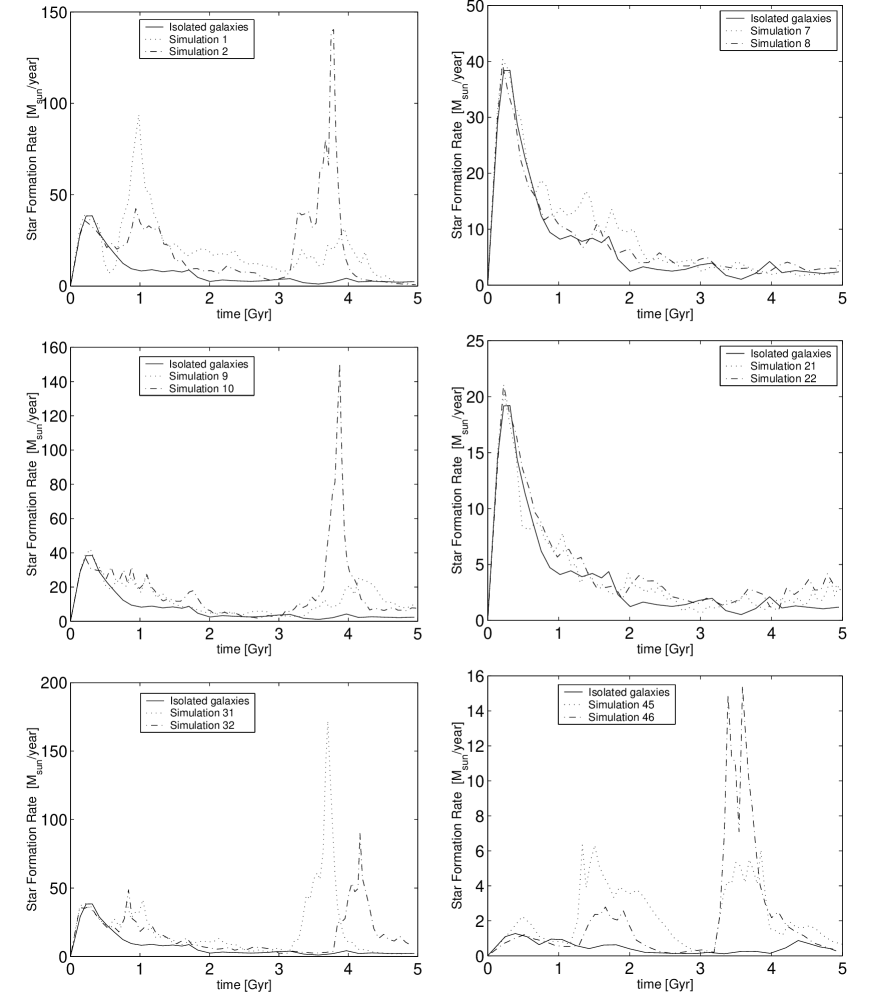
Figure 6: Evolution of the SFRs for several simulations (see Tables 3 and 4). Simulation 1 and 2 show the evolution of the SFRs if the minimum separation is increased. If the minimum separation is increased from 40 to 50 kpc (simulation 7 and 8) the SFRs do not change. In simulation 9 and 10 the big difference between two spatial alignments on the evolution of the SFRs is shown. If one of the interacting galaxies has 10 times less mass and does not form stars by its own (simulation 21 and 22) the overall SFR does not change in comparison to the isolated systems. In simulation 45 and 46 the maximum enhancement of the ISFR of all simulations occurs.

6.2 Collisions between model galaxies A and B

The involved galaxies A and B have a mass ratio of 8:1, see Table 1. The ISFR for the collisions between the model galaxies A and B show that there is only an average increase of by a factor of 1.21 in comparison to the ISFR of the two isolated model galaxies A and B. For collisions between A and B all ISFR are given in units of $\int_{t=0Gyr}^{t=5Gyr}SFR_{A}(t)dt+\int_{t=0Gyr}^{t=5Gyr}SFR_{B}(t)dt\approx 2.2\times 10^{9}$M_☉. Note that the ISFR of the isolated model galaxy B is below 0.5% of the ISFR of the isolated model galaxy A and therefore negligible. Figure 6 shows the evolution of the SFRs of simulations 21 and 22 (see Table 3 for details). As galaxy A has about 8 times more gas than galaxy B the collisions do not increase the ISFR like collisions between two model galaxies A. The SFR of model galaxy A yields therefore the major contribution to the ISFR of simulations 17-28. This leads to the conclusion that a merger of a gas-poor galaxy with a large galaxy like model galaxy A does not lead to a large increase of the SFR. The major effect that we see in our simulations between model galaxy A and B is the redistribution of gaseous and stellar matter in huge spaces around the interacting system. In section 8 this result will be presented in detail.

6.3 Collisions between model galaxies A and C

Simulations 29-44 each involve one system with and one without a bulge (model galaxy A and C). The chosen bulge properties, see Table 1, do not dramatically influence the evolution of the SFRs. Comparing the evolution of the SFRs of the isolated galaxy A (without bulge) and isolated galaxy C (with bulge) does not yield a significant difference, see Fig. 3. ISFR are again given in units of $\int_{t=0Gyr}^{t=5Gyr}SFR_{A}(t)dt+\int_{t=0Gyr}^{t=5Gyr}SFR_{C}(t)dt=4.5\times 10^{9}$M_☉, see Fig. 2. The results show approximately the same behavior as the results of simulations 1-16 (collisions between two model galaxies A). In Fig. 6 the SFRs of simulations 31 and 32 are presented as an example. The decrease of the ISFR by increasing the minimum separation is nearly identical to that of simulations 1-8.

6.4 Collisions between model galaxies B

Collisions between two model galaxies B show the strongest enhancement of ISFR. The maximum enhancement is 4.76 times higher than for the isolated model galaxies. Note that model galaxy B is chosen in such a way that the isolated galaxy show hardly any star formation, see Fig. 3. In case of close interaction the gas can exceed locally the defined threshold for star formation and therefore a dramatic increase of the SFR occurs. Similar to all other simulations, simulations 45,46,47 and 48 show a decrease of the ISFR with increasing minimum separation. Simulation 48 (minimum separation 50 kpc) even results in a decrease of 4% of the ISFR in comparison to the isolated model galaxies. Two isolated model galaxies B form $2.8\times 10^{8}$M_☉ of stars in 5 Gyr. In Fig. 6 the evolution of the SFRs of simulations 45 and 46 are shown as an example.
It is important to point out that interaction of small spiral galaxies can produce strong star formation in comparison to the isolated systems and therefore make them easily observable. They might be good tracers for the frequency of galaxy-galaxy interaction in the distant universe.

7 The gas to star transformation efficiency

Different simulations show different star formation rates and ISFR, therefore they are more or less efficient in transforming gas into stellar matter. The ISFR can be dominated by an extreme starburst-like event for a short duration (several million years) or a long term low enhancement of SFR due to interaction. As observers measure quantities like gas mass or stellar mass/luminosities of a galaxy in a certain evolutionary state of a galaxy, the knowledge of the gas/stellar ratios provides a crucial link between observation and theory. Therefore we elaborate in this section purely on the gas/stellar mass ratios of our simulations.

7.1 Collisions between model galaxies A

For all simulations the ratio of gaseous matter and stellar matter at certain timesteps were calculated. In Table 3 the gas/stellar mass ratios for simulations 1-16 are given. The ratios are always given at the beginning of each simulation (t=0 Gyr), at t=2 Gyr, t=3 Gyr and at t=5 Gyr (end of all simulations). The timesteps were chosen in such a way that they correspond to shortly after the first encounter, shortly before the second encounter and shortly after the second encounter. Except for simulations 7 and 8 all collisions between two model galaxies A end up in a single elliptical galaxy, i.e. they merge. Simulations 7 and 8 do not merge within the simulation time of 5 Gyr, they are just fly-bys with only one encounter. The highest efficiency in converting gaseous matter into stars are found in simulations 1-5. Simulation 16, a counter-rotating collision, shows less efficiency in gaseous to stellar matter conversion than simulation 2, the co-rotating encounter with the identical interaction geometry. Figure 7 shows the ratios of gaseous to stellar matter for simulations 1-8 (increasing minimum separation) for different times. At the beginning of the simulations, 25% of all galaxies’ total disk matter is gas. The efficiency of gaseous to stellar mass conversion follows a nearly linear behavior for simulations 1-8 after the first encounter. The best linear fit for the efficiency after the first encounter is

$$e(r)=0.94\times 10^{-3}\,r+0.15$$ (9)

where $e$ is the ratio of gaseous to stellar matter and r is the minimum separation in kpc. The small slope of $0.94\times 10^{-3}(\textrm{kpc})^{-1}$ shows that there is no strong dependence of $e$ on the minimum separation after the first encounter in our model. This changes dramatically after the second encounter (t=5 Gyr). For simulations 1-4 there is the same, nearly constant, behaviour of $e$. This results from the fact, that for a minimum separation above 40 kpc no merger occurs within the simulation time. For simulations 1-8 we conclude:

• a minimum separation below 20 kpc ($\sim 6\times$R_d) results in an efficiency, which scales nearly linear with r (the minimum separation). This holds for the first and the second encounter. The slope is very flat, therefore no strong dependence is found.

• for minimum separations above 40 kpc there is only one encounter over the whole simulation time of 5 Gyr. Therefore no enhanced star formation due to galaxy-galaxy interaction occurs.

• if the minimum separation is below $\sim 6\times$R_d the quotient $e$ is almost the same for the first and the second encounter, i.e. $\sim$40% of the gas is converted into stars at each collision.

Figure 7: Gas/stellar mass ratio for simulations 1-8 at simulation times 0,2,3 and 5 Gyr

Figure 8 shows the gas to stellar ratios for simulations 2,9,13 and 16 (increasing $\Phi$ for one member of the system). If $\Phi_{2}$ is increased to values of about 90^∘ we find a decrease of the ISFR. If we go beyond $90^{\circ}$ the ISFR increases and therefore the ratios of gaseous to stellar matter decreases. Simulations 2 and 16 show different ratios, this leads to the conclusion that a co-rotating encounter has a higher ISFR than a counter-rotating one. This can be seen in almost all co-rotating counter-rotating simulations, see Table 3. Only simulations 11 and 12 do not comply with this pattern. The results show in addition a greater dependence of the conversion of gaseous into stellar matter on $\Phi_{2}$ after the second encounter (see Fig. 8). Simulations with $45^{\circ}<\Phi_{2}<90^{\circ}$ do have a lower ISFR after the first encounter, which increases by a factor of 2 after the second encounter.

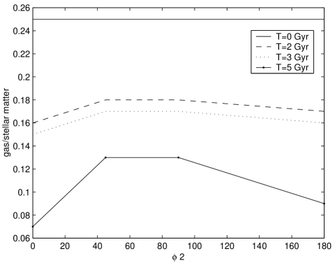
Figure 8: Gas/stellar mass ratio for simulations with increasing $\Phi_{2}$ at simulation times 0,2,3 and 5 Gyr

7.2 Collisions between model galaxies A and B

Simulations 17-28, interaction between model galaxy A and B, do not show a significant difference to the isolated systems. This is due to the fact that the less massive partner in the interacting system has not enough gaseous and stellar matter to disturb the normal evolution of the more massive partner (model galaxy A). However, the smaller partner of the interacting system redistributes the gas and stellar components of both galaxies up to very large distances (several hundred kpc) from the centre of baryonic mass. The next section will go into more details on that. Table 3 lists all the numbers.

7.3 Collisions between model galaxies A and C

The introduction of a spiral galaxy with a bulge (model galaxy C) does not change the efficiency of converting gaseous into stellar matter dramatically. Only at very small minimal separations ($<5$ kpc) the bulge seems to decrease the efficiency, see Table 4. The best linear fit for the efficiency after the first encounter is

$$e(r)=0.76\times 10^{-3}\,r+0.16$$ (10)

where $e$ is the ratio of gaseous and stellar matter and r is the minimum separation in kpc. The difference to equation (9) is very small. After the second encounter the efficiency for transferring gaseous into stellar matter shows the same dependencies on the minimum separation as in simulations 1-8.
Changes of $\Phi_{2}$ show the same behavior as collisions between two model galaxies A. Again the decrease of the efficiency to convert gaseous matter into stellar matter for collisions with $45^{\circ}<\Phi_{2}<90^{\circ}$ can be seen in Fig. 10.

Figure 9: Gas/stellar mass ratio for simulations 29-36 at simulation times 0,2,3 and 5 Gyr

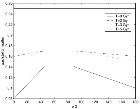
Figure 10: Gas/stellar mass ratio for simulations with increasing $\Phi_{2}$ at simulation time 0,2,3 and 5 Gyr

7.4 Collisions between model galaxies B

As a consequence of the low mass ($\sim\frac{1}{8}$ of model galaxy A and C) the disk scale length R_d for the undisturbed galaxy B is 2.25 $h^{-1}$ kpc. For this reason the efficiency for converting gaseous into stellar matter decreases with increasing minimum separation r very fast (see Fig. 11). For r $>$ 25 kpc almost no enhancement of the ISFR is observable. A close encounter $0<$r$<$5 kpc gives almost the same relative efficiency in converting gas to stellar matter as collisions between two model galaxies A or between galaxies A and C do.

In contrast to that changes of $\Phi_{2}$ result in different efficiencies than the collisions between two model galaxies A (respectively galaxies A and C), see Fig. 12. After the first encounter (t=2 Gyr) no significant change of the efficiency can be seen, but at the end of the simulation time (t=5 Gyr) the efficiency decreases rapidly with increasing $\Phi_{2}$. It seems that a merger of counterrotating model galaxies B does not cause an enhancement of the star formation after the second encounter. The best efficiency is given in the edge on collisions, $\Phi_{2}$=0, with a 2 times higher efficiency after the first encounter than after the second one.

Figure 11: Gas/stellar mass ratio for simulations 45-48 at simulation times 0,2,3 and 5 Gyr

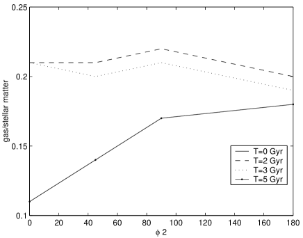
Figure 12: Gas/stellar mass ratio for simulations with increasing $\Phi_{2}$ at simulation times 0,2,3 and 5 Gyr

8 Spatial distribution of gas and stars

New observations and N-body/hydrodynamic simulations do give evidence for an intra-cluster stellar population (ICSP) (Arnaboldi et al. 2003; Murante et al. 2004). Arnaboldi et al. (2003) claim that 10% - 40% of all stars in a galaxy cluster are members of the ICSP. As stars are the hatchery of metals, the ICSP enriches the intra-cluster medium (ICM) directly with metals and energy, see Domainko et al. (2004) and references therein.
It is well known that galaxy-galaxy interactions can enrich the ICM due to strong galactic winds (De Young 1978). Our simulations show beside that another direct enrichment mechanism: vast spatial gaseous and stellar matter distributions as a consequence of galaxy collisions. In Tables 3 and 4 we list the radii within which 80% of the gaseous and stellar matter reside after t=5 Gyr for all carried out simulations. The cut off radii are determined in such way, that in annuli with increasing radii around the centre of mass each particle type (stellar, gaseous and newly formed stars) was integrated. If the sum of a component exceeds 80% of the overall sum of the component, the radius was taken as the cutoff radius (see Fig. 13).

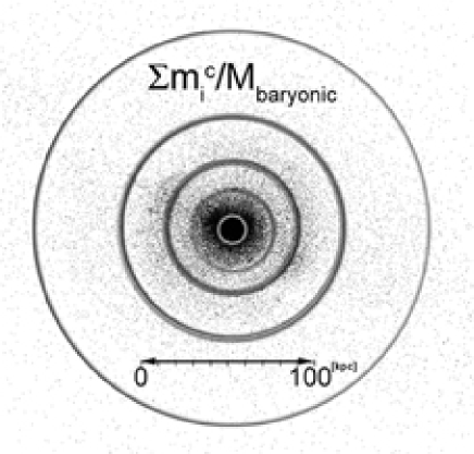
Figure 13: Determination of mass profiles. The rings are centred around the centre of mass of baryonic matter. In each ring the sum over each particle type (stellar, gaseous and newly formed stars) is divided by the total baryonic mass.

The total baryonic masses for the simulations are listed in Table 5.

Table 5: Total baryonic masses for all simulations

	Total baryonic mass
Simulation	[$1\times 10^{10}h^{-1}M_{\sun}$]
1-16	9.5240
17-28	5.3573
29-44	11.9050
45-56	1.1905

Figures 15-17 show the mass profiles for the isolated systems A,B, and C at t=5 Gyr. In comparison to the mass profiles of the interacting systems the profiles are very flat in the innermost 3 kpc and they do not reach as wide into the intergalactic space as the interacting system (see Fig. 19). In the mass profiles of the isolated model galaxies A and B there are kinks at 40 kpc and 30 kpc in the gas component, which coincide with the edges of the stellar disks. This feature can be found in the interacting systems as well (e.g. simulation 39). It marks the transition between cold and hot gas (see Fig. 18).
At first sight it is striking that in collisions A-A, A-C and B-B (all equal mass mergers), the stars are finally more widely spread in space than the gaseous matter components. The non-equal mass mergers (simulations 17-28) on the other hand show the gaseous matter to be almost always by a factor 2 more extended in space than the stellar component. The maximum for the 80% gaseous matter cut off radius can be found in simulation 25 within 20.85 kpc. Figure 19 gives the mass profiles for several simulations. The masses are always given as ratios between mass of the component or total baryonic mass in a ring with radius r_i-r_i-1 and the total baryonic mass of the whole system. Whereas simulations 1-16 (collisions A-A) do have a steeper gradient in their mass profiles within a radius of about 10 kpc, collisions between non-equal mass mergers (simulations 17-28) show flat gradients in this range (see Fig. 19, simulations 1,6,10,18 and 26).

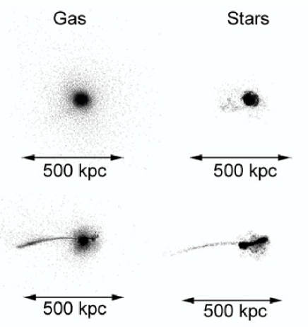
Figure 14: Gas and mass distributions of simulation 13 (upper panel) and simulation 25 (lower panel) at t=5 Gyr.

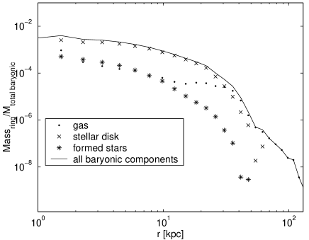
Figure 15: Mass profiles of the baryonic components of the isolated model galaxy A as a function of radius. The masses are given in ratios of each component to the total baryonic mass of the whole system. The binning geometry is given in Fig. 13. The centre of the binning is the centre of mass of the baryonic component. The profiles are given for the last timestep in our simulation (t=5 Gyr).

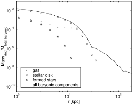
Figure 16: Same as Fig. 15 for model galaxy B

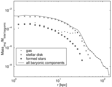
Figure 17: Same as Fig. 15 for model galaxy C

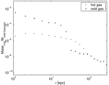
Figure 18: Mass profiles of the hot and cold gas of the isolated model galaxy B as a function of radius. The masses are given in ratios of each component to the total baryonic mass of the whole system. The binning is the same as in Fig. 15. The profiles are given for the last timestep in our simulation (t=5 Gyr).

Simulations 18 and 23-27 show distinct baryonic mass concentrations at r$\sim$100 kpc (see Fig. 19, simulations 18 and 26 for an example). In Fig. 14 the gaseous and stellar matter distributions of simulations 13 and 25 are shown. Simulation 25 shows the remnant of model galaxy B at about this distance of the centre of mass. In addition a huge tail of gas and stars reaching nearly 500 kpc into the surrounding space can be seen. The corresponding mass profiles, Fig. 19 (simulations 18 and 26) show the same features at large radii. Note that for r$>$200 kpc the stellar component decreases dramatically in comparison to the gaseous one. In contrast simulations 18, 22, 25, 26 and 27 show nearly the same mass densities of gas and stellar matter up to 1 Mpc. If we compare the distinct mass concentrations at r$>$200 kpc in simulations 18, 23, 24, 25, 26 and 27 there is a factor of about ten more stellar than gaseous matter. It seems that the passage of the smaller member (model galaxy B) has stripped off nearly all of its gas. Additionally the gas of model galaxy A has been vastly distributed, see Fig. 14 lower panel. The equal mass collisions (simulation 1-16) have common trends in the spatial distribution of the different components. In the innermost circles within radii $<$ 100 kpc the stellar matter is the dominating component. At larger distances of the centre of mass the gaseous matter becomes the dominating component. The newly formed stars are more concentrated near the centre of baryonic mass. The same behaviour can be found in simulations 29-44 (collisions between model galaxies A and C). Collisions between model galaxies B show a similar distribution of baryonic matter. In Fig. 19 simulations 51 and 52 the gaseous component dominates at radii above 100 kpc. The newly formed stars are concentrated in a 10-20 kpc ring around the baryonic center. In simulation 50 stars are formed even at higher radii than the stellar disk reaches. At a distance of 200 kpc from the centre a surface mass density of $\sim$1M_☉ for newly formed stars can be found (see Fig. 19).

Table 6: Radii containing 80% of the mass of the baryonic components. Col. 1: 80% gas mass within radius [kpc] ; Col. 1: 80% stellar mass within radius [kpc] ; Col. 1: 80% newly formed stars within radius [kpc]

	C 1	C2	C3
galaxy A	3.25	3.25	1.53
galaxy B	0.57	1.11	0.57
galaxy C	5.89	4.79	3.02

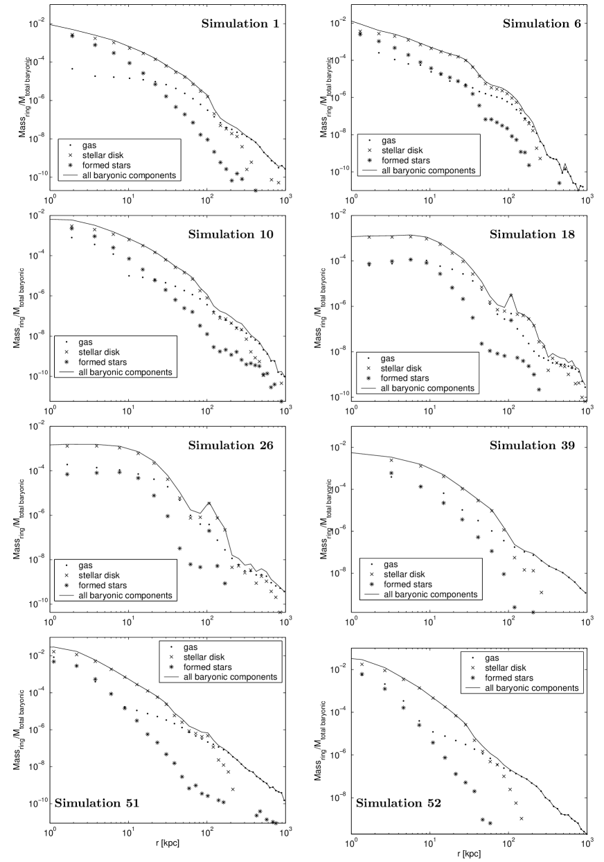
Figure 19: Mass profiles of the baryonic components of the interacting system as a function of the radius. The masses are given in ratios of each component to the total baryonic mass of the whole system. The binning geometry is given in Fig. 13. The center of the binning is the center of mass of the baryonic components. The profiles are given for the last timestep in our simulation (t=5 Gyr).

8.1 The difference between galactic winds and kinetic mass distribution

In Fig. 20 the gas particles for the isolated model galaxy A after 5 Gyr evolution are shown. The image displays the galaxy edge-on in order to see the gas particles above and below the disk due to galactic winds in the lower panel and the absence of gas outside the disk in the upper panel in the case without. In Table 6 the cut off radii of the different components, i.e. gaseous and stellar matter are given. A comparison of the cut off radii of the different components (gaseous matter, stars and newly formed stars) of the interacting systems (see Tables 3 and 4, Col. 18, 19 and 20) with the cut off radii of the isolated systems show no common trend. E.g. the gaseous matter of simulations 1-16 is not widely distributed in space, as in the isolated model galaxy A. Only simulations 1,9 and 13 do not follow that trend and show larger cut off radii. The reason is that the interacting systems do convert much more gas into stars than the isolated ones. Therefore over the simulation time more gas can be expelled by galactic winds in the case of the isolated galaxy. It is important to mention that the interaction between galaxies is a highly dynamic process. At different simulation times of the interacting systems the gaseous matter is distributed over the intergalactic space in form of tidal tails and bridges.

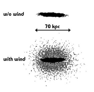
Figure 20: Isolated galaxies after 5 Gyr of evolution with and without wind routine switched on. Only the gas is shown edge on.

As mentioned earlier, simulations 17-28 (interactions between model galaxy A and B) show different results. Due to the mass difference of the interacting systems (1:8) the gaseous matter of the more massive interaction partner is thrown off by the less massive galaxy as it travels through the gaseous disk of its massive partner. A second mechanism is that model galaxy B strips off almost all its gas as a consequence of the first encounter with the other galaxie’s disk.
To investigate the dependence of the mass profile on galactic winds, we did galaxy collisions with and without galactic winds switched on. One major result of our study is, that for our mergers the -kinetic- spreading of gaseous matter is much more efficient than the mass loss due to galactic winds. If the galaxies were isolated, galactic winds can enrich several tens of kpc of the surrounding intergalactic and intra-cluster medium very efficient, see Fig. 20. In Fig. 21 the gas-mass profiles for one merger simulation with and without winds are shown. In the outer parts of the merger, r $>$ 30 kpc, the winds do not change the result. Therefore direct -kinetic- spreading is the dominating process in the outer parts of the merger remnant. Only in the inner parts the winds do change the gas-mass profiles.

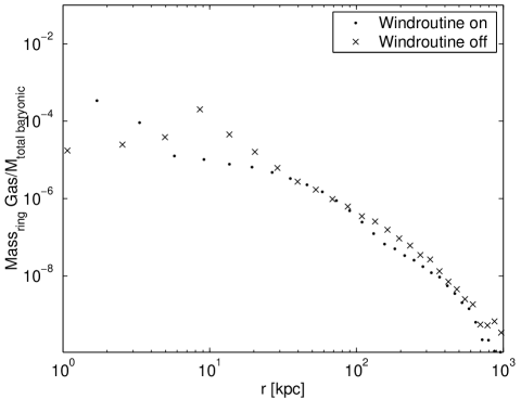
Figure 21: Mass profiles for two simulations (Simulation 2, see Table 3), with wind routine switched on and off.

9 Conclusions and discussion

We present combined N-body/hydrodynamic simulations of interacting spiral galaxies in order to investigate the overall star formation and spatial distribution of baryonic matter due to different encounter geometries and galaxy masses. We performed 56 simulations with average mass resolutions of $1.4\times 10^{5}$ M_☉, $1.1\times 10^{6}$ M_☉ and $9.5\times 10^{5}$ M_☉ per particle. See Table 2 for details on the resolutions. The main results of our simulations are:

1. The simulated interacting disk galaxies show an enhancement of the ISFR of factors up to 5 and on average of a factor 2 in comparison to isolated, undisturbed galaxies. This can be explained in terms of duration and gas content of the interacting system. As in Fig. 6 shown for some simulations the duration of enhanced star formation is very short in comparison to the quiescence star forming epochs. Of course this depends on the relative velocities of the interacting systems. If the velocities would be higher, like in centers of galaxy clusters, the interacting times would be shorter and therefore the disturbances lower and the ISFRs are not so enhanced. The result here holds only, if the relative velocities for the interacting systems are the same.

2. There is a strong dependence of the integrated star formation rate (ISFR) on the minimum separation of the encounter. The enhancement of the star formation scales linearly with a flat slope ($\sim\!\!\!1\!\times 10^{-3}$ kpc^-1) after the first encounter. If the minimum separation is larger than $\sim\!5\times$ the disk scale length R_d at the first encounter the second encounter does not provide an enhancement in the star formation.This is due the fact, that the second encounter does not occur within the simulation time. As the galaxies would have their own SFR over longer periods the second encounter would not have as much gas left as in the case of minimum separation less than $5\times$R_d encounters. Therefore the enhancement would be lower. It is important to note that this result holds only for our chosen parameters, therefore more investigation would be needed to state a more global conclusion.

3. Counter-rotating interacting systems do not always have a lower or higher ISFR in comparison to co-rotating systems. It depends on the spatial alignment of the interacting galaxies. If they interact edge-on, co-rotation does show a $\sim\!\!10$% higher ISFR. On the other hand face-on collisions in general show larger (on average 100%) enhancements of the ISFR for the counter-rotating case. This indicates that the duration of interaction plays an important role, besides the geometry. In the case of face-on interactions the first encounter is very short in comparison to the edge-on interaction. Therefore the short interaction times in the counter-rotating case does provide more disturbances as the co-rotating case.

4. Collisions between model galaxy A (Milky Way type spiral galaxy) and B (tiny spiral galaxy) do not show a significant enhancement of the ISFR. On average 21% more stars are formed than in the isolated systems. As the mass ratio is 1:8 and the disk scale length of model galaxy B is only half the size of model galaxy A, those encounters do not provide as much disturbances in the gaseous disks, as the collisions between model large model galaxies. In addition the relative velocities of the smaller members are higher as in the equal mass merger, which results in shorter interaction times.

5. The mass profiles show that equal mass mergers do not distribute stellar and gaseous matter as far as the non-equal mass mergers. The cut off radii containing 80% mass of the stellar and gaseous components are the largest for collisions between model galaxies A and B (mass ratio 8:1).

Concluding we find that galaxy-galaxy interactions enrich the intergalactic medium in two different processes: indirectly by galactic winds and directly by redistributing gaseous and stellar matter into huge volumes by interaction. If the interacting galaxies have equal mass the galactic winds are the dominating mechanism. But if the interacting system consists of galaxies with a mass ratio of the order of 1:8, the direct process is the dominating one. It is likely that the intergalactic medium is highly enriched by this direct mechanism.

References

- (1) Arnaboldi, M., Freeman, K. C., Okamura, S., et al. 2003, AJ, 125, 514
- (2) Bell, E. F., et al., 2004, APJ, 608, 752
- (3) Breitschwerdt, D., McKenzie, J.F., Völk, H.J., 1991, A&A 245, 79
- (4) Bushouse, H. A., 1987, ApJ 320, 49
- (5) Colina, J., Lipari, S. & Macchetto, 1991, AJ 379, 113
- (6) Cox, T. J.,Primack, J., Jonsson, P., Somerville, R., 2004, ApJ 607, L87
- (7) De Lucia, G., Kauffmann, G., & White, S. D. M., 2004, MNRAS, 349, 1101
- (8) De Young, D. S., 1978, ApJ 223, 47
- (9) Domainko, W., Gitti, M, Schindler, S., Kapferer, W., 2004, A&A, 425, L21
- (10) Duc, P. A., Brinks, E., Springel, V., Pichardo, B., Weilbacher, P., Mirabel, I. F., 2000, ApJ 120, 1238
- (11) Fukazawa Y., Kawano N., Kawashima K., 2004, ApJ 606, L109
- (12) Furusho T., Yamasaki N.Y., Ohashi T., 2003, ApJ 596, 181
- (13) Gnedin, N. Y., 1998, MNRAS 294, 407
- (14) Gunn, J. E., Gott, J. R. III, 1972, ApJ 176, 1
- (15) Kantz, N., Weinberg, D. H., Hernquist, L., 1996, ApJS 105, 19
- (16) Kauffmann, G., White, S. D. M., Heckman, T. M., Ménard, B., Brinchmann, J., Charlot, S., Tremonti, C., & Brinkmann, J., 2004, MNRAS, 353, 713
- (17) Martin, C.L., 1999, ApJ 513, 156
- (18) McKee, C. F., Ostriker, J. P., 1977, ApJ 218, 148
- (19) Mihos, J. C., Dubinski, J., Hernquist, L., 1998, ApJ 494, 183
- (20) Mo, H. J., Mao, S., White, S. D. M., 1998, MNRAS 295, 319
- (21) Murante, G., Arnaboldi, M., Gerhard, O., Borgani, S., Cheng, L. M., Diaferio, A., Dolag, K., Moscardini, L., Tormen, G., Tornatore, L., Tozzi, P., 2004, ApJ 607, L83
- (22) Morganti, R., Sadler, E. M., Oosterloo, T., Pizzella, A., & Bertola, F., 1997, AJ, 113, 937
- (23) Rix, H. W., Barden, M.; Beckwith, S. V. Wet al., 2004, APJS, 152, 163
- (24) Sanders J.S., Fabian A.C., Allen S., Schmidt R.W., 2004, MNRAS 349, 952
- (25) Schmidt R.W., Fabian A.C., Sanders J.S., 2002 MNRAS 337, 71
- (26) Springel, V., Yoshida, N., White, S. D. M., 2001, New Astronomy, 6, 79
- (27) Springel, V., Hernquist, L., 2002, MNRAS, 333, 649
- (28) Springel, V., Hernquist, L., 2003, MNRAS, 339, 289
- (29) Springel, V., Di Matteo, T., Hernquist, L., astro-ph/0411108
- (30) Springel, V., Di Matteo, T., & Hernquist, L., 2005, ApJ, 620, L79
- (31) Springel, V., & Hernquist, L., 2005, ApJ, 622, L9
- (32) Stocke, J. T., 1978, Astron. J. 83, 348
- (33) Sulentic, J. W., 1976, Astrophys. J. Suppl. 32, 171
- (34) Tamura, T., Kaastra, J. S., den Herder, J. W. A., Bleeker, J. A. M., Peterson, J. R., 2004, A&A, 420, 135
- (35) Tornatore, L., Borgani, S., Matteucci, F., Recchi, S., & Tozzi, P., 2004, MNRAS, 349, L19