Differential Emission Measure Determination of Collisionally Ionized Plasma: II. Application to Hot Stars

Abstract

In a previous paper we have described a technique to derive constraints on the differential emission measure (DEM) distribution, a measure of the temperature distribution, of collisionally ionized hot plasmas from their X-ray emission line spectra. We apply this technique to the Chandra/HETG spectra of all of the nine hot stars available to us at the time this project was initiated. We find that DEM distributions of six of the seven O stars in our sample are very similar but that $\theta^{1}$ Ori C has an X-ray spectrum characterized by higher temperatures. The DEM distributions of both of B stars in our sample have lower magnitudes than those of the O stars and one, $\tau$ Sco, is characterized by higher temperatures than the other, $\beta$ Cru. These results confirm previous work in which high temperatures have been found for $\theta^{1}$ Ori C and $\tau$ Sco and taken as evidence for channeling of the wind in magnetic fields, the existence of which are related to the stars’ youth. Our results demonstrate the utility of our method for deriving temperature information for large samples of X-ray emission line spectra.

1 Introduction

In hot stars, X-rays are emitted by gas heated in shocks in the wind. In most cases, these shocks are thought to result from an instability inherent in the mechanism which drives the wind: absorption of stellar UV radiation in line transitions. In some cases, however, other physical processes may play a role in the heating of gas to X-ray emitting temperatures. For example, in very young hot stars, channeling of the wind by magnetic fields may play a strong role in heating the wind (e.g., ud-Doula & Owocki, 2002). Among the evidence that X-ray emission from some hot stars may be due to a mechanism other than the instability of the radiative driving mechanism, is the fact that the X-ray spectra of some hot stars are characteristic of emission by plasma of higher temperature than others.

Line emission from hot plasmas is highly sensitive to temperature. Therefore, insofar as theories of hot star winds make predictions for the temperature of X-ray emitting plasmas in them, high-resolution X-ray spectroscopy offers a powerful method with which to test those theories. However, there are two obstacles in using high-resolution spectroscopy to study the winds of hot stars. First, in most hot stars, the winds from which the X-ray emission arises have velocities in excess of 1000 km s^-1. Owing to this fact, X-ray emission lines are broadened and blended, making it difficult or impossible to measure fluxes of many emission lines (e.g., Cassinelli et al., 2001; Kahn et al., 2001; Schulz et al., 2003). Second, the theory of hot star winds is not sufficiently developed to the point where detailed predictions for X-ray emission line spectra can be made for direct comparison with observations.

While there are open questions regarding the origin of the X-ray emitting plasma in hot stars, it is well established that the emitting plasma in hot stars is in collisional ionization equilibrium (CIE, see, e.g., Paerels & Kahn 2003). In a previous paper (Wojdowski & Schulz, 2004, hereafter Paper I), we have described a method for measuring the differential emission measure (DEM) distribution, a measure of the temperature distribution of a hot, optically thin plasma in collisional ionization equilibrium (CIE). In this method, a number of templates, each of which contains all of the emission lines of a single ion, are fit to an observed high-resolution spectrum. The best-fit normalization for each of these templates then provides a measure of the product of the elemental abundance and a weighted average of the DEM distribution over the range where the ion emits. These measurements may then be plotted in a way that may be described as a one-dimensional “image” of the DEM distribution. This method is well suited to the study of hot stars because the use of templates makes use of the information available from line blends and because it does not require that assumptions about the form of the DEM distribution be made.

In §2 we describe our sample of nine early-type stars which have been observed with Chandra/HETGS, the data, and the application of the method of Paper I to it. In §3 we discuss the implications of our results.

2 Spectral Data Analysis

We obtained the data from the observations of all of the nine bright O stars observed with the Chandra High-Energy Transmission Grating Spectrometer (HETGS). In Table 2, we list these nine stars, the distances and interstellar absorption columns to them that we adopt, and the effective exposure times, Chandra Observation ID numbers, and any references for the Chandra/HETGS observations of them.

For all of the stars in our sample, our analysis proceeds from binned count spectra (PHA files), instrument effective areas and exposure times (ARF files), and wavelength redistribution functions (RMF files). For $\theta^{1}$ Ori C we use the spectral data and instrument response files described by Schulz et al. (2003). For all of the other stars, we use the following procedure. We use spectra extracted as in the standard pipeline processing done by the Chandra X-ray Center. We calculate the appropriate effective area and exposure time for the positive and negative first orders of the the High Energy Grating (HEG) and the Medium Energy Grating (MEG) for each observation using a standard procedure. For each of the two gratings we add the spectra and effective areas for the positive and negative first orders. For those stars observed in two pointings, we add the spectra and exposure times and average the effective areas for the two pointings. In all cases we use the standard redistribution functions. The background expected for these spectra is very low and we make no correction for it.

Table 1: Stars and Data in our Study

				Adopted Values					References
HR #	HD #	Name	Type	Distance	Column Density	Exposure	Obs IDs	Type	Distance	Absorb	Data
				(pc)	($10^{20}$ cm-2)	(sec)
3165	66811string	$\zeta$ Pup	O4I(n)f	450	1.0	68,598	640	24(22)	10,11	15	1
1895	37022string	$\theta^{1}$ Ori C	O4–6p var	450	19string	82,975	3,4	26(22)	15	5	5,6
8281	206267A	$\cdots$	O6.5V((f))	800	30string	72,557	1888,1889	25(22)	12	16	27
2782	57061string	$\tau$ CMa	O9II	1480	5.8	87,095	2525,2526	24(22)	7	7	27
1899	37043string	$\iota$ Ori	O9III	440	2.0	49,917	599,2420	25(22)	13	15	$\cdots$
1852	36486string	$\delta$ Ori A	O9.5II	501	1.5	49,045	639	24(22)	15	15	4
1948	37742string	$\zeta$ Ori A	O9.7Ib	501	3.0	59,640	610	24(22)	15	15	2
6165	149438string	$\tau$ Sco	B0.2V	132	2.7	59,630	638	23	8(3)	15	3
4853	111123string	$\beta$ Cru	B0.5III	110	1.7	74,379	2575	18	8(9)	14	$\cdots$

References. — (1) Cassinelli et al. 2001; (2) Waldron & Cassinelli 2001; (3) Cohen et al. 2003; (4) Miller et al. 2002; (5) Schulz et al. 2000; (6) Schulz et al. 2001, 2003; (7) Moitinho et al. 2001; (8) Perryman et al. 1997; (9) Alcalá et al. 2002; (10) Brandt et al. 1971; (11) Schaerer et al. 1997; (12) Simonson 1968; (13) consistent with Hillenbrand 1997 and references therein; (14) Code et al. 1976; (15) Berghöfer et al. 1996, BSC; (16) Shull & van Steenberg 1985; (18) Hiltner et al. 1969; (22) Maíz-Apellániz et al. 2004; (23) Walborn 1971; (24) Walborn 1972; (25) Walborn 1973; (26) Walborn 1981; (27) Schulz 2003

For each of the nine data sets, we apply the procedure described in Paper I — i.e., we fit the spectra using templates, each of which contains all of the emission lines of an ion. In each of our fits to the stellar data, we use two bremsstrahlung components except in the case of $\tau$ Sco, $\theta^{1}$ Ori C, and $\zeta$ Ori where three are necessary to fit the continuum. In each case, the model spectrum includes neutral, interstellar absorption fixed at the value listed in Table 2. As explained in Paper I, the normalization parameter of each emission line template obtained in the fit implies a constraint on the product of the elemental abundance and a weighted average of the DEM distribution:

$$D_{Z,z}\equiv{}A_{Z}\frac{\int{}_{-\infty}^{\infty}\theta_{Z,z}(T)\mathcal{D}{}(T)d\log{}T}{\int_{-\infty}^{\infty}\theta_{Z,z}(T)d\log{}T}$$ (1)

where $Z$ is the atomic number of the element, $z$ is the charge state, $A$ is the elemental abundance defined relative to solar, $\mathcal{D}{}$ is the differential emission measure distribution, $T$ is temperature, and $\theta$ is the sum of the power functions (described in Paper I) for the lines of the ion. In Figures 1 and 2 we plot $D$ vs. $T_{\rm p}$, where $T_{{\rm p},Z,z}$ is the temperature where the function $\theta_{Z,z}$ peaks. In all of these plots, we use the same temperature range on the horizontal axis as in the plots in Figures 2 and 3 of Paper I and, also as in those figures, the vertical axes span three orders of magnitude. Therefore slopes of lines in these various plots may be compared. As in Paper I, we model the emission lines as Gaussians and allow the centers and widths of all of the Gaussians to vary together. The parameters which describe the centers and widths of the lines are, respectively, $v_{\rm r}$ and $v_{\rm t}$ and we tabulate the best-fit values of these parameters in Table 2. The exact dependence of the model line profiles on these parameters is given in equations 16 and 17 of Paper I. While we have not quantitatively assessed the quality of the fits, it may be seen from the spectral plots that the fits are quite good considering the large number of lines apparent in the data.

As we have described in Paper I, some excited states of some ions are metastable and may undergo further excitation before decaying to ground (pumping) and this leads the luminosities of some emission lines to depend on physical variables other than the DEM distribution. In the vicinity of a hot star, ions in many metastable states are susceptible to excitation by the absorption of UV radiation from the stellar photosphere. As we have also described in Paper I, we account for any line pumping by letting the line ratios in the templates vary as with collisional pumping with one free density parameter for each ion. This approach is somewhat ad hoc. However, the fact that we obtain good fits to the spectra indicates that pumping is well accounted for. Therefore, we do not expect significant errors in our constraints due to line pumping or inaccuracies in our treatment of it.

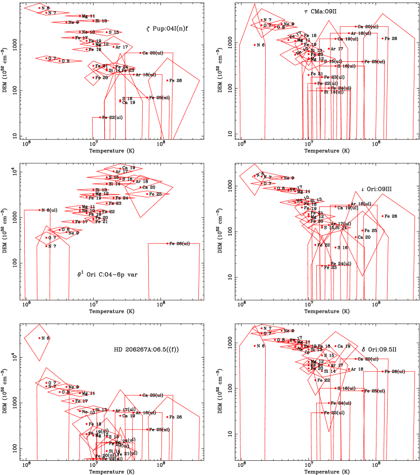
Figure 1: Plots of $D$ as a function of temperature for $\zeta$ Pup, $\theta^{1}$ Ori C, HD 206267A, $\tau$ CMa, $\iota$ Ori, and $\tau$ Sco. The horizontal location of the data points is at the temperature where the ion’s emission peaks. The horizontal extents of the diamonds give the temperature range over which the ions’ emission is significant and the vertical extents of the diamonds give the statistical confidence intervals for the values of $D$. The designation “(ul)” indicates an upper limit.

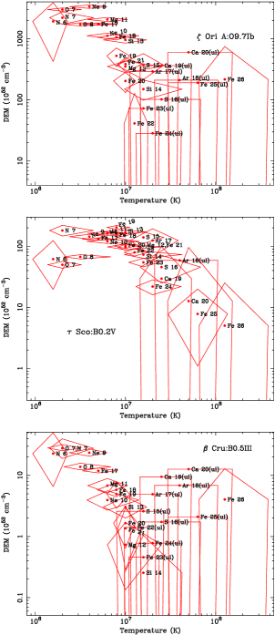
Figure 2: DEM constraints for $\zeta$ Ori A, $\delta$ Ori, and $\beta$ Cru.

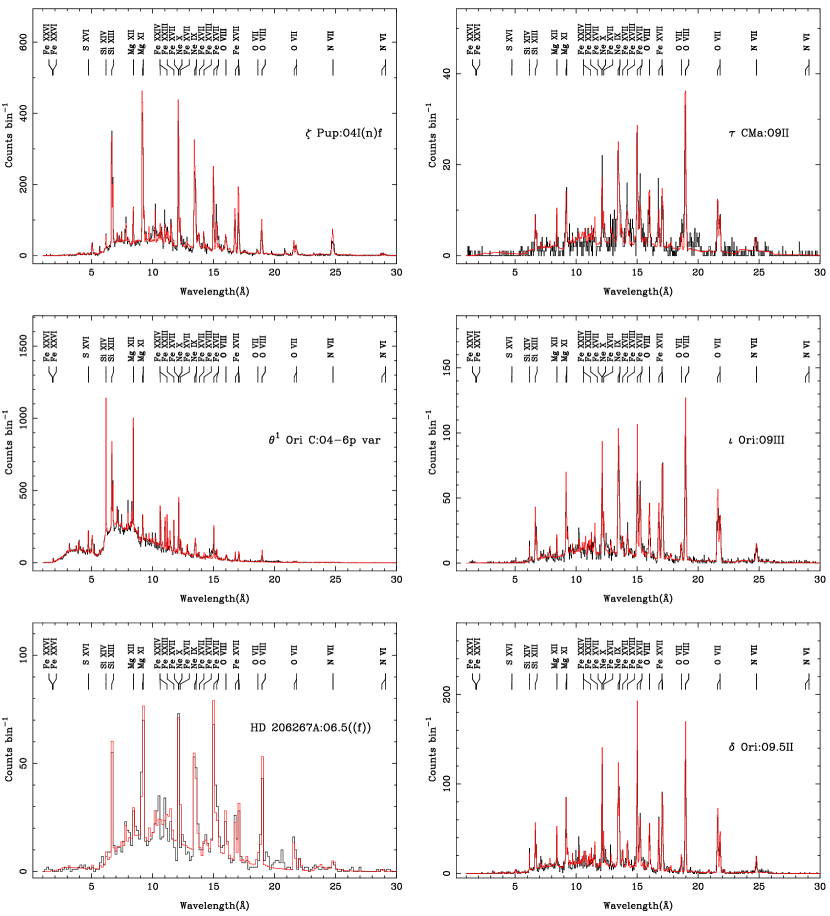
Figure 3: MEG spectral data (black) and best-fit models (red) for $\zeta$ Pup, $\theta^{1}$ Ori C, HD 206267A, $\tau$ CMa, $\iota$ Ori, and $\tau$ Sco. We include a number of line labels though not all of the labeled lines are detected in every spectrum.

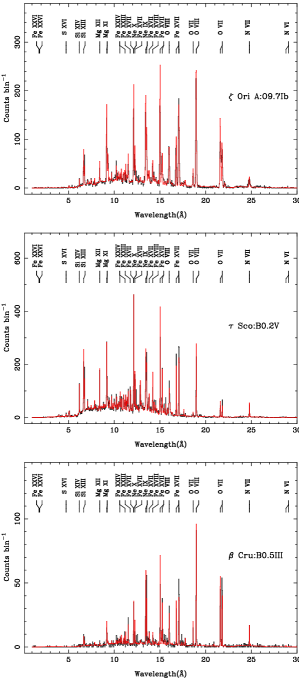
Figure 4: MEG spectral data and best-fit models for $\zeta$ Ori A, $\delta$ Ori, and $\beta$ Cru.

In the plots of $D$ vs. $T_{\rm p}$, for nearly every two ions with close values of $T_{\rm p}$, the corresponding values of $D$ generally appear to be consistent with each other or differ by no more than a factor of two, indicating that the emission line spectrum is consistent with emission from a plasma with solar abundances. One exception to this is the fact that, for $\zeta$ Pup, the values of $D$ for oxygen are approximately an order of magnitude less than the values for ions with similar values of $T_{\rm p}$. A similar result has been obtained by Kahn et al. (2001). The values of $D$ for nitrogen appear to fit better with the rest of the data points than do the values for oxygen. Therefore, it is probably the case that oxygen is underabundant in the wind of $\zeta$ Pup. However, from this analysis alone, it is impossible to exclude a hypothesis in which the DEM distribution of $\zeta$ Pup peaks at approximately $3\times 10^{6}$ K, the abundance of nitrogen is greater than the solar value, and the abundance of oxygen is near the solar value. In addition, there is significant scatter in the data points for $\zeta$ Pup in the temperature range $4\times 10^{6}$–$10^{7}$ K. Some, but not all, of this scatter might be accounted for by an underabundace of iron. For $\tau$ Sco, like $\zeta$ Pup, the values of $D$ for oxygen fall below the values for other ions at nearby temperatures, though not by as much.

Another exception to our results being consistent with solar abundance is $\theta^{1}$ Ori C. For this star, most of the values of $D$ appear to lie on a single curve except for those of the ions Fe XX– XXIV which lie below it by a factor of approximately four. Schulz et al. (2003) fit this spectrum using an explicit parameterized empirical model for the DEM distribution with variable element abundances. The best-fit DEM distribution these authors derive has three peaks at 7.9, 25, and 63 MK and troughs at 13 and 40 MK and vanishes towards temperatures higher and lower than the three peaks. This three-peaked structure is not immediately apparent in our constraints for $\theta^{1}$ Ori C shown in Figure 1. We have explicitly evaluated the right-hand side of equation 1 for the element abundances and DEM distribution of Schulz et al. (2003) and while the values of $D$ for some ions have statistically significant differences, there does not appear to be an overall systematic difference between the values of $D$ obtained by the two methods. In particular, as with the values of $D$ obtained by our method, the triply peaked DEM distribution is also not immediately apparent in the values of $D$ obtained from the abundances and triply peaked DEM distribution of Schulz et al. (2003). This is somewhat puzzling. However, while a triply peaked DEM distribution is not immediately apparent in our results, from a closer look it may be seen how a triply peaked DEM distribution may be found with the method of Schulz et al. (2003). In the method of Schulz et al. (2003), the formula for the quality of fit includes a penalty for variations in the DEM distribution so, if possible, elemental abundances will be adjusted to produce a flat DEM distribution. Variations in the DEM distribution will be found only when lines of the same element require it. Following our values of $D$ for Fe XVII–Fe XXIV, the first peak, the following trough, and the rise to the second peak may be seen. The trough after the second peak may be seen in the drop from Ar XVII to Ar XVIII and from Ca XIX to Ca XX. The rise to the third peak may be seen from the fact that the point for Fe XXV is higher than the one for Fe XXIV.

In order to compare our constraints on the DEM distributions of the stars in our sample with each other, we plot a composite of the nine stars in Figure 5. This figure is constructed as follows. For each star, we ignore those values of $D$ without lower limits. For the case of $\zeta$ Pup we also ignore the values of $D$ for oxygen. Then, for those ions with the same value of $T_{\rm p}$ as given in Table 1 of Paper I, we average the values of $D$ weighting by the inverse square of the uncertainties. The lines connect the averaged values of $D$ for individual stars. Because the method used to construct this figure is ad hoc and because doing so would make the figure harder to read, we do not attempt to include errors in this figure. However, the magnitude of the errors for this figure may be inferred from Figures 1 and 2 and may also be inferred from the jagged curves. The lines for HD 206267A, $\iota$ Ori, $\zeta$ Pup, $\zeta$ Ori A, $\tau$ CMa, and $\delta$ Ori A are very similar and difficult to show together. Therefore, we show the line for $\zeta$ Pup and a filled polygon that encloses the lines for the other five stars. The axes and aspect ratio of this plot are chosen so that slopes in this figure can be compared with Figures 2 and 3 of Paper I and Figures 1 and 2 of this paper.

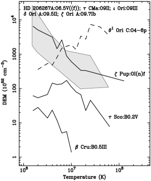
Figure 5: A composite approximate representation of of the DEM constraints we derive for the nine stars. The filled polygon encloses the lines for HD 206267A, $\iota$ Ori, $\zeta$ Pup, $\zeta$ Ori A, $\tau$ CMa, and $\delta$ Ori A which are very similar and difficult to show together. The jagged shape of the curves gives some idea of the magnitude of the error for the DEM constraints. Details of the construction of this figure are given in the text.

With the exceptions of $\tau$ Sco and $\theta^{1}$ Ori C, it may be inferred from these plots that, in the temperature range $10^{6}$–$10^{8.5}$ K, the DEM distributions have peaks at temperatures of a few times $10^{6}$ K and decrease towards higher temperatures. The DEM distribution of $\beta$ Cru, in addition to having a smaller magnitude than the other stars, declines more rapidly towards high temperatures. For $\tau$ Sco, the peak of the DEM distribution and the majority of the emission appear to be at approximately $10^{7}$ K. Most of the emission measure for $\theta^{1}$ Ori C appears to lie near $3\times 10^{7}$ K. In Figures 3 and 4, it may be seen that for many of stars, the points for some or all of the ions Fe XXIV, Fe XXV, and Fe XXVI are higher than those of lower charge states of iron. This suggests the possibility that these DEM distributions increase at temperatures near $10^{8}$ K. However, all of these high temperature points have low statistical significance and it is not possible from this analysis to confirm the presence of any such high temperature increase in the DEM distribution.

We give the best-fit line shifts and widths from our fits in Table 2. If we add the systematic uncertainty of the Chandra HETG absolute wavelength calibration (a few tens of km s^-1) to the tabulated statistical confidence intervals, all of the line shifts we measure are consistent with zero, with the exception of $\zeta$ Pup and the possible exception of $\zeta$ Ori. The blueshift we find for $\zeta$ Pup is consistent with those reported by Kahn et al. (2001) and Cassinelli et al. (2001). The latter authors attribute this blueshift to obscuration of the far side of wind by photoelectric absorption in nearer parts of the wind.

Star	Type	$v_{\rm r}$ (km s-1)	$v_{\rm t}$ (km s-1)
$\zeta$ Pup	O5Iaf	-460$\pm$20	770$\pm$20
$\theta^{1}$ Ori C	O6pe	-29${}^{+15}_{-14}$	326$\pm$18
HD 206267A	O6.5V((f))	-10$\pm$140	1020${}^{+140}_{-130}$
$\zeta$ Ori A	O9Iab	-130$\pm$20	689$\pm$19
$\tau$ CMa	O9Ib	-120${}^{+100}_{-110}$	990${}^{+100}_{-90}$
$\iota$ Ori	O9III	60$\pm$40	930${}^{+40}_{-30}$
$\delta$ Ori A	O9.5II	10$\pm$30	690$\pm$30
$\tau$ Sco	B0V	37$\pm$10	159${}^{+14}_{-15}$
$\beta$ Cru	B0.5III	-12$\pm$19	190$\pm$30

Table 2: Fit Line Shifts and Width Parameters

The blueshift we observe for $\zeta$ Ori A may also be due to this effect. This possibility is discussed by Waldron & Cassinelli (2001).

3 Discussion

We use a method, described in Paper I, to determine the DEM distribution for a sample of nine hot stars which works by fitting entire X-ray spectra. The fact that for all of the nine stars in our sample good spectral fits are obtained suggests that the method is free of significant systematic errors. We find that the magnitudes of the DEM distributions of the two B stars $\tau$ Sco and $\beta$ Cru are much lower than those of the O stars as expected from previous results (e.g., Berghöfer et al., 1996). For all of the stars in our sample except for $\theta^{1}$ Ori C and $\tau$ Sco we find the DEM distributions to be peaked at a temperature of a few times $10^{6}$ K or less, to decline up to several times $10^{7}$ K. Though we cannot confirm it, the DEM distributions of these stars may also increase at temperatures near $10^{8}$ K. In contrast, we find that the peak of the DEM distribution of $\tau$ Sco is near $10^{7}$ K and the peak of the DEM distribution of $\theta^{1}$ Ori C is near $3\times 10^{7}$ K. For those two stars we also find that the emission lines are narrow compared to stars of similar stellar type. High temperatures and narrow lines have previously been found for $\tau$ Sco by Cohen et al. (2003) and for $\theta^{1}$ Ori C by Schulz et al. (2001, 2003) using these same data from Chandra. In both cases, it has been noted that the stars are young and that the high temperatures and narrow lines have been attributed to channeling of the wind in fossil magnetic fields. In this scenario, wind travels up the sides of magnetic loops, then shocks as wind from the two sides of the loop collides. Because the post-shock gas is stationary, narrow lines are predicted. The fact that the post-shock gas is stationary also results in a larger velocity difference between the gas before and after the shock and, therefore, higher temperatures (ud-Doula & Owocki, 2002).

The fact that the X-ray emitting plasma in the wind of $\tau$ Sco is hotter than the X-ray emitting plasma in most stars has been apparent from spectra of much lower resolution (e.g., Cohen, Cassinelli, & MacFarlane, 1997a, b). A hot X-ray emitting plasma has also previously been detected from the Orion Trapezium cluster which contains $\theta^{1}$ Ori C (Yamauchi et al., 1996) though it was not until a high-resolution image was obtained with Chandra by Schulz et al. (2001) that this hot plasma could be conclusively associated with $\theta^{1}$ Ori C. Therefore, our finding that the temperatures of the X-ray emitting plasmas $\theta^{1}$ Ori C and $\tau$ Sco are high is neither a new result of high-resolution spectroscopy nor of our analysis technique. However, as we have shown here, the method described in Paper I is useful in deriving well-defined quantitative constraints on elemental abundances and differential emission measure distributions from high-resolution X-ray spectra and, especially, large samples of high-resolution X-ray spectra. We expect that these results and the results of similar observations and analyses will provide direction for developing theory on X-ray emission in hot stars.

References

- Alcalá et al. (2002) Alcalá, J. M., Covino, E., Melo, C., & Sterzik, M. F. 2002, A&A, 384, 521
- Berghöfer et al. (1996) Berghöfer, T. W., Schmitt, J. H. M. M., & Cassinelli, J. P. 1996, A&AS, 118, 481
- Brandt et al. (1971) Brandt, J. C., Stecher, T. P., Crawford, D. L., & Maran, S. P. 1971, ApJ, 163, L99
- Cassinelli et al. (2001) Cassinelli, J. P., Miller, N. A., Waldron, W. L., MacFarlane, J. J., & Cohen, D. H. 2001, ApJ, 554, L55
- Code et al. (1976) Code, A. D., Bless, R. C., Davis, J., & Brown, R. H. 1976, ApJ, 203, 417
- Cohen et al. (1997a) Cohen, D. H., Cassinelli, J. P., & MacFarlane, J. J. 1997a, ApJ, 487, 867
- Cohen et al. (1997b) Cohen, D. H., Cassinelli, J. P., & Waldron, W. L. 1997b, ApJ, 488, 397
- Cohen et al. (2003) Cohen, D. H., de Messières, G. E., MacFarlane, J. J., Miller, N. A., Cassinelli, J. P., Owocki, S. P., & Liedahl, D. A. 2003, ApJ, 586, 495
- Conti (1972) Conti, P. S. 1972, ApJ, 174, L79
- Hillenbrand (1997) Hillenbrand, L. A. 1997, AJ, 113, 1733
- Hiltner et al. (1969) Hiltner, W. A., Garrison, R. F., & Schild, R. E. 1969, ApJ, 157, 313
- Kahn et al. (2001) Kahn, S. M., Leutenegger, M. A., Cottam, J., Rauw, G., Vreux, J.-M., den Boggende, A. J. F., Mewe, R., & Güdel, M. 2001, A&A, 365, L312
- Maíz-Apellániz et al. (2004) Maíz-Apellániz, J., Walborn, N. R., Galué, H. Á., & Wei, L. H. 2004, ApJS, 151, 103
- Miller et al. (2002) Miller, N. A., Cassinelli, J. P., Waldron, W. L., MacFarlane, J. J., & Cohen, D. H. 2002, ApJ, 577, 951
- Moitinho et al. (2001) Moitinho, A., Alves, J., Huélamo, N., & Lada, C. J. 2001, ApJ, 563, L73
- Paerels & Kahn (2003) Paerels, F. B. S., & Kahn, S. M. 2003, ARA&A, 41, 291
- Perryman et al. (1997) Perryman, M. A. C. et al. 1997, A&A, 323, L49
- Schaerer et al. (1997) Schaerer, D., Schmutz, W., & Grenon, M. 1997, ApJ, 484, L153
- Schulz (2003) Schulz, N. S. 2003, in Revista Mexicana de Astronomia y Astrofisica Conference Series, Vol. 15, 220–222
- Schulz et al. (2001) Schulz, N. S., Canizares, C., Huenemoerder, D., Kastner, J. H., Taylor, S. C., & Bergstrom, E. J. 2001, ApJ, 549, 441
- Schulz et al. (2003) Schulz, N. S., Canizares, C., Huenemoerder, D., & Tibbets, K. 2003, ApJ, 595, 365
- Schulz et al. (2000) Schulz, N. S., Canizares, C. R., Huenemoerder, D., & Lee, J. C. 2000, ApJ, 545, L135
- Shull & van Steenberg (1985) Shull, J. M. & van Steenberg, M. E. 1985, ApJ, 294, 599
- Simonson (1968) Simonson, S. C. I. 1968, ApJ, 154, 923
- ud-Doula & Owocki (2002) ud-Doula, A. & Owocki, S. P. 2002, ApJ, 576, 413
- Walborn (1971) Walborn, N. R. 1971, ApJS, 23, 257
- Walborn (1972) —. 1972, AJ, 77, 312
- Walborn (1973) —. 1973, AJ, 78, 1067
- Walborn (1981) —. 1981, ApJ, 243, L37
- Waldron & Cassinelli (2001) Waldron, W. L. & Cassinelli, J. P. 2001, ApJ, 548, L45
- Wojdowski & Schulz (2004) Wojdowski, P. S. & Schulz, N. S. 2004, ApJ, 616
- Yamauchi et al. (1996) Yamauchi, S., Koyama, K., Sakano, M., & Okada, K. 1996, PASJ, 48, 719