Relativistic Magnetohydrodynamics In Dynamical Spacetimes:
Numerical Methods And Tests

Abstract

Many problems at the forefront of theoretical astrophysics require the treatment of magnetized fluids in dynamical, strongly curved spacetimes. Such problems include the origin of gamma-ray bursts, magnetic braking of differential rotation in nascent neutron stars arising from stellar core collapse or binary neutron star merger, the formation of jets and magnetized disks around newborn black holes, etc. To model these phenomena, all of which involve both general relativity (GR) and magnetohydrodynamics (MHD), we have developed a GRMHD code capable of evolving MHD fluids in dynamical spacetimes. Our code solves the Einstein-Maxwell-MHD system of coupled equations in axisymmetry and in full 3+1 dimensions. We evolve the metric by integrating the BSSN equations, and use a conservative, shock-capturing scheme to evolve the MHD equations. Our code gives accurate results in standard MHD code-test problems, including magnetized shocks and magnetized Bondi flow. To test our code’s ability to evolve the MHD equations in a dynamical spacetime, we study the perturbations of a homogeneous, magnetized fluid excited by a gravitational plane wave, and we find good agreement between the analytic and numerical solutions.

I Introduction

Magnetic fields play a crucial role in determining the evolution of many relativistic objects. In any highly conducting astrophysical plasma, a frozen-in magnetic field can be amplified appreciably by gas compression or shear. Even when an initial seed field is weak, the field can grow in the course of time to significantly influence the gas dynamical behavior of the system. In problems where the self-gravity of the gas can be ignored, simulations can be performed without numerically evolving the spacetime metric. Some accretion problems fall into this category. In many other problems, the effect of the magnetized fluid on the metric cannot be ignored, and the two must be evolved self-consistently. The final fate of many of these relativistic astrophysical systems, and their distinguishing observational signatures, may hinge on the role that magnetic fields play during the evolution. Some of these systems are promising sources of gravitational radiation for detection by laser interferometers such as LIGO, VIRGO, TAMA, GEO and LISA. Some also may be responsible for gamma-ray bursts. Examples of astrophysical scenarios involving strong-field dynamical spacetimes in which MHD effects may play a decisive role include the following:

$\bullet$ The merger of binary neutron stars. The coalescence can lead to the formation of a hypermassive star supported by differential rotation bns_merger ; stu03 . While such a star may be dynamically stable against gravitational collapse and bar formation, the radial stabilization due to differential rotation is likely to be temporary. Magnetic braking and viscosity combine to drive the star to uniform rotation, even if the seed magnetic field and the viscosity are small mag_braking . This process can lead to delayed collapse and massive disk formation dlss04 , accompanied by a delayed gravitational wave burst. MHD-related instabilities in differentially rotating stars might also drive a gamma-ray burst kr98 .

$\bullet$ Core collapse in a supernova. Core collapse may induce differential rotation, even if the rotation of the progenitor at the onset of collapse is only moderately rapid and almost uniform (see, e.g. ccollapse , and references therein). Differential rotation can wind up a frozen-in magnetic field to high values, at which point it may provide a significant source of stress, which could affect the explosion mhd_sn .

$\bullet$ The generation of gamma-ray bursts (GRBs). Short-duration GRBs are thought to result from binary neutron star mergers narayan92 , or tidal disruptions of neutron stars by black holes ruffert99 , or hypergiant flares of ‘magnetars’ associated with the soft gamma-ray repeaters ngpf05 . Long-duration GRBs likely result from the collapse of rotating, massive stars which form black holes (‘collapsars’) macfadyen99 . In current scenarios, the burst is powered by the extraction of rotational energy from the neutron star or black hole, or from the remnant disk material formed around the black hole vlahakis01 . Strong magnetic fields provide a likely mechanism for extracting this energy on the required timescale and driving collimated GRB outflows in the form of relativistic jets meszaros97 . Even if the initial magnetic fields are weak, they can be amplified to the required values by differential motions MRIs .

$\bullet$ Supermassive black hole (SMBH) formation. The origin of the SMBHs observed in galaxies and quasars is one of the great mysteries of contemporary astrophysics. Several hypotheses for the origin of SMBHs involve relativistic, self-gravitating fluids in which magnetic fields can play an important role. It is thought that SMBHs start from smaller initial seed black holes, which grow to supermassive size by a combination of accretion and mergers. The seed black holes might be provided by the collapse of massive ($M\sim 10^{2}M_{\odot}$) Population III stars mr01 . If so, magnetic forces will affect the collapse leading to the formation of these seeds, as well as their growth by accretion gsm04 ; s05 . Another possibility is that SMBHs form directly from the catastrophic collapse of supermassive stars (SMSs) r84 . This collapse will proceed differently, depending on whether the SMS rotates uniformly or differentially ns01 . Magnetic fields and turbulence provide the principle mechanisms that can damp differential rotation in such stars zn71 and thus determine their ultimate fate.

$\bullet$ The r-mode instability in rotating neutron stars. This instability has been proposed as a possible mechanism for limiting the angular velocities in neutron stars and producing observable quasi-periodic gravitational waves r_modes . However, preliminary calculations suggest that if the stellar magnetic field is strong enough, r-mode oscillations will not occur rlms01 . Even if the initial field is weak, fluid motions produced by these oscillations may amplify the magnetic field and eventually distort or suppress the r-modes altogether. (R-modes may also be suppressed by non-linear mode coupling saftw02 or hyperon bulk viscosity jl02 .)

$\bullet$ Massive disk accretion. The importance of magnetic effects on gas accretion onto a black hole is well known. In many cases, the density of the accreting material is small enough that its effect on the spacetime geometry is negligible. Such systems can be studied by evolving the gas on the stationary Kerr spacetime background produced by the central black hole. There are, however, situations in which accretion disks with masses comparable to that of the central black hole can be formed. Examples include the collapse of rapidly rotating stars or supermassive stars ss02 , and neutron star merger (especially when the two neutron stars have unequal masses stu03 ). In these cases, the spacetime is dynamical and Einstein’s equations for the metric must be evolved along with the MHD equations.

In the recent years, numerical codes which evolve the general relativistic MHD equations on fixed Schwarzschild or Kerr black hole spacetimes have been developed by Yokosawa y93 , Koide et al ksk99 , Komissarov k04 , De Villiers and Hawley dVh03 , and Gammie et al HARM . These codes have been used to study the structure of accretion flows onto Kerr black holes mg04 ; dVhk03 , the Blandford-Znajek effect in low-density regions near the hole k04 ; k05 , and the formation of GRB jets myks04 .

In contrast to the above effort, few attempts have been made to simulate relativistic MHD flows in dynamical spacetimes. One major attempt was by Wilson, thirty years ago w75 . He simulated the collapse of a rotating SMS with a frozen-in poloidal magnetic field in axisymmetry using a code which assumed the conformal flatness approximation for the spatial metric. No gravitational radiation is allowed in this approximation. Wilson’s work was generalized by Nakamura, Oohara and Kojima in 1987 nok87 . They studied the effect of poloidal magnetic fields on the collapse of nonrotating SMSs in full GR in axisymmetry. Since the stars are nonrotating, toroidal fields are not generated, which simplifies the calculation. Since then, no other simulations of this kind have been attempted. However, in anticipation of future numerical work, formulations of the coupled Einstein-Maxwell-MHD equations were proposed by Sloan and Smarr ss85 , by Zhang z89 , and by Baumgarte and Shapiro bs03 .

In this paper, we present the first code capable of evolving the Einstein-Maxwell-MHD equations without approximation in both two dimensions (axisymmetry) and three dimensions. Our code is based on the Baumgarte-Shapiro-Shibata-Nakamura (BSSN) formulation of the 3+1 Einstein field equations BSSN . In previous papers, we have evolved the BSSN equations coupled to a perfect fluid dmsb03 , and we have applied our code to simulate stellar collapse and binary neutron star inspiral dmsb03 ; mdsb04 . We then generalized our code to study fluids with shear viscosity dlss04 , and we implemented black hole excision techniques to study the collapse of fluid stars to black holes dsy04 . In this paper, we have completely reformulated the hydrodynamics sector of our code in order to improve its accuracy and shock-handling capability. We have extended the code to allow for a magnetic field frozen into a perfectly conducting fluid in the MHD approximation.

In Sec. II, we present the evolution equations integrated by our code. In Sec. III, we discuss the adopted numerical techniques. We perform a variety of code tests in Sec. IV, including magnetized shocks, a magnetized Bondi accretion flow, and a linear gravitational wave that excites MHD waves.

II Formalism

II.1 Evolution of the gravitational fields

Throughout this paper, Latin indices denote spatial components (1-3) and Greek indices denote spacetime components (0-3). We write the metric in the form

$$ds^{2}=-\alpha^{2}dt^{2}+\gamma_{ij}(dx^{i}+\beta^{i}dt)(dx^{j}+\beta^{j}dt),$$ (1)

where $\alpha$, $\beta^{i}$, and $\gamma_{ij}$ are the lapse, shift, and spatial metric, respectively. The extrinsic curvature $K_{ij}$ is defined by

$$(\partial_{t}-{\mathcal{L}}_{\beta})\gamma_{ij}=-2\alpha K_{ij},$$ (2)

where ${\mathcal{L}}_{\beta}$ is the Lie derivative with respect to $\beta^{i}$. We adopt geometrized units, so that $G=c=1$. We evolve $\gamma_{ij}$ and $K_{ij}$ using the BSSN formulation BSSN . The fundamental variables for BSSN evolution are

$$\phi \equiv {1\over 12}\ln[\det(\gamma_{ij})]\ ,$$ (3)

$$\tilde{\gamma}_{ij} \equiv e^{-4\phi}\gamma_{ij}\ ,$$ (4)

$$K \equiv \gamma^{ij}K_{ij}\ ,$$ (5)

$$\tilde{A}_{ij} \equiv e^{-4\phi}(K_{ij}-{1\over 3}\gamma_{ij}K)\ ,$$ (6)

$$\tilde{\Gamma}^{i} \equiv -\tilde{\gamma}^{ij}{}_{,j}\ .$$ (7)

The evolution and constraint equations for these fields are summarized in BSSN ; dsy04 . In the presence of mass-energy, these evolution equations contain the following source terms:

$$\rho = n_{\alpha}n_{\beta}T^{\alpha\beta}\ ,$$

$$S_{i} = -\gamma_{i\alpha}n_{\beta}T^{\alpha\beta}\ ,$$ (8)

$$S_{ij} = \gamma_{i\alpha}\gamma_{j\beta}T^{\alpha\beta}\ ,$$

where $T^{\alpha\beta}$ is the stress tensor, and $n^{\alpha}=(\alpha^{-1},-\alpha^{-1}\beta^{i})$ is the time-like unit vector normal to the $t=$ constant time slices. Note that, since the electromagnetic fields contribute to $T^{\alpha\beta}$, they will contribute to $\rho$, $S_{i}$, and $S_{ij}$ as shown in Eq. (8).

In order to evolve the 3+1 Einstein equations forward in time, one must choose lapse $\alpha$ and shift $\beta^{i}$ functions, which specify how the spacetime is foliated. The lapse and shift must be chosen in such a way that the total system of evolution equations is stable. It is also desirable that the adopted gauge conditions make the evolution appear as stationary as possible. As in dsy04 , we use the following hyperbolic driver conditions:

$$\partial_{t}\alpha = \alpha{\cal A}$$

$$\partial_{t}{\cal A} = -a_{1}(\alpha\partial_{t}K$$

$$\ +a_{2}\partial_{t}\alpha+a_{3}e^{-4\phi}\alpha K)\ .$$

$$\partial^{2}_{t}\beta^{i} = b_{1}(\alpha\partial_{t}\tilde{\Gamma}^{i}-b_{2}\partial_{t}\beta^{i})\ ,$$ (10)

where $a_{1}$, $a_{2}$, $a_{3}$, $b_{1}$, and $b_{2}$ are freely specifiable constants. We usually choose $a_{1}=b_{1}=0.75$, $a_{2}=b_{2}=0.34M^{-1}$, $a_{3}=1$. (There are exceptions. For example, when evolving a collapsing system, it is better to use a smaller $b_{1}$. This prevents “blowing out” of the coordinate system, a well-known effect sbs00 ; dmsb03 which can spoil grid resolution in the center of the collapsing object.)

After the initial time, we do not enforce the constraint equations, but rather monitor them as a check on the accuracy of our evolution of the metric. Another check on the metric evolution is the conservation of the ADM mass $M$ and angular momentum $J$ of the spacetime, accounting for losses due to gravitational radiation or rest-mass outflow from the grid (both are negligible for the tests reported here). The formulae for $M$ and $J$ are given in dmsb03 in terms of volume integrals over the whole space. For spacetimes containing black holes in which excision is employed, we use the formulae given in dsy04 , which consist of a surface integral over a sphere enclosing the excision region, plus a volume integral from the surface to spatial infinity.

II.2 Evolution of the electromagnetic fields

The electromagnetic stress-energy tensor $T^{\mu\nu}_{\rm em}$ is given by

$$T^{\mu\nu}_{\rm em}=\frac{1}{4\pi}\left(F^{\mu\lambda}F^{\nu}{}_{\lambda}-\frac{1}{4}g^{\mu\nu}F_{\alpha\beta}F^{\alpha\beta}\right)\ .$$ (11)

We decompose the Faraday tensor $F^{\mu\nu}$ as

$$F^{\mu\nu}=n^{\mu}E^{\nu}-n^{\nu}E^{\mu}+n_{\gamma}\epsilon^{\gamma\mu\nu\delta}B_{\delta}\ ,$$ (12)

so that $E^{\mu}$ and $B^{\mu}$ are the electric and magnetic fields measured by a normal observer $n^{\mu}$. Both fields are purely spatial ($E^{\mu}n_{\mu}=B^{\mu}n_{\mu}=0$), and one can easily show that

$$E^{\mu}=F^{\mu\nu}n_{\nu}\ \ \ ,\ \ \ B^{\mu}=\frac{1}{2}\epsilon^{\mu\nu\kappa\lambda}n_{\nu}F_{\lambda\kappa}=n_{\nu}F^{*\nu\mu}\ ,$$ (13)

where

$$F^{*\mu\nu}=\frac{1}{2}\epsilon^{\mu\nu\kappa\lambda}F_{\kappa\lambda}$$ (14)

is the dual of $F^{\mu\nu}$. In terms of $E^{\mu}$ and $B^{\mu}$, the electromagnetic stress tensor is given by

$$T^{\mu\nu}_{\rm em} = \frac{1}{8\pi}(g^{\mu\nu}+2n^{\mu}n^{\nu})(E^{\lambda}E_{\lambda}+B^{\lambda}B_{\lambda})$$ (18)

$$-\frac{1}{4\pi}\left(B^{\mu}B^{\nu}+E^{\mu}E^{\nu}\right)$$

$$+\frac{1}{4\pi}n^{(\mu}\epsilon^{\nu)\sigma\delta}E_{\sigma}B_{\delta}\ .$$

Along with the electromagnetic field, we also assume the presence of a perfect fluid with rest density $\rho_{0}$, pressure $P$, and 4-velecity $u^{\mu}$, so that the total stress-energy tensor is

$$T^{\mu\nu}=\rho_{0}hu^{\mu}u^{\nu}+Pg^{\mu\nu}+T_{\rm em}^{\mu\nu}\ ,$$ (19)

where the specific enthalpy $h$ is related to the specific internal energy $\epsilon$ by $h=1+\epsilon+P/\rho_{0}$.

For most applications of interest in relativistic astrophysics, we can assume perfect conductivity. In the limit of infinite conductivity, Ohm’s law yields the MHD condition:

$$u_{\mu}F^{\mu\nu}=0\ .$$ (20)

The electric and magnetic fields measured by an observer comoving with the fluid are [cf. Eq. (13)]

$$E^{\mu}_{(u)}=F^{\mu\nu}u_{\nu}\ \ \ ,\ \ \ B^{\mu}_{(u)}=u_{\nu}F^{*\nu\mu}\ .$$ (21)

The ideal MHD condition (20) is equivalent to the statement that the electric field observed in the fluid’s rest frame vanishes ($E^{\mu}_{(u)}=0$). Note that $B^{\mu}_{(u)}$ is orthogonal to $u_{\mu}$, i.e. $u_{\mu}B^{\mu}_{(u)}=0$. We can express $F^{\mu\nu}$ in terms of $B^{\mu}_{(u)}$ as [cf. Eq. (12)]

$$F^{\mu\nu}=u_{\gamma}\epsilon^{\gamma\mu\nu\delta}B^{(u)}_{\delta}\ .$$ (22)

Taking the dual of Eq. (22), we obtain

$$F^{*\mu\nu}=B^{\mu}_{(u)}u^{\nu}-B^{\nu}_{(u)}u^{\mu}\ .$$ (23)

We define the projection operator $P_{\mu\nu}=g_{\mu\nu}+u_{\mu}u_{\nu}$. Since $B^{\mu}_{(u)}$ is orthogonal to $u_{\mu}$, we have $P^{\mu}{}_{\nu}B^{\nu}_{(u)}=B^{\mu}_{(u)}$. It follows from Eqs. (13) and (23) that

$$P^{\mu}{}_{\nu}B^{\nu}=P^{\mu}{}_{\nu}n_{\lambda}(B^{\lambda}_{(u)}u^{\nu}-B^{\nu}_{(u)}u^{\lambda})=-n_{\lambda}u^{\lambda}B^{\mu}_{(u)}\ .$$ (24)

Hence we have

$$B^{\mu}_{(u)}=-\frac{P^{\mu}{}_{\nu}B^{\nu}}{n_{\nu}u^{\nu}}\ .$$ (25)

Evaluating the time and spatial components of Eq. (25) gives

$$B^{0}_{(u)} = u_{i}B^{i}/\alpha\ ,$$ (26)

$$B^{i}_{(u)} = \frac{B^{i}/\alpha+B^{0}_{(u)}u^{i}}{u^{0}}\ .$$ (27)

The evolution equation for the magnetic field can be obtained in conservative form by taking the dual of Maxwell’s equation $F_{[\mu\nu,\lambda]}=0$. One finds

$$\nabla_{\nu}F^{*\mu\nu}=\frac{1}{\sqrt{-g}}\partial_{\nu}(\sqrt{-g}\,F^{*\mu\nu})=0\ ,$$ (28)

where $\sqrt{-g}=\alpha\sqrt{\gamma}\,$. Note that $F^{*i0}=B^{i}/\alpha$ [see Eq. (13)]. The time component of Eq. (28) gives the no-monopole constraint

$$\partial_{j}\tilde{B}^{j}=0\ ,$$ (29)

where

$$\tilde{B}^{j}=\sqrt{\gamma}\,B^{j}\ .$$ (30)

The spatial components of Eq. (28) give the induction equation

$$\partial_{t}\tilde{B}^{i}+\partial_{j}[\sqrt{-g}(u^{j}B^{i}_{(u)}-u^{i}B^{j}_{(u)})]=0\ .$$ (31)

It follows from Eq. (27) that

$$u^{j}B^{i}_{(u)}-u^{i}B^{j}_{(u)}=(v^{j}B^{i}-v^{i}B^{j})/\alpha\ ,$$ (32)

where $v^{i}=u^{i}/u^{0}$. Hence the induction equation can be written as

$$\partial_{t}\tilde{B}^{i}+\partial_{j}(v^{j}\tilde{B}^{i}-v^{i}\tilde{B}^{j})=0\ .$$ (33)

II.3 Evolution of the hydrodynamics fields

In the literature, a magnetic 4-vector $b^{\mu}$ is often introduced. It is related to $B^{\mu}_{(u)}$ by

$$b^{\mu}=\frac{B^{\mu}_{(u)}}{\sqrt{4\pi}}\ .$$ (34)

In the MHD limit, $T^{\mu\nu}_{\rm em}$ can be expressed simply in terms of $b^{\mu}$ as [cf. Eq. (18)]

$$T^{\mu\nu}_{\rm em}=b^{2}u^{\mu}u^{\nu}+\frac{1}{2}b^{2}g^{\mu\nu}-b^{\mu}b^{\nu}\ ,$$ (35)

and the total stress tensor is given by

$$T^{\mu\nu}=(\rho_{0}h+b^{2})u^{\mu}u^{\nu}+\left(P+\frac{b^{2}}{2}\right)g^{\mu\nu}-b^{\mu}b^{\nu}\ .$$ (36)

The evolution equations for the fluid are given by the baryon number conservation equation $\nabla_{\nu}(\rho_{0}u^{\nu})=0$ and the energy-momentum conservation equation $\nabla_{\nu}T_{\mu}{}^{\nu}=0$. Conservation of baryon number gives

$$\partial_{t}\rho_{*}+\partial_{j}(\rho_{*}v^{j})=0\ ,$$ (37)

where $\rho_{*}=\alpha\sqrt{\gamma}\,\rho_{0}u^{0}$. The spatial components of the energy-momentum conservation equation give the momentum equation

$$\partial_{t}\tilde{S}_{i}+\partial_{j}(\alpha\sqrt{\gamma}\,T^{j}{}_{i})=\frac{1}{2}\alpha\sqrt{\gamma}\,T^{\alpha\beta}g_{\alpha\beta,i}\ ,$$ (38)

where we have defined the momentum density variable

$$\tilde{S}_{i} = \sqrt{\gamma}S_{i}=\alpha\sqrt{\gamma}\,T^{0}{}_{i}$$ (39)

$$= (\rho_{*}h+\alpha u^{0}\sqrt{\gamma}\,b^{2})u_{i}-\alpha\sqrt{\gamma}\,b^{0}b_{i}\ .$$ (40)

The time component of the energy-momentum conservation equation gives the energy equation. Following Font et al fmst00 , we use the energy variable

$$\tilde{\tau}=\sqrt{\gamma}\,n_{\mu}n_{\nu}T^{\mu\nu}-\rho_{*}=\alpha^{2}\sqrt{\gamma}\,T^{00}-\rho_{*}$$ (41)

The energy equation is then given by

$$\partial_{t}\tilde{\tau}+\partial_{i}(\alpha^{2}\sqrt{\gamma}\,T^{0i}-\rho_{*}v^{i})=s\ ,$$ (42)

where the source term $s$ is

$$s = -\alpha\sqrt{\gamma}\,T^{\mu\nu}\nabla_{\nu}n_{\mu}$$ (43)

$$= \alpha\sqrt{\gamma}\,[(T^{00}\beta^{i}\beta^{j}+2T^{0i}\beta^{j}+T^{ij})K_{ij}$$ (45)

$$-(T^{00}\beta^{i}+T^{0i})\partial_{i}\alpha]\ .$$

To complete the system of equations, it remains only to specify the equation of state (EOS) of the fluid. In this paper, we adopt a $\Gamma$-law EOS

$$P=(\Gamma-1)\rho_{0}\epsilon,$$ (46)

where $\Gamma$ is a constant. We choose the $\Gamma$-law EOS because it simplifies some of the calculations, it is applicable to many cases of interest, and it is a standard choice for demonstrating new computational techniques in the numerical relativity literature. We note that all equations in this section apply for any equation of state. Generalization to a more realistic EOS is not difficult, and we plan to use more realistic EOSs in some of our future work.

To summarize, the evolution equations for the magnetohydrodynamic variables are $$\partial_{t}\rho_{*}+\partial_{j}(\rho_{*}v^{j})=0\ ,$$ (47) $$\partial_{t}\tilde{\tau}+\partial_{i}(\alpha^{2}\sqrt{\gamma}\,T^{0i}-\rho_{*}v^{i})=s\ ,$$ (48) $$\partial_{t}\tilde{S}_{i}+\partial_{j}(\alpha\sqrt{\gamma}\,T^{j}{}_{i})=\frac{1}{2}\alpha\sqrt{\gamma}\,T^{\alpha\beta}g_{\alpha\beta,i}\ ,$$ (49) $$\partial_{t}\tilde{B}^{i}+\partial_{j}(v^{j}\tilde{B}^{i}-v^{i}\tilde{B}^{j})=0\ .$$ (50)

III Implementation

We use a cell-centered Cartesian grid in our three-dimensional simulations. Sometimes, symmetries can be invoked to reduce the integration domain. For octant symmetric systems, we evolve only the upper octant; for equatorially symmetric systems, we evolve only the upper half-plane. For axisymmetric systems, we evolve only the $x-z$ plane [a (2+1)D problem]. In axisymmetric evolutions, we adopt the Cartoon method cartoon for evolving the BSSN equations, and use a cylindrical grid for evolving the induction and MHD equations.

Our technique for evolving the metric fields is described in our earlier papers dmsb03 ; dsy04 ; dlss04 , so we focus here on our MHD algorithms. The goal of this part of the numerical evolution is to determine the fundamental MHD variables ${\bf P}=(\rho_{0},P,v^{i},B^{i})$, called the “primitive” variables, at future times, given initial values of ${\bf P}$. The evolution equations (47)–(50) are written in conservative form, i.e. they give the time derivatives of the “conserved” variables ${\bf U}({\bf P})=(\rho_{\star},\tilde{\tau},\tilde{S}_{i},\tilde{B}^{i})$ in terms of source variables ${\bf S}({\bf P})$ and the divergence of flux variables ${\bf F}({\bf P})$:

$$\partial_{t}{\bf U}+\nabla\cdot{\bf F}={\bf S}\ ,$$ (51)

where ${\bf F}({\bf P})$ and ${\bf S}({\bf P})$ are not explicit functions of derivatives of the primitive variables, although they are explicit functions of the metric and its derivatives.

There are several ways of evolving this system. Conservative schemes evolve ${\bf U}$ with the equations (51). The advantage of this is that highly accurate shock-capturing methods can be applied to this set of equations. The disadvantage is that, after each timestep, one must recover ${\bf P}$ by numerically solving the system of equations ${\bf U}={\bf U}({\bf P})$, which can be complicated and computationally expensive. Non-conservative schemes, on the other hand, evolve variables which are more simply related to ${\bf P}$ but whose evolution equations are not of the form of Eq. (51). In such schemes, high-resolution shock-capturing methods cannot be used and artificial viscosity must be introduced for handling discontinuities, but the recovery of ${\bf P}$ is fairly straightforward. After implementing both types of schemes, we found our conservative scheme to be more stable when strong magnetic fields are present. We evolve Eq. (51) using a three-step iterated Crank-Nicholson scheme as in several of our previous papers dmsb03 . This scheme is second order in time and will be stable if $\Delta t<\min(\Delta x^{i})/c_{\rm max}$, where in our case $c_{\rm max}$ is the speed of light. In most applications below, we set $\Delta t=0.5\min(\Delta x^{i})$. For each Crank-Nicholson substep, we first update the gravitational field variables (the BSSN variables). We then update the electromagnetic fields $B^{i}$ by integrating the induction equation. Next, the remaining MHD variables ($\rho_{\star}$, $\tilde{\tau}$, and $\tilde{S}_{i}$) are updated. Finally, we use these updated values to reconstruct the primitive variables on the new timestep.

III.1 The reconstruction step

We have implemented an approximate Riemann solver to handle the flux term in Eq. (51). Below, we will demonstrate how the flux $f$ is calculated for a given conserved variable, $u$. For simplicity, we will consider the one-dimensional case. The generalization to three dimensions is straightforward. The first step in calculating this flux is to compute ${\bf P}_{L}={\bf P}_{i+1/2-\epsilon}$ and ${\bf P}_{R}={\bf P}_{i+1/2+\epsilon}$, i.e. the primitive variables to the left and right of the grid cell interface. We have implemented several methods for computing ${\bf P}_{L}$ and ${\bf P}_{R}$.

1) Monotonized central (MC) reconstruction
This method vL77 gives second-order accurate results at most points. For a given primitive variable $p$, one sets

$$p_{L} = p_{i}+\nabla p_{i}\Delta x/2$$

$$p_{R} = p_{i+1}-\nabla p_{i+1}\Delta x/2\ .$$ (52)

Here, $\nabla p$ is the slope-limited gradient of $p$: $\nabla p=\Delta x^{-1}{\rm MC}(p_{i+1}-p_{i},p_{i}-p_{i-1})$, where

$${\rm MC}(a,b)=\left\{\begin{array}[]{ll}0&\mbox{if $ab\leq 0$\ ,}\\ {\rm sign}(a)\min(2|a|,2|b|,|a+b|/2)&\mbox{otherwise\ .}\end{array}\right.$$ (53)

This scheme becomes first-order accurate at extrema of $p$.

2) Convex essentially non-oscillatory (CENO) reconstruction
In this scheme lo98 , one uses polynomial (usually quadratic) interpolation to find cell face values. For smooth monotonic functions, these values are accurate to third order in $\Delta x$. As in the above method, $p_{L}$ and $p_{R}$ usually differ, and the scheme becomes first order at extrema of $p$. See dZb02 ; dZbl03 for details of this reconstruction method.

3) Piecewise Parabolic (PPM) reconstruction
For smooth monotonic functions on uniform grids, PPM reconstructs face values to third-order accuracy in $\Delta x$. In this scheme, $p_{L}$ and $p_{R}$ are equal except in special circumstances, usually involving shocks PPM . We have made slight modifications to this scheme, the details of which are discussed in Appendix A. These changes do not affect the fluid evolution in any of the applications below except that of unmagnetized stars. In this particular case, it is necessary to distinguish between the standard PPM scheme as given in PPM and ours, and so we refer to the former as PPM and the latter as PPM⁺.

We note that, even when using higher order reconstruction schemes such as CENO and PPM, our overall evolution scheme remains second-order accurate in space and time. This is because our finite differencing of Eq. (51) is only second-order accurate (although this could be improved), and the BSSN variables are only evolved with second-order accuracy. Nevertheless, higher order reconstruction schemes can provide more accurate results for some applications.

III.2 The Riemann solver step

Next, we take the reconstructed data as initial data for a piecewise constant Riemann problem, with ${\bf P}={\bf P}_{L}$ on the left of the interface, and ${\bf P}={\bf P}_{R}$ on the right of the interface. The net flux at the cell interface is given by the solution to this Riemann problem.

We use the HLL (Harten, Lax, and van Leer) approximate Riemann solver HLL . The HLL solver is one of the simplest shock-capturing schemes as it does not require knowledge of the eigenvectors of the system. Nevertheless, when coupled to a higher order reconstruction method such as PPM, even simpler Riemann solvers, let alone HLL, have been shown to perform with an accuracy comparable to more sophisticated solvers in shock tube problems dZb02 ; lfim04 and in binary neutron star simulations s05pc . To compute the HLL fluxes, one only needs to provide a maximum left-going wave speed $c_{+}$ and a maximum right-going wave speed $c_{-}$ on both sides of the interface. Defining $c_{\rm max}\equiv\max(0,c_{+R},c_{+L})$ and $c_{\rm min}\equiv-\min(0,c_{-R},c_{-L})$, the HLL flux is given by

$$f_{i+1/2}={c_{\rm min}f_{R}+c_{\rm max}f_{L}-c_{\rm min}c_{\rm max}(u_{R}-u_{L})\over c_{\rm max}+c_{\rm min}}\ .$$ (54)

We compute the wave speeds $c_{\pm}$ as described in Section 3.2 of HARM . Only the maximum wave speeds in either direction along the three coordinate axes are required. To determine the speeds in the $x$ direction, one solves the dispersion relation for MHD waves with wave vectors of the form

$$k_{\mu}=(-\omega,k_{1},0,0).$$ (55)

The wave speed is simply the phase speed $\omega/k_{1}$. The speeds along $y$ and $z$ are computed in a similar way. As in  HARM , we replace the full dispersion relation by a simpler expression which overestimates the maximum speeds by a factor of $\leq 2$ (thus making the evolution stabler, but also more diffusive). In the frame comoving with the fluid, the approximate dispersion relation for MHD waves is

$$\omega_{\rm cm}^{2}=\left[v_{A}^{2}+c_{s}^{2}\left(1-v_{A}^{2}\right)\right]k_{\rm cm}^{2}\ ,$$ (56)

where $c_{s}=\sqrt{\Gamma P/(h\rho_{0})}$ is the sound speed, $v_{A}$ is the Alfvén speed, and the subscript “cm” refers to comoving frame values. To solve this equation for $\omega/k_{1}$ in the grid frame, we use $\omega_{\rm cm}=-k_{\mu}u^{\mu}$, $v_{A}^{2}=b^{2}/{\cal E}$, and $k_{\rm cm}^{2}=K_{\mu}K^{\mu}$, where ${\cal E}=\rho_{0}h+b^{2}$ and $K_{\mu}=(g_{\mu\nu}+u_{\mu}u_{\nu})k^{\nu}$ is the part of the wave vector normal to $u^{\mu}$. Then, for $k^{\mu}$, one substitutes Eq. (55) or its $y$-axis or $z$-axis equivalent.

III.3 Recovery of Primitive Variables

Having computed ${\bf U}$ at the new timestep, we must use these values to recover ${\bf P}$, the primitive variables on the new time level. This is not trivial because, although the relations ${\bf U}({\bf P})$ are analytic, the inverse relations ${\bf P}({\bf U})$ are not. In general, one can do the inversion by numerically solving a system of nonlinear algebric equations pvarMHD . Here, we discuss the case where the EOS is given by Eq. (46). We need to solve the following four equations for the variables $\epsilon$ and $u_{i}$ [c.f. Eqs. (39), (41)]:

$$0 = \rho_{\star}hu_{i}+\alpha\sqrt{\gamma}\,u^{0}b^{2}u_{i}-\alpha\sqrt{\gamma}\,b^{0}b_{i}-\tilde{S}_{i}$$ (57)

$$0 = (\alpha u^{0}-1+\Gamma\epsilon\alpha u^{0})\rho_{\star}+\sqrt{\gamma}\,b^{2}(\alpha u^{0})^{2}$$ (58)

$${}-\sqrt{\gamma}\,\left(P+\frac{b^{2}}{2}\right)-\sqrt{\gamma}\,(\alpha b^{0})^{2}-\tilde{\tau}\ .$$

In this system, the variables $h$, $u^{0}$, $b^{2}$, $b^{0}$, $b_{i}$, and $P$ are treated as functions of the unknown variables $\epsilon$ and $u_{i}$, the known set of conserved variables ${\bf U}$, and the known metric quantities. The primitive variables ${\bf P}=(\rho_{0},P,v^{i},B^{i})$ are then constructed using the $\epsilon$ and $u_{i}$ which solve the above system. The updated values of $B^{i}$ are already known from the induction step. To obtain the remaining primitive variables, the following set of steps may be used:

$$u^{0} = \frac{1}{\alpha}(1+\gamma^{ij}u_{i}u_{j})^{1/2}$$ (59)

$$\rho_{0} = \frac{\rho_{\star}}{\alpha\sqrt{\gamma}\,u^{0}}$$ (60)

$$P = (\Gamma-1)\rho_{0}\epsilon$$ (61)

$$v^{i} = \frac{1}{u^{0}}\gamma^{ij}u_{j}-\beta^{i}\ .$$ (62)

As the primitive variable inversion is much simpler without magnetic fields, we use a different scheme in such cases. First, the condition $u_{\mu}u^{\mu}=-1$ is rewritten as

$$w^{2}=\rho_{\star}^{2}+\gamma^{ij}\frac{\tilde{S}_{i}\tilde{S}_{j}}{h^{2}}\ ,$$ (63)

where $w\equiv\alpha u^{0}\rho_{\star}$. Using the definition of $\tilde{\tau}$ in Eq. (41), one may write $h$ in terms of $w$ and the conserved variables:

$$h=\frac{\Gamma w(\tilde{\tau}+\rho_{\star})-(\Gamma-1)\rho_{\star}^{2}}{\Gamma w^{2}-(\Gamma-1)\rho_{\star}^{2}}\ .$$ (64)

Substituting this expression into Eq. (63) leads to a quartic equation for $(w-\rho_{\star})$ footnote:pvar . We solve this equation using a standard polynomial root finder, and then find $h$ by substituting $w$ back into Eq. (64). The primitive variables can then be constructed according to the following set of steps:

$$u^{0} = \frac{w}{\alpha\rho_{\star}}$$ (65)

$$\rho_{0} = \frac{\rho_{\star}^{2}}{\sqrt{\gamma}\,w}$$ (66)

$$P = \frac{\Gamma-1}{\Gamma}\rho_{0}(h-1)$$ (67)

$$v^{i} = \frac{1}{u^{0}}\gamma^{ij}\frac{\tilde{S}_{j}}{\rho_{\star}h}-\beta^{i}\ .$$ (68)

III.4 Low-Density Regions

If a pure vacuum were to exist anywhere in our computational domain, the MHD approximation would not apply in this region, and we would have to solve the vacuum Maxwell equations there (see bs03b for an example). In many astrophysical scenarios, however, a sufficiently dense, ionized plasma will exist outside the stars or disks, whereby MHD will remain valid in its force-free limit. For the code tests involving magnetic fields which we will be presenting in this paper, there is no such low density region and no special treatment is required. We do, however, present tests below with unmagnetized, rotating stars. For these tests, we do not impose floors on the hydrodynamic variables. This is the “no-atmosphere” approach used in dmsb03 . However, in the low-density regions near the surface of the star, we sometimes encounter problems when recovering the primitive variables; in particular, the equations ${\bf U}={\bf U}({\bf P})$ have no physical solution. Usually, unphysical ${\bf U}$ are those corresponding to negative pressure. At these points, we apply a fix, first suggested by Font et al fmst00 . In the system of equations to be solved, we replace the energy equation (58) with the adiabatic relation $P=\kappa\rho_{0}^{\Gamma}$, where $\kappa$ is set equal to its initial value. This substitution gaurantees a positive pressure. When magnetic fields are present, the no-atmosphere approach is not suitable, and a very small positive density must be maintained outside the stars. Special techniques for dealing with the low-density region in MHD calculations have been explored in HARM ; dVh03 .

III.5 Constrained Transport

Unphysical behavior may be expected if the divergence of the magnetic field is not forced to remain zero. Thus, constrained transport schemes have been designed to evolve the induction equation while maintaining $\partial_{i}\tilde{B}^{i}=0$ to roundoff precision eh88 . We use the flux-interpolated constrained transport (flux-CT) scheme introduced by Tóth t00 and used by Gammie et al HARM . This scheme involves replacing the induction equation flux computed at each point with linear combinations of the fluxes computed at that point and neighboring points. The combination assures both that second-order accuracy is maintained, and $\partial_{i}\tilde{B}^{i}=0$ is strictly enforced.

III.6 Black Hole Excision

Black hole spacetimes are evolved using singularity excision. This technique involves removing from the grid a region (the “excision zone”) containing the spacetime singularity. Rather than evolving inside this region, boundary conditions are placed on the fields immediately outside the excision zone. If the region excised is inside the event horizon, the causal properties of the spacetime will prevent the effects of excision from contaminating the evolution outside the black hole. Our excision zones are spherical and are placed well inside the apparent horizons, hence well inside the event horizons. For details on the excision boundary conditions placed on the metric fields, see ybs02 . In dsy04 , we set the hydrodynamic variables equal to zero at the excision boundary (i.e. matter is destroyed when it hits the excision zone). With our new code, we find that this excision boundary condition for the fluid variables is still adequate in the absence of magnetic fields. When magnetic fields are present, however, it can become problematic. Therefore, we now set the MHD variables on the excision boundary by linearly extrapolating the primitive variables along the normal to the excision surface.

IV Code Tests

IV.1 Unmagnetized Relativistic Stars

Table 1: Rotating Equilibrium Stars ($n=1$, $\kappa=1$)^a.

Star	$M\ {}^{b}$	$\left.\right.\ R_{\rm eq}{}^{c}\ \left.\right.$	$R_{c}{}^{d}$	${\cal R}\ {}^{e}$	$J/M^{2}$	$T/|W|{}^{f}$	$\Omega_{p}/\Omega_{\rm eq}{}^{g}$
A	0.170	0.540	0.881	0.88	0.35	0.032	1.00
B	0.171	0.697	0.780	0.87	0.34	0.031	1.00
C	0.279	1.251	1.613	0.30	1.02	0.230	2.44

^a The maximum ADM mass for a nonrotating $n=1$, $\kappa=1$ polytrope is $M_{\rm max}=0.164$.

^b ADM mass

^c coordinate equatorial radius

^d circumferential radius at the equator

^e ratio of polar to equatorial coordinate radius

^f ratio of rotational kinetic to gravitational potential energy

^g ratio of polar (central) to equatorial angular velocity

In this section, we test the ability of our GRMHD code to handle rotating relativistic stars without magnetic fields. For initial data, we take a perfect fluid with a polytropic equation of state $P=\kappa\rho_{0}^{1+1/n}$, with $n=1$, and we choose our units such that $\kappa=1$. (For a description of the code used to generate these rotating equilibrium stars, see cst92 . Eqs. (15)–(23) of cst92 give the scaling relations to arbitrary $\kappa$.) We evolve the three rotating polytropes described in Table LABEL:table:stars. We adopt equatorial symmetry in all cases. We note that stars A, B, and C in Table LABEL:table:stars correspond, respectively, to stars C, D, and E in Table I of dmsb03 . First, we demonstrate convergence for axisymmetric evolutions of star A, a uniformly rotating, stable star. This star is known to be secularly stable by the turning-point theorem fis88 , and it is known to be dynamically stable from previous numerical simulations dmsb03 . Thus, we should find that the system maintains equilibrium when evolved in our code. In Fig. 1, we show the error in the central density for three short runs with star A at different resolutions. This demonstrates that our standard method for hydrodynamics (HLL fluxes with PPM⁺ reconstruction) leads to second-order convergence.

Evolutions of star A using several different reconstruction methods are compared in Fig. 2. Reconstruction with the MC limiter leads to a downward drift in the central rest-mass density ($\sim 10\%$ in $10P_{\rm rot}$, where $P_{\rm rot}$ is the rotation period). A similar drift has been seen in simulations using other codes fgimrssst02 ; fsk00 . We find that the drift converges to zero faster than second order as the resolution is increased. CENO reconstruction gives a slight improvement, but introduces high frequency oscillations in the central density. In Fig. 2, these oscillations are not individually distinguishable, but instead make the CENO line appear thicker than the others. These oscillations are an artifact of the coordinate singularity near the axis in cylindrical coordinates. (We do not see the oscillations in 3D runs with CENO.) The high frequency oscillations can be removed by adding high-order dissipation. We note, however, that the other reconstruction methods represented in Fig. 2 do not display high frequency oscillations and thus do not require such fixes. The best results are achieved with PPM and PPM⁺ reconstruction. Much of the drift in the central density vanishes when standard PPM is used, which is consistent with the result reported in fsk00 . However, with PPM⁺, the drift is eliminated almost entirely.

Figure 1: Relative error in the central rest-mass density for uniformly rotating star A. The error is plotted for three axisymmetric runs, adopting equatorial symmetry (with resolutions $32^{2}$, $64^{2}$, and $128^{2}$), and the curves are scaled for second-order convergence. All runs are performed with the standard hydrodynamic scheme (HLL with PPM⁺). Outer boundaries are placed at $7.1M$.

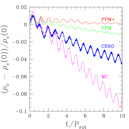
Figure 2: Normalized error in the central rest-mass density for star A with different reconstruction methods. All runs are axisymmetric and equatorially symmetric with a resolution of $64^{2}$ and outer boundaries at $7.1M$. With PPM, the drift in the central density is strongly reduced with respect to the MC and CENO results. With PPM⁺, the central density drift disappears almost entirely.

Next we check the ability of our code to distinguish radially stable from radially unstable stars. We consider two uniformly rotating stars, stars A and B, which are members of a constant angular momentum sequence, $J=0.01$ in our $G=c=\kappa=1$ units. The $J=0.01$ sequence has a turning-point at central rest-mass density $\rho_{c}^{\rm crit}=0.31$, which has the maximum mass $M_{\rm max}=0.172$ for the sequence. For a sequence of uniformly rotating stars, this turning point marks the onset of secular, not dynamical, radial instability fis88 , but prior numerical simulations dmsb03 have found the point of onset of dynamical instability to be very close to the point of onset of secular instability. We pick two similar stars on either side of the onset of secular instability: star A with initial central rest-mass density $\rho_{c}(0)=0.24$ on the stable branch and Star B with $\rho_{c}(0)=0.37$ on the unstable branch. In Fig. 3, we see that the code correctly finds star A to be stable and star B to be unstable.

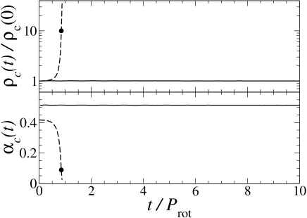
Figure 3: Axisymmetric evolution of uniformly rotating stars. Star A (solid lines) is stable, while star B (dashed lines) is unstable to collapse. The upper window shows the central density normalized to its initial value, while the lower gives the central lapse. The solid dot indicates the first appearance of an apparent horizon during the collapse of star B.

Figure 4: Snapshots of the rest density contours and the velocity field $(v^{x},v^{z})$ in the meridional plane during the axisymmetric collapse of uniformly rotating star B to a Kerr black hole. The contour lines are drawn for $\rho_{0}=10^{-(0.3j+0.09)}\rho_{0}^{Max}$ for $j=0,1,..,12$, where $\rho_{0}^{Max}$ is the maximum of $\rho_{0}$ at the time of excision. The thick dashed curve marks the excision zone. The thick solid curve is the apparent horizon. We show the system at the time of excison (upper panel), at the time at which the last of the matter falls into the excision region (middle panel), and at a late time just prior to the termination of the integration (lower panel).

Star B collapses to a black hole. Without excision, the extreme density and spacetime curvature at the center of the collapsing star cause the code to crash shortly after the formation of an apparent horizon which envelops some, but not all, of the star. The evolution can be continued by excising a region inside the horizon. When we do this, we find that all of the matter falls into the hole within a few $M$ of the time excision is introduced, leaving a vacuum Kerr black hole with roughly the same $M$ and $J$ as the initial star B. We then continue to evolve for another $30M$. We find that the hole’s angular momentum, computed as the sum of surface and volume integrals, decreases with time, and this angular momentum drift limits the length of time that our evolution remains accurate. Comparable angular momentum loss was also present in dsy04 . Since this drift appears after most of the matter has fallen into the excision region, the source of the error resides in the evolution of the BSSN variables. Since we use the same algorithm to evolve the metric as in dsy04 , it is not surprising that the $J$-drift has the same magnitude. We simulated the collapse of star B on both $64^{2}$ and $128^{2}$ grids, and we found, as in dsy04 , that the $J$-drift converges to zero with increasing resolution. In Fig. 4, we show snapshots from our post-excision evolution on the $128^{2}$ grid footnote:ex . To check that the final geometry corresponds to a stationary Kerr spacetime, we confirm that the area and the equatorial and polar circumferences of the apparent horizon agree with the appropriate values for a Kerr black hole with the $M$ and $J$ of our spacetime to better than 1% (see dsy04 for details).

We now demonstrate the ability of our code to handle differential rotation in both 2D and 3D by considering the evolution of star C, a stable, hypermassive, differentially rotating star. We evolved this star in axisymmetry with PPM⁺ using a fairly low resolution of $48^{2}$ zones and outer boundaries at $7.1M$. Figure 5 shows the angular velocity profile at several times during this evolution, and demonstrates that our code correctly maintains the differential rotation. Slight errors in the angular velocity arise near the origin. The central angular velocity is particularly susceptible to error, as its calculation involves dividing the local azimuthal velocity by the (small) radius. During the first $15P_{\rm rot}$ of this evolution (where $P_{\rm rot}$ refers to the central rotation period), the central density remains within $5\%$ of its initial value and the ADM mass is conserved to within $0.5\%$, even at this low resolution. (The angular momentum computed as a volume integral over all space is conserved exactly in our code in axisymmetry.) During this period, the normalized Hamiltonian and momentum constraints (see dmsb03 for definition) are $\sim 1~{}\%$.

Figure 5: Snapshots of the angular velocity profile for an evolution of the differentially rotating star C in axisymmetry ($48^{2}$) with outer boundaries at $7.1M$. The profile is well-maintained in the bulk of the star for over 15 central rotation periods ($P_{\rm rot}$).

Next, we compare the axisymmetric run of star C described above with an equivalent 3D run in equatorial symmetry. The 3D run was performed with a $96^{2}\times 48$ grid in $(x,y,z)$ and outer boundaries at $7.1M$, so that the grid cell size is the same as in the 2D run. The deviations in the central density for these two runs are compared in Fig. 6, which shows that the axisymmetric and full 3D runs have comparable errors. For $t\lesssim 6P_{\rm rot}$, the two runs are similar and the angular velocity profiles agree very well. After this time, however, the star in the 3D run begins to move away from the center of the grid, eventually making contact with the outer grid boundary. This is due to accumulated error in the linear momentum and is a well known problem associated with evolutions of stars in equatorial symmetry nct00 . In our simulations, the effect can be reduced by improving spatial resolution. By comparing runs of star C on $64^{2}\times 32$, $96^{2}\times 48$, and $168^{2}\times 84$ grids, we find that the movement of the center of mass converges to zero at third-order in spatial resolution. We note that the drift can be removed at any resolution by employing $\pi$-symmetry, so that the symmetry boundary conditions tie the star to the center of the grid.

Figure 6: Fractional error in the central density versus time for evolutions of star C in 2D and 3D. The 3D run was performed in equatorial symmetry with resolution $96^{2}\times 48$ with outer boundaries at $7.1M$. The axisymmetric run has the same spatial resolution (grid cell size) as the 3D case, and thus employs a $48^{2}$ grid with boundaries at $7.1M$. The errors in the central density are of the same order for both runs.

IV.2 Minkowski Spacetime MHD Tests

Komissarov k99 has proposed a suite of challenging one-dimensional tests of nonlinear, relativistic MHD waves in Minkowski spacetime. Most of the tests (except the nonlinear Alfvén wave test) start with discontinuous initial data at $x=0$ (see Table 2), with homogeneous profiles on either side. We integrate the MHD equations from $t=0$ to $t=t_{\rm final}$, where $t_{\rm final}$ is specified in Table 2 for each case. The gas satisfies a $\Gamma$-law EOS with $\Gamma=4/3$. In all the cases, our computational domain is $x\in(-2,2)$. Our standard resolution is $\Delta x=0.01$ (400 grid points). We are able to integrate all the cases using the MC resconstruction scheme and with a Courant factor of 0.5. Thus, the number of timesteps for a given test is $t_{\rm final}/(0.5\Delta x)=200t_{\rm final}$. With PPM resconstruction scheme, we need to lower the Courant factor to 0.4 for the fast shock test. We obtain slightly better results with PPM resconstruction scheme for the shock tube tests 1 and 2. The two resconstruction schemes give comparable results for the other tests. Here we present the simulations using the MC resconstruction scheme. Figures 7–9 compare our simulation results (symbols) with the expected results (solid lines) ko_exact . Our numerical results are similar to those reported recently for other codes k99 ; HARM . Below, we briefly discuss each of the cases we studied.

Table 2: Initial states for one-dimensional MHD tests.^a

Test	Left state	Right State	$t_{\rm final}$
Fast Shock	$u^{i}=(25.0,0.0,0.0)$	$u^{i}=(1.091,0.3923,0.00)$	2.5
($\mu=0.2{}^{\rm b}$)	$B^{i}/\sqrt{4\pi}=(20.0,25.02,0.0)$	$B^{i}/\sqrt{4\pi}=(20.0,49.0,0.0)$
	$P=1.0$, $\rho_{0}=1.0$	$P=367.5$, $\rho_{0}=25.48$
Slow Shock	$u^{i}=(1.53,0.0,0.0)$	$u^{i}=(0.9571,-0.6822,0.00)$	2.0
($\mu=0.5{}^{\rm b}$)	$B^{i}/\sqrt{4\pi}=(10.0,18.28,0.0)$	$B^{i}/\sqrt{4\pi}=(10.0,14.49,0.0)$
	$P=10.0$, $\rho_{0}=1.0$	$P=55.36$, $\rho_{0}=3.323$
Switch-off Fast	$u^{i}=(-2.0,0.0,0.0)$	$u^{i}=(-0.212,-0.590,0.0)$	1.0
Rarefaction	$B^{i}/\sqrt{4\pi}=(2.0,0.0,0.0)$	$B^{i}/\sqrt{4\pi}=(2.0,4.71,0.0)$
	$P=1.0$, $\rho_{0}=0.1$	$P=10.0$, $\rho_{0}=0.562$
Switch-on Slow	$u^{i}=(-0.765,-1.386,0.0)$	$u^{i}=(0.0,0.0,0.0)$	2.0
Rarefaction	$B^{i}/\sqrt{4\pi}=(1.0,1.022,0.0)$	$B^{i}/\sqrt{4\pi}=(1.0,0.0,0.0)$
	$P=0.1$, $\rho_{0}=1.78\times 10^{-3}$	$P=1.0$, $\rho_{0}=0.01$
Shock Tube 1	$u^{i}=(0.0,0.0,0.0)$	$u^{i}=(0.0,0.0,0.0)$	1.0
	$B^{i}/\sqrt{4\pi}=(1.0,0.0,0.0)$	$B^{i}/\sqrt{4\pi}=(1.0,0.0,0.0)$
	$P=1000.0$, $\rho_{0}=1.0$	$P=1.0$, $\rho_{0}=0.1$
Shock Tube 2	$u^{i}=(0.0,0.0,0.0)$	$u^{i}=(0.0,0.0,0.0)$	1.0
	$B^{i}/\sqrt{4\pi}=(0.0,20.0,0.0)$	$B^{i}/\sqrt{4\pi}=(0.0,0.0,0.0)$
	$P=30.0$, $\rho_{0}=1.0$	$P=1.0$, $\rho_{0}=0.1$
Collision	$u^{i}=(5.0,0.0,0.0)$	$u^{i}=(-5.0,0.0,0.0)$	1.22
	$B^{i}/\sqrt{4\pi}=(10.0,10.0,0.0)$	$B^{i}/\sqrt{4\pi}=(10.0,-10.0,0.0)$
	$P=1.0$, $\rho_{0}=1.0$	$P=1.0$, $\rho_{0}=1.0$
Nonlinear Alfvén wavec	$u^{i}=(0.0,0.0,0.0)$	$u^{i}=(3.70,5.76,0.00)$	2.0
($\mu=0.626{}^{\rm b}$)	$B^{i}/\sqrt{4\pi}=(3.0,3.0,0.0)$	$B^{i}/\sqrt{4\pi}=(3.0,-6.857,0.0)$
	$P=1.0$, $\rho_{0}=1.0$	$P=1.0$, $\rho_{0}=1.0$

^a In all cases, the gas satisfies the $\Gamma$-law EOS with $\Gamma=4/3$. For the first 7 tests, the left state refers to $x<0$ and the right state, $x>0$.

^b $\mu$ is the speed at which the wave travels

^c For the nonlinear Alfvén wave, the left and right states are joined by a continuous function. See k97 or Appendix B for details.

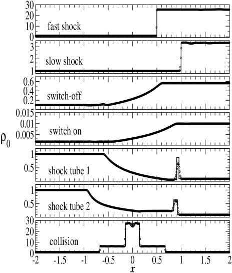
Figure 7: Density profiles for the nonlinear wave tests at $t=t_{\rm final}$ (see Table 2). Symbols denote data from numerical simulations with resolution $\Delta x=0.01$. Solid lines in the upper 6 panels denote the exact solutions ko_exact . The solid line in the last panel denotes a numerical simulation with higher resolution, $\Delta x=10^{-3}$.

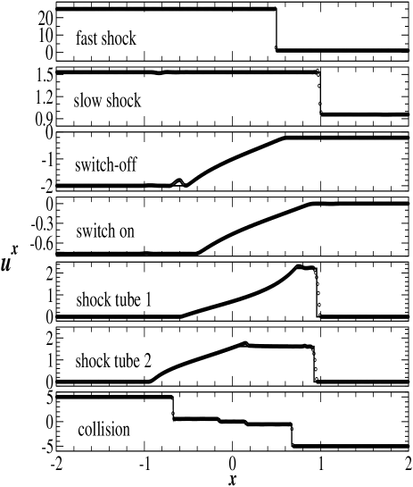
Figure 8: Velocity profiles ($u^{x}$) for the nonlinear wave tests at $t=t_{\rm final}$. Symbols denote data from numerical simulations with resolution $\Delta x=0.01$. Solid lines in the upper 6 panels denote the exact solutions ko_exact . The solid line in the last panel denotes a numerical simulation with higher resolution, $\Delta x=10^{-3}$.

Fast and slow shocks In these tests, the initial MHD variables on the left ($x<0$) and right ($x>0$) satisfy the special relativistic Rankine-Hugoniot jump conditions for MHD shocks ma87 . As a result, the discontinuity simply travels with a certain speed $\mu$ without changing its pattern. The fast shock is the most relativistic case of all the tests. In the shock frame, the Lorentz factor of the upstream flow is $u^{0}\approx 25$. The shock moves with a speed $\mu=0.2$. The slow shock is not as strong and it moves with a faster speed ($\mu=0.5$). Our simulations for these two tests agree quite well with the exact solutions. In the slow shock test, we see small oscillations (due to numerical artifacts) in density on the right side of the shock (see Fig. 7). This numerical artifact is also seen in simulations with other codes k99 ; HARM . We have performed simulations on these two cases using different resolutions and found that the errors converge to first order in $\Delta x$, which is expected for problems with discontinuities in the computational domain.

Switch-on/off rarefaction In these tests, the left and right states are connected by a rarefaction wave at $t>0$. The tests become more challenging when the tangential component of the magnetic field (i.e., $B^{y}$) is switched on/off when going from the right state to the left state. The exact solutions are obtained by integrating a system of ordinary differential equations (see e.g., k99 ; c70 ). Our simulation results agree with the exact solutions very well, except that we see numerical artifacts near the trailing edge of the rarefaction wave in the switch-off test. We also observe a small oscillation (not visible on the scale shown in Figs. 7 and 8) near the leading edge of the rarefaction wave in the switch-on test. These numerical artifacts are also seen in simulations with other codes k99 ; HARM . As explained in k99 , the oscillation results from perturbations created by numerical dissipation during the initial stage when the wavefront is very steep. The perturbations propagate across the main wave and then separate from it.

Shock tubes 1 and 2 The initial left and right states are given in Table 2. At time $t>0$, the left and right states are connected by a rarefaction wave, a contact discontinuity and a shock wave. The exact solution can be computed using a method similar to t86 . In the shock tube 1 test, the solution consists of a thin layer of shocked gas, which is poorly resolved in our simulation and has a wrong value of shell density. The thin layer is covered by only 5 grid points with our resolution. We found that the correct density is obtained in higher resolution simulations in which $\Delta x\lesssim 0.0035$, which provides $\gtrsim$ 12 grid points across the thin layer. Our results in these two tests are comparable to those reported in k99 ; HARM .

Collision In this test, the flows on both sides travel with equal speed but in opposite directions. The tangential component of the magnetic field is also equal in magnitude but opposite in direction. We do not have the exact solution for this test. Thus, we compare our lower-resolution ($\Delta x=0.01$) simulation with a high-resolution one ($\Delta x=10^{-3}$). The lower-resolution simulation results are qualitatively the same as the results reported in HARM , but not as good as the results of Komissarov k99 , who uses a more sophisticated Riemann solver.

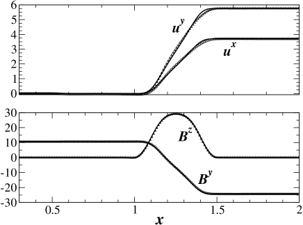
Figure 9: Nonlinear Alfvén wave test. Symbols are simulation results with resolution $\Delta x=0.01$ and solid lines are the exact solution. The profiles are shown at time $t=t_{\rm final}=2.0$. Our computational domain is $x\in(-2,2)$. We only show the region $0.3\leq x\leq 2.0$ in this graph.

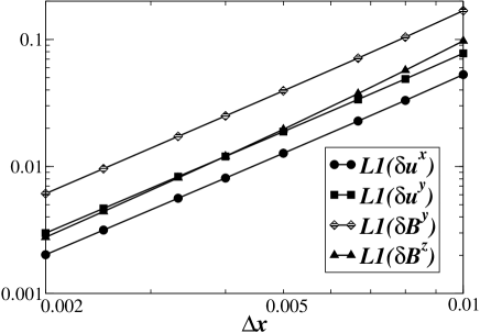
Figure 10: L1 norms of the errors in $u^{x}$, $u^{y}$, $B^{y}$ and $B^{z}$ for the nonlinear Alfvén wave test at $t=t_{\rm final}=2.0$. This log-log plot shows that the L1 norms of the errors in $u^{x}$, $u^{y}$ and $B^{y}$ are proportional to $(\Delta x)^{2}$, and are thus second-order convergent. The error in $B^{z}$ goes as a slightly higher power of $\Delta x$.

Nonlinear Alfvén Wave The initial data for this test are qualitatively different from the other seven tests. The left ($x<-W/2$) and right ($x>W/2)$ states are separated by a width $W=0.5$ at $t=0$. The two states are joined by continuous functions in the region $x\in(-W/2,W/2)$ at $t=0$. The details of the setup of initial data can be found in k97 , which we summarize in Appendix B. The pattern should simply move with a constant speed $\mu=0.626$. Figure 9 shows the simulation results (symbols) and exact solution (solid lines). The simulation results are again similar to k99 . Since there are no discontinuities in this problem, we expect the errors to converge at second order in $\Delta x$. To demonstrate this, we consider a grid function $g$ with error $\delta g=g-g^{\rm exact}$. We calculate the L1 norm of $\delta g$ (the “average” of $\delta g$) by summing over every grid point $i$:

$$L1(\delta g)\equiv\Delta x\sum_{i=1}^{N}|g_{i}-g^{\rm exact}(x_{i})|\ ,$$ (69)

where $N\propto 1/\Delta x$ is the number of grid points. Figure 10 shows the L1 norms of the errors in $u^{x}$, $u^{y}$, $B^{y}$ and $B^{z}$ at $t=t_{\rm final}=2.0$. We find that the errors in $u^{x}$, $u^{y}$ and $B^{y}$ converge at second order in $\Delta x$. The error in $B^{z}$ converges at slightly better than second order in $\Delta x$.

IV.3 Curved Background Tests:
  Relativistic Bondi Flow

Next, we test the ability of our code to accurately evolve the relativistic MHD equations in the strong gravitational field near a black hole. Specifically, we check its ability to maintain stationary, adiabatic, spherically symmetric accretion onto a Schwarzschild black hole, in accord with the relativistic Bondi accretion solution st83 . It has been shown that the relativistic Bondi solution is unchanged in the presence of a divergenceless radial magnetic field dVh03 . The advantages of this test are that it involves strong gravitational fields and relativistic flows, and that there exists an analytic solution with which to test our results. We write the metric in Kerr-Schild (ingoing Eddington-Finklestein) coordinates; in this way, all the variables are well behaved at the horizon (“horizon penetrating”), and the excision radius can be placed inside the event horizon. We begin by holding the metric field variables fixed in order to prevent the black hole from growing due to accretion. With the metric fixed, the flow is exactly stationary in the continuous limit. When evolved with a finite-difference code, discretization errors will cause small deviations in the flow from its initial state. These deviations should converge to zero as resolution is increased. Eventually, the system may settle down to an equilibrium solution of the descretized hydrodynamic equations. To diagnose the behavior of our code, we introduce two variables. The deviation of the fluid configuration from the analytic Bondi solution we measure by $\delta\rho_{\star}$, the L1 norm in 3D of $\left|\rho_{\star}-\rho_{\star}^{\rm exact}\right|$ (where $\rho_{\star}^{\rm exact}$ is the analytic value of $\rho_{\star}$), normalized by the rest mass:

$$\delta\rho_{\star}\equiv\frac{\Delta x\Delta y\Delta z\sum_{i,j,k}|\rho_{\star i,j,k}-\rho_{\star}^{\rm exact}(x_{i},y_{j},z_{k})|}{\Delta x\Delta y\Delta z\sum_{i,j,k}\rho_{\star}^{\rm exact}(x_{i},y_{j},z_{k})}\ .$$ (70)

To measure the settling down of the solution to a numerical equilibrium, we monitor $\Delta\rho_{b}$, the L2 norm of $\dot{\rho}_{b}\Delta t$:

$$\Delta\rho_{b}\equiv\Delta t\Delta x\Delta y\Delta z\left[\sum_{i,j,k}(\dot{\rho}_{b})_{i,j,k}^{2}\right]^{1/2}\ .$$ (71)

The quantities $\delta\rho_{\star}$ and $\Delta\rho_{b}$ were chosen because they correspond to the diagnosics used to monitor Bondi accretion test problems in HARM and dsy04 , respectively.

Figure 11: Unmagnetized Bondi accretion onto a Schwarzschild black hole. Four different methods are compared: MC reconstruction, CENO reconstruction, and PPM reconstruction, both with and without Kreiss-Oliger (KO) dissipation. Each run was performed on a $64^{2}$ grid using axisymmetry.

For this test, we evolve the same configuration used by hsw84 , dVh03 , and HARM . The sonic radius is at Schwarzschild (areal) radius $r_{s}=8M$, the accretion rate is $\dot{M}=1$, and the equation of state is $\Gamma=4/3$. As in HARM , we set our excision radius at $r_{\rm ex}=1.9M$ (the horizon is at $2M$) and evolve for $100M$. (We find that the system settles to equilibrium long before $100M$.) We place outer boundaries at $10M$, at which point the analytic values of the conserved variables are imposed.

First, we evolve this accretion flow in the absence of a magnetic field. In Figure 11, we show the results for an axisymmetric grid of $64^{2}$ using various numerical techniques. We find that using MC reconstruction gives much better results than using PPM. This is probably due to the larger numerical diffusivity in the MC scheme which stabilizes spurious numerical oscillations. PPM can be “corrected,” however, by adding a small dissipation. In hln05 , the oscillations are removed by shifting the numerical spatial stencil in supersonic flow. We have instead addressed the problem by adding a small Kreiss-Oliger dissipation ko73 . We find that PPM with Kreiss-Oliger dissipation performs as well as MC for this problem (see Fig. 11). We have also evolved an accretion flow with small $\dot{M}$ while allowing the metric to evolve. We find that the flow is stable, and that, as expected, the irreducible mass of the black hole slowly increases fn:bondi . The MHD variables remain near the Bondi equilibrium initial values until the black hole grows appreciably.

Figure 12: $\delta\rho_{\star}$ after $100M$ for various initial values of $b^{2}/\rho_{0}|_{r=2M}$. PPM with Kreiss-Oliger dissipation is used in each run. Results from $64^{2}$ and $128^{2}$ grid runs are compared. The $\delta\rho_{\star}$ found with the $128^{2}$ grid is multiplied by 4 to allow scaling to be checked for second order convergence.

Next, we evolve with a radial magnetic field. In the continuum limit, the magnetic forces cancel exactly. However, the cancellation will not be exact in a finite-difference code, and this test can be quite difficult for a GRMHD code when the magnetic field is strong.

In Fig. 12, we plot the error, measured by $\delta\rho_{\star}$ after $100M$ of evolution, for 2D (axisymmetric) runs with various values of $b^{2}/\rho_{0}$ at the horizon. We use the PPM reconstruction method with Kreiss-Oliger dissipation for each run. In order to test convergence, we use both $64^{2}$ and $128^{2}$ grids. We are able to evolve with magnetic fields $b^{2}/\rho_{0}|_{r=2M}\lesssim 30$. Stronger radial fields quickly crash the code. For $b^{2}/\rho_{0}|_{r=2M}\lesssim 5$, we find that $\delta\rho_{\star}$ settles quickly to a final value. For larger $b^{2}/\rho_{0}|_{r=2M}$, $\delta\rho_{\star}$ does not settle as well, but the results are still second-order convergent after $100M$. Evolving with MC gives better “settling” behavior for $5\lesssim b^{2}/\rho_{0}|_{r=2M}\lesssim 30$, but it is still not possible to evolve flows with $b^{2}/\rho_{0}|_{r=2M}\gtrsim 30$. Gammie, McKinney, and Tóth HARM are able to evolve with much higher $b^{2}/\rho_{0}|_{r=2M}$. This is probably due to their use of a spherical-polar coordinate grid, which is better adapted to the spherical symmetry of this problem than our cylindrical grid.

We have also evolved the Bondi flow in three dimensions on $64^{3}$ grids using octant symmetry. We find that we can maintain equilibrium flow for $b^{2}/\rho_{0}|_{r=2M}\lesssim 10$ in 3D.

IV.4 Dynamical Background Tests: Gravitational Wave-Induced MHD Waves

To test the capability of our code to handle dynamical gravitational and MHD fields simultaneously, we consider a gravitational wave oscillating in an initially homogeneous, uniformly magnetized fluid. The gravitational wave will, in general, induce Alfvén and magnetosonic waves moortgat03 ; moortgat04 ; kallberg04 . In a companion paper dlss05b (hereafter, Paper II), we perform a detailed analysis of this problem and provide an analytic solution for the perturbations in a form which is suitable for comparison with numerical results.

This test problem is one-dimensional. We consider a linear, standing gravitational wave whose amplitude varies in the $z$-direction:

$$h_{+}(t,z) = h_{+0}\sin\!kz\cos\!kt\ ,$$ (72)

$$h_{\times}(t,z) = h_{\times 0}\sin\!kz\cos\!kt\ ,$$ (73)

where $k$ is the wave number, and $h_{+0}$ and $h_{\times 0}$ are constants. We assume that at $t=0$, the magnetized fluid is unperturbed:

$$P(0,z)=P_{0}\ ,\ \ \ \ \ \ \ \ \ \ \rho_{0}(0,z)=\rho_{0}\ ,$$ (74)

$$v^{i}(0,z)=0\ ,\ \ \ \ \ \ \ \ \ \ B^{i}(0,z)=B_{0}^{i}\ .$$ (75)

Subsequently, the gravitational wave excites the MHD modes of the fluid. As discussed in Paper II, the gravitational wave is unaffected by the fluid to linear order, and the metric perturbation, $h_{\mu\nu}(t,z)$, in the transverse-traceless (TT) gauge can be calculated from Eqs. (72) and (73). The perturbations in pressure $\delta P(t,z)$, velocity $\delta v^{i}(t,z)$, and magnetic field $\delta B^{i}(t,z)$ can be computed analytically as shown in Paper II. Our analytic solutions are valid as long as we are in the linear regime in which the following three inequalities hold (see Paper II):

$$|h^{\mu\nu}|\sim h_{0} \ll 1\ ,$$ (76)

$$\frac{|T^{\mu\nu}|}{|h^{\mu\nu}|}\sim\frac{\cal E}{h_{0}} \ll k^{2}\ ,$$ (77)

$$t\ll 1/\sqrt{|T_{\mu\nu}|} \sim 1/\sqrt{\cal E},$$ (78)

where $h_{0}=\sqrt{h_{+0}^{2}+h_{\times 0}^{2}}$ and ${\cal E}=\rho_{0}(1+\epsilon_{0})+P_{0}+b_{0}^{2}$.

The analytic solution is a superposition of the three eigenmodes of the homogeneous system (the Alfvén, slow magnetosonic, and fast magnetosonic waves) and a particular solution which oscillates at the frequency of the gravitational wave. The induced Alfvén wave obeys the dispersion relation

$$\omega^{2}=\omega_{A}^{2}\equiv(\mbox{\boldmath$k$}\cdot\mbox{\boldmath$v$}_{A})^{2}\ ,$$ (79)

where $\mbox{\boldmath$k$}=k\hat{\mbox{\boldmath$z$}}$ is the wave vector associated with the standing gravitational wave, and $\mbox{\boldmath$v$}_{A}=\mbox{\boldmath$B$}_{0}/\sqrt{4\pi{\cal E}}$ is the Alfvén velocity. This mode gives rise to a velocity perturbation

$$\delta{\mbox{\boldmath$v$}}\propto\tilde{\mbox{\boldmath$u$}}_{A}\equiv\mbox{\boldmath$k$}\times\mbox{\boldmath$v$}_{A}.$$ (80)

The frequencies of the induced slow and fast magnetosonic modes, $\omega_{m1}$ and $\omega_{m2}$, are found by solving the following dispersion relation for $\omega^{2}$:

$$\omega^{4}-[k^{2}c_{m}^{2}+c_{s}^{2}(\mbox{\boldmath$k$}\cdot\mbox{\boldmath$v$}_{A})^{2}]\omega^{2}+k^{2}c_{s}^{2}(\mbox{\boldmath$k$}\cdot\mbox{\boldmath$v$}_{A})^{2}=0\ ,$$ (81)

where $c_{m}^{2}=v_{A}^{2}+c_{s}^{2}(1-v_{A}^{2})$. For the corresponding eigenvectors, one has:

$$\delta\mbox{\boldmath$v$}\propto\tilde{\mbox{\boldmath$u$}}_{mi}\equiv\mbox{\boldmath$v$}_{A}+\frac{\omega_{mi}^{2}(1-v_{A}^{2})}{(\omega_{mi}^{2}-k^{2})(\mbox{\boldmath$k$}\cdot\mbox{\boldmath$v$}_{A})}\mbox{\boldmath$k$}\ \ i=1,2\ .$$ (82)

Note that $\tilde{\mbox{\boldmath$u$}}_{A}$ is orthogonal to $\tilde{\mbox{\boldmath$u$}}_{m1}$ and $\tilde{\mbox{\boldmath$u$}}_{m2}$, but $\tilde{\mbox{\boldmath$u$}}_{m1}$ and $\tilde{\mbox{\boldmath$u$}}_{m2}$ are not, in general, orthogonal to each other.

The setup for our code test is as follows. Our computational domain is $z\in(-1,1)$. We choose $k=2\pi$ so that our computational domain covers two wavelengths of the gravitational wave. Our standard resolution is $\Delta z=0.01$ (200 grid points). At time $t=0$, we assign the metric $g_{\mu\nu}(0,z)=\eta_{\mu\nu}+h_{\mu\nu}(0,z)$, where $\eta_{\mu\nu}=\rm{diag}(-1,1,1,1)$ is the Minkowski metric, and the nonzero components of $h_{\mu\nu}(0,z)$ are:

$$h_{xx}(0,z) = -h_{yy}(0,z)=h_{+}(0,z)\ ,$$ (83)

$$h_{xy}(0,z) = h_{yx}(0,z)=h_{\times}(0,z)\ .$$ (84)

We choose geodesic slicing and zero shift ($\alpha=1$, $\beta^{i}=0$) as our gauge conditions. Hence we set the initial extrinsic curvature to zero ($K_{ij}(0,z)=0$) in accord with our gauge choices and Eqs. (72), (73), and (2). We also set the MHD variables at $t=0$ according to Eqs. (74) and (75). We choose the adiabatic index $\Gamma=4/3$ in all of our simulations in this section. Periodic boundary conditions on both matter and gravitational field quantities are enforced at the upper and lower boundaries in $z$. We expect that the metric, as well as the MHD quantities, in our full GRMHD simulations should agree with the analytic solutions given in Paper II to linear order as long as the inequalities in Eqs. (76)–(78) are satisfied.

IV.4.1 A General Example

We first consider a general case in which all three of the MHD modes are excited. We take the following initial data:

$$\rho_{0}=2.78\times 10^{-9}\ ,\ \ \ P_{0}=1.29\times 10^{-9}\ ,$$

$$B_{0}^{i}=(1.09,8.26,14.4)\times 10^{-5}\ ,$$

$$h_{+0}=h_{\times 0}=1.18\times 10^{-4}\ .$$ (85)

Figure 13 gives a comparison of the analytic and numerical solutions for three selected perturbed variables. The perturbations are plotted with respect to time for a chosen location on the grid ($z=1/8$). Good agreement is shown between the numerical and analytic values for many periods of the gravitational wave. We also find very good agreement for the metric quantities $g_{xx}$ and $g_{xy}$ in our simulation and the analytic values calculated from Eqs. (72) and (73). The pressure perturbation, however, differs from the analytic solution by a slight secular drift. (In fact, all variables eventually exhibit a drift away from the analytic solution, but the drift is first noticeable in the case of the pressure.)

Figure 13: Analytic and numerical solutions for the perturbations of a magnetized fluid due to the presence of a gravitational wave (see Section IV.4.1). The thick solid and thin dotted lines represent, respectively, the analytic and numerical solutions, though the two lines are not readily distinguishable in plots (a) and (b). All quantities are evaluated at $z=1/8$ and are normalized as indicated. Time is normalized by the gravitational wave period.

Figure 14: Relative error in the pressure perturbation (evaluated at $z=1/8$) for three different initial data sets. The solid lines give the numerical results while the dashed lines give the fits from Eq. (86). The three initial data sets are derived from the standard case in Eq. (85) by taking $\{\rho_{0},\,P_{0}\}^{\rm new}=\xi\{\rho_{0},\,P_{0}\}^{\rm old}$, $(B^{i}_{0})^{\rm new}=\sqrt{\xi}(B^{i}_{0})^{\rm old}$, and $\{h_{+0},\,h_{\times 0}\}^{\rm new}=\zeta\{h_{+0},\,h_{\times 0}\}^{\rm old}$, where $\xi$ and $\zeta$ are constants and “old” refers to the values in Eq. (85). (Effectively, $T_{\mu\nu}^{\rm new}=\xi T_{\mu\nu}^{\rm old}$ and $h_{0}^{\rm new}=\zeta h_{0}^{\rm old}$.) The regime of validity for the analytic solution is approached for small $h_{0}$ and $|T_{\mu\nu}|/h_{0}$ (see Eqs. (76) and (77)), or equivalently, for decreasing $\zeta$ and $\xi/\zeta$. For the curves shown, these values are: (a) $\zeta=3$, $\xi/\zeta=3$, (b) $\zeta=2$, $\xi/\zeta=2$, and (c) $\zeta=1$, $\xi/\zeta=1$. Moving from (a) to (c), we find that the relative error decreases as expected and that the errors are well fit by Eq. (86). Note that the normalization differs in the three cases to reflect the differing values of $P_{0}$ and $h_{0}$.

Figure 15: Velocity projected along the direction of the Alfvén mode eigenvector ($\delta v_{A}\equiv\delta\mbox{\boldmath$v$}\cdot\tilde{\mbox{\boldmath$u$}}_{A}/|\tilde{\mbox{\boldmath$u$}}_{A}|$), for the case discussed in Section IV.4.1 (the general case). (a) Analytic and numerical plots of the projected velocity. (The curves cannot be distinguished on this scale.) (b) Contributions to the analytic solution for $\delta v_{A}/h_{0}$. The particular solution (dashed) and Alfvén wave (dotted) contributions added together give the total perturbation (solid line). All quantities are evaluated at $z=1/8$.

Figure 16: Velocity projected along the direction of the slow magnetosonic mode eigenvector ($\delta v_{m2}\equiv\delta\mbox{\boldmath$v$}\cdot\tilde{\mbox{\boldmath$u$}}_{m2}/|\tilde{\mbox{\boldmath$u$}}_{m2}|$), for the same case as in Figure 15. (a) Analytic and numerical plots of the projected velocity. (b) Contributions to the analytic solution for $\delta v_{m2}/h_{0}$. The fast magnetosonic (dotted), slow magnetosonic (short dashed), and particular solution (long dashed) contributions added together give the total perturbation (solid line). All quantities are evaluated at $z=1/8$.

This secular drift is not due to numerical error, but rather is an effect of the nonlinear terms which are neglected in our analytic solution. To show that it is not a numerical error, we performed simulations at resolutions of 50, 100, and 200 grid points, and we found convergence to second order to a solution with nonzero drift. Since the discrepancy is due to nonlinear terms, choosing smaller (larger) initial mass-energy density and smaller (larger) gravitational wave strength leads to a smaller (larger) discrepancy with the analytic solution. In particular, the size of the discrepancy is controlled by the degree to which the conditions in Eqs. (76)–(78) are satisfied. By evolving a range of initial data sets in which we independently varied $h_{0}$ and ${\cal E}/h_{0}$, as well as initial data sets with $h_{0}=0$ (no gravity wave), we found that the numerical solution for the pressure perturbation ($\delta P$) is always well fit by the relation

$$\delta P=\left\{\begin{array}[]{ll}\delta P_{\rm ana}+h_{0}P_{0}(c_{1}h_{0}+c_{2}{\cal E}/h_{0})t^{2}&(h_{0}\neq 0)\\ c_{2}P_{0}{\cal E}t^{2}&(h_{0}=0)\ ,\end{array}\right.$$ (86)

where $t$ is the coordinate time, $\delta P_{\rm ana}$ is the analytic solution for the pressure perturbation given in Paper II, and $c_{1}$ and $c_{2}$ are constants (see Fig. 14). (Note that the coefficient $h_{0}P_{0}$ is simply the typical scale of the pressure perturbation.) The term proportional to $c_{1}$ corresponds to nonlinear effects of the gravitational wave on the fluid, while the term proportional to $c_{2}$ is related to the self-gravity of the fluid footnote:hcon . Neither of these effects are accounted for in our analytic solution [see Eqs. (76)–(78)]. Thus, the disagreement of the numerical and analytic results may be reduced by choosing initial data with smaller $h_{0}$ and ${\cal E}/h_{0}$.

To extract the various MHD modes in this test, we have performed two projections of the velocity. Figure 15a shows the numerical and analytic values of the projection along $\tilde{\mbox{\boldmath$u$}}_{A}$ (again evaluated at $z=1/8$). Because we have projected the velocity along the direction of the Alfvén mode eigenvector, which is orthogonal to the fast and slow mode eigenvectors, we only pick up contributions from the Alfvén wave and the particular solution (see Paper II for the analytic expression of the particular solution). The lower panel shows these individual contributions along with the total. One can see that both the Alfvén and particular components contribute significantly to the velocity perturbation in this direction. Next, Fig. 16 shows the projection of the velocity along the direction of the slow mode eigenvector. This time, there are contributions from the slow and fast modes in addition to the particular solution, and one again sees that all modes are contributing strongly. (The slow and fast modes are both present in this velocity projection since $\tilde{\mbox{\boldmath$u$}}_{m1}$ and $\tilde{\mbox{\boldmath$u$}}_{m2}$ are not orthogonal.) Figures 15 and 16, taken together, show that our code correctly manifests all three MHD waves, in addition to the particular solution contribution.

Table 3: Evaluation of Methods

Method	Characterization
	Equilibrium Stars	Shocks	Alfvén Waves
HLL+PPM/HLL+CT	performs well	performs well	performs well
HLL+CENO/HLL+CT	central density drifts	performs well	performs well
HLL+MC/HLL+CT	central density drifts	performs well	performs well
HLL+MC/VP	central density drifts	unacceptable oscillations	acceptable
non-conservative/CT	performs well	problems for high $b^{2}/\rho_{0}$	problems for high $b^{2}/\rho_{0}$

IV.4.2 Special Cases

To further test our code, we consider several initial data sets with special properties. Starting with the initial data set given in Eq. (85), we hold ${\cal E}$ and $h_{0}$ constant but change the balance between the plus and cross modes so that the magnetosonic modes are not excited. As explained in Paper II [in particular, see Eq. (93) and surrounding discussion], this occurs when $h_{+0}$ and $h_{\times 0}$ satisfy the equation

$$[(B_{0}^{y})^{2}-(B_{0}^{x})^{2}]h_{+0}-2B_{0}^{x}B_{0}^{y}h_{\times 0}=0\ .$$ (87)

Thus, we obtain the new initial data set:

$$\rho_{0}=2.78\times 10^{-9}\ ,\ \ \ P_{0}=1.29\times 10^{-9}\ ,$$

$$B_{0}^{i}=(1.09,8.26,14.4)\times 10^{-5}\ ,$$

$$h_{+0}=4.31\times 10^{-5}\ \ \ h_{\times 0}=1.61\times 10^{-4}\ .$$ (88)

In the analytic solution for this case, the pressure perturbation vanishes identically. In accord with this, our numerical solution for the pressure perturbation shows no oscillations, though the slight secular drift is still present. Similarly, the projection of the velocity along the slow mode eigenvector vanishes up to some small-amplitude noise, but the projection along the Alfvén mode eigenvector does not vanish and the analytic and numerical solutions agree very well. Thus, by changing only the relative proportion of the plus and cross modes, we have arrived at a very different physical outcome from the more general case described in Section IV.4.1, and our code again correctly identifies the modes which are present.

The analytic solutions in Paper II also indicate that the gravitational wave has no effect on the fluid if (1) $B_{0}^{x}=B_{0}^{y}=0$, or (2) $B_{0}^{z}=0$ and $B_{0}^{x}$ and $B^{y}_{0}$ satisfy Eq. (87). We have performed simulations in these two special cases and found that our numerical solutions for the perturbations contain only small amplitude noise or the secular drift due to nonlinear effects, as expected.

V Conclusions

We have developed the first code which is able to evolve the full coupled Einstein-Maxwell-MHD equations in 3+1 dimensions without approximation. Our code is able to model the behavior of magnetized, perfectly-conducting fluids in dynamical spacetimes. We have confirmed the ability of this code to accurately simulate unmagnetized hydrodynamic stars, MHD shocks, Alfvén waves, magnetized accretion onto a black hole, and the excitation of MHD modes in a magnetized fluid driven by gravitational waves. We have performed 1, 2, and 3 dimensional tests.

We have tested several different integration schemes. In Table 3, we evaluate the behavior of each method under various tests. The first row describes the results obtained by using our “standard” code (listed as HLL+PPM/HLL+CT), in which the fluid equations are evolved using HLL fluxes and PPM reconstruction, while the magnetic induction equation is evolved using HLL fluxes interpolated to preserve the constraints (CT). The next two rows describe schemes which differ from HLL+PPM/HLL+CT only in the reconstruction method used with the hydrodynamic variables ($\rho_{\star}$, $\tilde{\tau}$, and $\tilde{S}_{i}$): HLL+CENO/HLL+CT uses CENO reconstruction, and HLL+MC/HLL+CT uses MC reconstruction. We have also experimented with more significant changes. HLL+MC/VP evolves the fluid variables with HLL fluxes and MC reconstruction (like HLL+MC/HLL+CT), but the induction equation is solved by evolving the vector potential $A^{i}$. In this method, the magnetic field is automatically divergence-free, because it is calculated as the curl of the vector potential: $B^{i}=n_{\mu}\epsilon^{\mu ijk}A_{k,i}$. Finally, we test a nonconservative MHD scheme, non-conservative/CT, which is a straightforward extension of our previous hydrodynamics code dmsb03 to MHD. Non-conservative/CT uses flux-CT to maintain constrained transport. It differs from the non-conservative MHD code of dVh03 in that our grid is not staggered, our energy variable is different, and our time integration is done differently. From the table, we draw several conclusions. (1) PPM is the best of the reconstruction methods considered here. Using PPM reconstruction, we are able to achieve accurate evolutions, even with a simple (HLL) Rieman solver. (2) Evolving the magnetic field directly with constrained transport gives better results than evolving a vector potential. The vector potential method performs especially poorly in the presence of shocks. (3) Our nonconservative method works well for problems involving only weak magnetic fields, but it becomes unstable for problems in which the magnetic energy density significantly exceeds the gas energy density. It is, therefore, not suitable for some problems. (Note, however, that better nonconservative MHD codes have been developed dVh03 which can accommodate larger magnetic fields.)

Our MHD code has limitations similar to those of other MHD codes in the literature. In particular, accurate evolution is difficult when $b^{2}\gg\rho_{0}$. This could potentially cause problems in the low-density regions in some applications. However, the experience of other numerical MHD groups suggests that these difficulties are surmountable.

Having passed the tests described above, we will next apply our code to the study of self-gravitating magnetized fluids in astrophysical problems. In particular, we plan to model the braking of differential rotation described in several applications in the introduction. We also plan to simulate gravitational collapse in order to explore the behavior and influence of magnetic fields on supernovae and collapsars.

Appendix A Implementation of PPM reconstruction

The piecewise parabolic method (PPM) is an algorithm used to construct the values of a primitive variable $p$ to the left and right of each zone interface ($p^{L}_{i+1/2}=p_{i+1/2-\epsilon}$ and $p^{R}_{i+1/2}=p_{i+1/2+\epsilon}$). It consists of several steps. First, one interpolates to $p_{i+1/2}$ according to

$$p^{L}_{i+1/2} = p^{R}_{i+1/2}=p_{i+1/2}$$

$$= p_{i}+{1\over 2}(p_{i+1}-p_{i})+{1\over 8}\Delta x(\nabla p_{i}-\nabla p_{i+1})\ ,$$

where $\nabla p$ is the MC slope-limited gradient of $p$ (see Eq. (53)). Note that the factor ${1\over 8}$ on the last term differs from the ${1\over 6}$ sometimes appearing in the literature. We find more accurate results with the ${1\over 8}$ in Eq. (A). Next, $p^{L}_{i+1/2}$ and $p^{R}_{i+1/2}$ are adjusted using “steepening”, “flattening”, and “monotonizing” algorithms, which are intended to stabilize the evolution and sharpen shock profiles. There are several adjustable parameters in the PPM scheme; we use the values recommended in  PPM .

As originally proposed, PPM reconstruction reduces to first-order accuracy at extrema of $p$. This is due to a “monotonization” step of the PPM algorithm which removes local extrema in the interpolation function in order to suppress unphysical oscillations near shocks. Near a maximum or minimum of $p$, however, the extremum in the interpolation function represents the true behavior in $p$. Therefore, we have followed c88 in distinguishing between local extrema caused by numerical oscillations and physical extrema. When the first derivative $\Delta x^{-1}(p_{i+1}-p_{i})$ changes sign, but the second derivative does not change sign over two grid cells in either direction, the extremum is regarded as a physical maximum or minimum and the standard monotonization routine is not applied. Third-order accuracy may still be sacrificed at these points by other steps of the PPM algorithm, but we have found that this modification significantly improves accuracy for the evolution of stars. When interpolating $\rho_{0}$, we also turn off the monotonization when $\rho_{0}$ is within 15% of its maximum value on the grid. We do this to make sure we do not lose accuracy at the centers of our stars, at which the density is usually a global maximum.

Because the $p^{L}_{i+1/2}$ and $p^{R}_{i+1/2}$ are equal (and hence $u_{R}=u_{L}$) at most cell interfaces, PPM usually picks up no dissipation from the $(u_{R}-u_{L})$ term in the HLL flux formula (Eq. (54)). Usually, this is a good thing. For cases where some extra dissipation is desirable, such as in the relativistic accretion test, we add a small Kreiss-Oliger dissipation. This takes the form

$$\partial_{t}u=\cdots-C_{\rm ko}{(\Delta X\Delta Y\Delta Z)^{4/3}\over 16\Delta T}\nabla^{2}_{f}(\nabla^{2}_{f}u)\ ,$$ (90)

where $\nabla^{2}_{f}$ is the flat-space Laplacian. We have found good results with $C_{\rm ko}\sim 0.1$.

Appendix B Setup of initial data for the nonlinear Alfvén wave

One exact solution of the MHD equations is an Alfvén wave traveling in Minkowski spacetime. The solution was derived by Komissarov k97 . Here we summarize the results. Suppose that the position of the wavefront is given by the phase function

$$\Phi(x^{\alpha})=0\ .$$ (91)

In the Lorentz frame of interest, let $\mu$ be the wave speed and ${\bf n}$ be the unit three-vector in the direction of propagation of the wave front. Then, with the appropriate scaling of $\Phi$, we define

$$\Phi_{\alpha}\equiv\Phi_{,\alpha}=(-\mu,{\bf n})\ .$$ (92)

Note that $\Phi_{\alpha}$ is proportional to the 1-form $k_{\alpha}=(-\omega,\mbox{\boldmath$k$})$, which is dual to the propagation 4-vector $k^{\alpha}$. We define the following scalars

$$a = u^{\alpha}\Phi_{\alpha}$$ (93)

$${\cal B} = b^{\alpha}\Phi_{\alpha}$$ (95)

$${\cal E} = \rho_{0}h+b^{2}$$ (97)

The wave speed $\mu$ can be computed from the equation (see, e.g., Eq. (23) of k99 )

$${\cal E}a^{2}-{\cal B}^{2}=0\ .$$ (98)

Consider two arbitrary points $\mbox{\boldmath$r$}_{+}$ and $\mbox{\boldmath$r$}_{-}$ connected by a simple Alfvén wave, then (see k97 )

$$[P] = [\rho_{0}]=[b^{2}]=[\mu]=0\ ,$$ (99)

$$[a] = [{\cal B}]=0\ ,$$ (101)

$$[u^{\alpha}] = {a\over{\cal B}}[b^{\alpha}]\ ,$$ (103)

where $[f]=f({\bf r}_{+})-f({\bf r}_{-})$. Below, we will write $f=f({\bf r}_{+})$ and $f_{-}=f({\bf r}_{-})$.

Thus, the Alfvén wave perturbation at ${\bf r}_{+}$ is specified by one 4-vector, $[b^{\alpha}]$ or $[u^{\alpha}]$. This 4-vector has one freely specifiable degree of freedom (corresponding to the amplitude), the other three being removed by the following constraints:

$$u^{\alpha}u_{\alpha} = -1\ ,$$ (104)

$$u^{\alpha}b_{\alpha} = 0\ ,$$ (106)

$$[a] = 0\ .$$ (108)

Substituting $u^{\alpha}=u_{-}^{\alpha}+[u^{\alpha}]$ and $b^{\alpha}=b_{-}^{\alpha}+{{\cal B}\over a}[u^{\alpha}]$, we see that these can be rewritten

$$2u^{\alpha}_{-}[u_{\alpha}]+[u^{\alpha}][u_{\alpha}] = 0\ ,$$ (109)

$$(b^{\alpha}_{-}-{{\cal B}\over a}u^{\alpha}_{-})[u_{\alpha}] = 0\ ,$$ (111)

$$\Phi_{\alpha}[u^{\alpha}] = 0\ ,$$ (113)

One solution for two states connected by an Alfvén wave is given by Komissarov k97 .

The properties of nonlinear Alfvén waves are easiest to study in the wave frame ($\mu=0$). We denote the quantities in this frame by a prime. If we choose the $x$-axis to be normal to the wave front and assume $g_{\mu\nu}=\eta_{\mu\nu}$, then in this frame $a={u^{\prime}}^{x}$, ${\cal B}={b^{\prime}}^{x}$, and we have

$$[{u^{\prime}}^{x}] = 0,\qquad[{b^{\prime}}^{x}]=0\ ,$$ (114)

$$\chi = {u^{\prime}}^{x}/{b^{\prime}}^{x}\ ,$$ (116)

$$[{u^{\prime}}^{\alpha}] = \chi[{b^{\prime}}^{\alpha}]\ .$$ (118)

The divergence condition on ${B^{\prime}}^{i}$ requires that $[{B^{\prime}}^{x}]=0$. Solving the other constraints, one finds that the transverse components of ${b^{\prime}}^{i}$ lie on the ellipse

$$a_{11}{b^{\prime}}_{y}^{2}+(a_{12}+a_{21})b^{\prime}_{y}b^{\prime}_{z}+a_{22}{b^{\prime}}_{z}^{2}$$ (119)

(120)

$$\quad+(a_{13}+a_{31})b^{\prime}_{y}+(a_{23}+a_{32})b^{\prime}_{z}+a_{33}=0\ ,$$ (121)

where

$$a_{11}=1-a_{y}^{2}\ , a_{22}=1-a_{z}^{2}\ ,$$ (122)

$$a_{33}=-(c^{2}+d)\ , a_{12}=a_{21}=-a_{y}a_{z}\ ,$$ (124)

$$a_{13}=a_{31}=-ca_{y}\ , a_{23}=a_{32}=-ca_{z}\ ,$$ (126)

and where

$$a_{y} = {{u^{\prime}}^{y}_{-}-\chi{b^{\prime}}^{y}_{-}\over{u^{\prime}}^{0}_{-}-\chi{b^{\prime}}^{0}_{-}}\ ,\qquad a_{z}={{u^{\prime}}^{z}_{-}-\chi{b^{\prime}}^{z}_{-}\over{u^{\prime}}^{0}_{-}-\chi{b^{\prime}}^{0}_{-}}\ ,$$ (127)

$$c = {\chi b^{2}\over{u^{\prime}}^{0}_{-}-\chi{b^{\prime}}^{0}_{-}}\ ,\qquad d=b^{2}-{b^{\prime}}_{x}^{2}\ .$$ (129)

The center of this ellipse is at

$$(b^{y}_{c},b^{z}_{c})=\left({c\over D}\right)(a_{y},a_{z})\ ,$$ (130)

where

$$D={{b^{\prime}}_{x}^{2}-b^{2}{u^{\prime}}_{x}^{2}\over{B^{\prime}}_{x}^{2}}\ .$$ (131)

It is convenient to rewrite the equation of the ellipse (119) in terms of a free parameter $\theta$ defined by

$${b^{\prime}}^{y} = b^{y}_{c}+b_{yz}(\theta)\cos\theta\ ,$$ (132)

$${b^{\prime}}^{z} = b^{z}_{c}+b_{yz}(\theta)\sin\theta\ .$$ (133)

Substituting this into Eq. (119), one obtains

$$b_{yz}(\theta)=\sqrt{\frac{d+c^{2}/D}{a_{11}\cos^{2}\theta+2a_{12}\sin\theta\cos\theta+a_{22}\sin^{2}\theta}}\ .$$ (134)

One can construct an Alfvén wave (propagating in $x$-direction) connecting a left state and a right state as follows:

1. Choose the width $W$ that connects the left and right state. In our test, we choose $W=0.5$.

2. Choose $\rho_{0}$ and $P$, which are constant throughout the wave.

3. Choose $B_{-}^{i}$ and $u_{-}^{\mu}$ on the left side. Without loss of generality, one may set $B_{-}^{z}=0$.

4. Calculate $b_{-}^{\mu}$ from Eqs. (25) and (34).

5. Calculate $\cal B$, $a$, $\cal E$ and the wave speed $\mu$ from Eqs. (97) and (98).

6. Compute ${b^{\prime}}_{-}^{\mu}$ and ${u^{\prime}}_{-}^{\mu}$ by boosting $b_{-}^{\mu}$ and $u_{-}^{\mu}$ to the wave frame. Then compute ${B^{\prime}}_{-}^{i}$ from ${b^{\prime}}_{-}^{\mu}$ and ${u^{\prime}}_{-}^{\mu}$.

7. Set ${u^{\prime}}^{x}(x)={u^{\prime}}_{-}^{x}$ and ${b^{\prime}}^{x}(x)={b^{\prime}}_{-}^{x}$ (constant everywhere).

8. Compute $\chi$, $a_{y}$, $a_{z}$, $c$, $d$, $a_{ij}$.

9. Compute $b^{y}_{c}$, $b^{z}_{c}$.

10. Choose $\theta(x)$ consistent with $({b^{\prime}}_{-}^{y},{b^{\prime}}_{-}^{z})$. In this paper, we choose fn1

    $$\theta(x)=\left\{\begin{array}[]{ll}\theta_{l}&x\leq-W/2\\ &\\ \theta_{l}+A\sin^{2}\left[\frac{\pi(x+W/2)}{2W}\right]&-W/2\leq x\leq W/2\\ &\\ \theta_{l}+A&x\geq W/2\end{array}\right.\ ,$$ (135)

    where $A$ is a freely specifiable constant (“amplitude” of the wave) and $\theta_{l}$ is given by

    $$\theta_{l}=\tan^{-1}\left(\frac{{b^{\prime}}_{-}^{z}-b^{z}_{c}}{{b^{\prime}}_{-}^{y}-b^{y}_{c}}\right)\ .$$ (136)

    One can verify that our choice of $\theta(x)$ gives the correct left state, and the right state is determined by the value of $A$. We choose $A=\pi$ in our Alfvén wave test in order to compare our numerical results with those by Komissarov k99 . This means that the tangential component of ${b^{\prime}}^{\mu}$ is rotated by $\pi$ when going from the left state to the right state.

11. Compute ${b^{\prime}}^{y}(x)$ and ${b^{\prime}}^{z}(x)$ from Eqs. (132)–(134), (135) and (136).

12. Use $[{u^{\prime}}^{\alpha}]=\chi[{b^{\prime}}^{\alpha}]$ to set $({u^{\prime}}^{y},{u^{\prime}}^{z})$ as a function of $x$.

13. Compute ${u^{\prime}}^{0}(x)$ and ${b^{\prime}}^{0}(x)$ from the relations ${u^{\prime}}^{\mu}{u^{\prime}}_{\mu}=-1$ and ${b^{\prime}}^{\mu}{u^{\prime}}_{\mu}=0$.

14. Compute $b^{\mu}(x)$ and $u^{\mu}(x)$ by boosting ${b^{\prime}}^{\mu}(x)$ and ${u^{\prime}}^{\mu}(x)$ back to the original frame.

15. Compute $B^{i}(x)$ from $u^{\mu}(x)$ and $b^{\mu}(x)$.

We use this recipe to construct the initial data for our nonlinear Alfvén wave test.

References

- (1) F. A. Rasio and S. L. Shapiro, Class. Quant. Grav. 16 R1 (1999); T. W. Baumgarte, S. L. Shapiro, M. Shibata, Astrophys. J. Lett., 528, L29 (2000); M. Shibata and K. Uryū, Phys. Rev. D 61, 064001 (2000).
- (2) M. Shibata, K. Taniguchi, and K. Uryū, Phys. Rev. D., 68, 084020 (2003).
- (3) S. L. Shapiro, Astrophys. J. 544, 397 (2000); J. N. Cook, S. L. Shapiro, and B. C. Stephens, Astrophys. J., 599, 1272 (2003); Y. T. Liu and S. L. Shapiro, Phys. Rev. D., 69, 044009 (2004).
- (4) M. D. Duez, Y. T. Liu, S. L. Shapiro, and B. C. Stephens, Phys. Rev. D 69 104030 (2004).
- (5) W. Kluźniak and M. Ruderman, Astrophys. J. 505, L113 (1998).
- (6) T. Zwerger and E. Müller, Astron. Astrophys. 320, 209 (1997); M. Rampp, E. Müller, and M. Ruffert, Astron. Astrophys. 332, 969 (1998); Y. T. Liu and L. Lindblom, Mon. Not. R. Astron. Soc. 342, 1063 (2001); Y. T. Liu, Phys. Rev. D 65, 124003 (2002).
- (7) J. M. LeBlanc and J. R. Wilson, Astrophys. J. 161, 541 (1970); S. Akiyama, J. C. Wheeler, D. L. Meier, and I. Lichtenstadt, Astrophys. J. 584, 954 (2003); T. Takiwaki, K. Kotake, S. Nagataki, and K. Sato, Astrophys. J. 616, 1086 (2004).
- (8) R. Narayan, B. Paczynski, and T. Piran, Astrophys. J. Lett. 395, L83 (1992).
- (9) M. Ruffert and H.-T. Janka, Astron. Astrophys. 344, 573 (1999).
- (10) E. Nakar, A. Gal-Yam, T. Piran, and D. B. Fox, astro-ph/0502148 (2005).
- (11) A. MacFadyen and S.E. Woosley, Astrophys. J. 524, 262 (1999).
- (12) N. Vlahakis and A. Königl, Astrophys. J. Lett. 563, L129 (2001).
- (13) P. Mészáros and M.J. Rees, Astrophys. J. Lett. 482, L29 (1997); A.K. Sari, T. Piran, and J.P. Halpern, Astrophys. J. Lett. 519, L17 (1999); T. Piran, Physics Reports, 314, 575 (1999).
- (14) H. C. Spruit, Astro. & Astrophys., 349, 189 (1999); S. A. Balbus and J. F. Hawley, Rev. Mod. Phys. 70, 1 (1998).
- (15) P. Madau and M. J. Rees, Astrophys. J. 551, L27 (2001).
- (16) C. F. Gammie, S. L. Shapiro, and J. C. McKinney, Astrophys. J. 602, 312 (2004).
- (17) S. L. Shapiro, Astrophys. J., 620, 59 (2005).
- (18) M. J. Rees, Annu. Rev. Astron. Astrophys. 22, 471 (1984); T. W. Baumgarte and S. L. Shapiro, Astrophys. J. 526, 941 (1999).
- (19) K. C. B. New and S. L. Shapiro, Class. Quant. Grav. 18, 3965 (2001); Astrophys. J. 548, 439 (2001).
- (20) Y. B. Zel’dovich and I. D. Novikov, Relativistic Astrophysics, Vol. I (Stars and Relativity) (University of Chicago Press, Chicago, 1971); S. L. Shapiro, Astrophys. J. 544, 397 (2000).
- (21) N. Andersson, Astrophys. J. 502, 708 (1998); J. L. Friedman and S. Morsink, Astrophys. J. 502, 714 (1998).
- (22) L. Rezzolla, F. K. Lamb, D. Markovic, and S. L. Shapiro, Phys. Rev. D 64, 104013 (2001); 64, 104014 (2001).
- (23) A. K. Schenk, P. Arras, E. E. Flanagan, S. A. Teukolsky, and I. Wasserman, Phys. Rev. D 65, 024001 (2002); P. Arras, E. E. Flanagan, S. M. Morsink, A. K. Schenk, S. A. Teukolsky, and I. Wasserman, Astrophys. J., 591, 1129 (2003); P. Gressman, L. M. Lin, W. M. Suen, N. Stergioulas, and J.L. Friedman, Phys. Rev. D., 66, 041303(R) (2002); L. M. Lin, and W. M. Suen, submitted to Phys. Rev. D. (gr-qc/0409037).
- (24) P.B. Jones, Phys. Rev. Lett., 86, 1384 (2001); P.B. Jones, Phys. Rev. D, 64, 084003 (2001); L. Lindblom, and B.J. Owen, Phys. Rev. D, 65, 063006 (2002).
- (25) M. Shibata and S. L. Shapiro, Astrophys. J. Lett., 572, L39 (2002); S. L. Shapiro and M. Shibata, Astrophys. J., 577, 904 (2002); S. L. Shapiro, Astrophys. J., 610, 913 (2004); M. Shibata, Astrophys. J., 605, 350 (2004).
- (26) M. Yokosawa, Publ. Astron. Soc. Japan 45, 207 (1993).
- (27) S. Koide, K. Shibata, and T. Kudoh, Astrophys. J. 522, 727 (1999); S. Koide, D. L. Meier, K. Shibata, and T. Kudoh, Astrophys. J. 536, 668 (2000).
- (28) S. S. Komissarov, Mon. Not. R. Astron. Soc. 350, 1431 (2004).
- (29) J.-P. De Villiers and J. F. Hawley, Astrophys. J. 589, 458 (2003).
- (30) C. F. Gammie, J. C. McKinney, and G. Tóth, Astrophys. J. 589, 444 (2003).
- (31) J. C. McKinney and C. F. Gammie, Astrophys. J. 611, 977 (2004).
- (32) J.-P. De Villiers, J. F. Hawley, and J. H. Krolik, Astrophys. J. 599, 1238 (2003); S. Hirose, J. H. Krolik, J.-P. De Villiers and J. F. Hawley, Astrophys. J. 606, 1083 (2004).
- (33) S. S. Komissarov, submitted to Mon. Not. Astron. Soc. (astro-ph/0501599).
- (34) Y. Mizuno, S. Yamada, S. Koide, and K. Shibata, Astrophys. J. 606, 395 (2004). J.-P. De Villiers, J. Staff, and R. Ouyed, astro-ph/0502225 (2005).
- (35) J. R. Wilson, Ann. New York Acad. Sci. 262, 123 (1975).
- (36) T. Nakamura, K. Oohara, and Y. Kojima, Prog. Theor. Phys. Supp. 90, 1 (1987).
- (37) J. H. Sloan and L. L. Smarr, in Numerical Astrophysics, eds. J. M. Centrella, J. M. LeBlanc, and R. L. Bowers (Jones and Bartlett Publishers, Boston, 1985), p. 52.
- (38) X.-H. Zhang, Phys. Rev. D 39, 2933 (1989).
- (39) T. W. Baumgarte and S. L. Shapiro, Astrophys. J. 585, 921 (2003).
- (40) M. Shibata and T. Nakamura, Phys. Rev. D 52, 5428 (1995); T. W. Baumgarte and S. L. Shapiro, Phys. Rev. D 59, 024007 (1999).
- (41) M. D. Duez, P. Marronetti, S. L. Shapiro, and T. W. Baumgarte, Phys. Rev. D 67 024004 (2003).
- (42) P. Marronetti, M. D. Duez, S. L. Shapiro, and T. W. Baumgarte, Phys. Rev. Lett. 92, 141101 (2004).
- (43) M. D. Duez, S. L. Shapiro, and H.-J. Yo, Phys. Rev. D 69, 104016 (2004).
- (44) M. Shibata, T. W. Baumgarte, and S. L. Shapiro, Phys. Rev. D 61, 044012 (2000).
- (45) J. A. Font, M. Miller, W.-M. Suen, and M. Tobias, Phys. Rev. D 61, 044011 (2000).
- (46) M. Alcubierre, S. Brandt, B. Brügmann, D. Holz, E. Seidel, R. Takahashi, and J. Thornburg, Int. J. Mod. Phys. D10, 273 (2001).
- (47) B. J. van Leer, J. Comput. Phys. 23, 276 (1977).
- (48) X.-D. Liu and S. Osher, J. Comput. Phys. 142, 304 (1998).
- (49) L. Del Zanna and N. Bucciantini, Astron. Astrophys. 390, 1177 (2002).
- (50) L. Del Zanna, N. Bucciantini, and P. Londrillo, Astron. Astrophys. 400, 397 (2003).
- (51) P. Colella and P. R. Woodward, J. Comput. Phys. 54, 174 (1984).
- (52) A. Harten, P. D. Lax, and B. J. van Leer, SIAM Rev. 25, 35 (1983).
- (53) A. Lucas-Serrano, J. A. Font, J. M. Ibáñez, and J. M. Martí, Astron. Astrophys. 428, 703 (2004).
- (54) M. Shibata, private communication (2005).
- (55) In the MHD case, the primitive variable inversion can also be reduced to a single polynomial equation for a -law EOS dZbl03 ; pvarMHD . However, this inversion scheme is not as robust as multi-dimensional Newton-Raphson solvers pvarMHD .
- (56) S. Noble, C. F. Gammie, J. C. McKinney, and L. Del Zanna, in preparation (2005).
- (57) T. W. Baumgarte and S. L. Shapiro, Astrophys. J. 585, 930 (2003).
- (58) C. R. Evans and J. F. Hawley, Astrophys. J. 332, 659 (1988).
- (59) G. Tóth, J. Comput. Phys. 161, 605 (2000).
- (60) H.-J. Yo, T. W. Baumgarte, and S. L. Shapiro, Phys. Rev. D 66, 084026 (2002).
- (61) G. B. Cook, S. L. Shapiro, and S. A. Teukolsky, Astrophys. J. 398, 203 (1992).
- (62) J. L. Friedman, J. R. Ipser, and R. D. Sorkin, Astrophys. J. 325, 722 (1988).
- (63) J. A. Font et. al. Phys. Rev. D 65, 084024 (2002).
- (64) J.A. Font, N. Stergioulas, and K.D. Kokkotas, Mon. Not. R. Astron. Soc. 313, 678 (2000).
- (65) In order to make the collapse occur at the same time at all resolutions, we deplete a small percentage (2%) of the initial pressure for these runs. This depletion is small enough to not significantly affect the violation of the constraint equations. Pressure depletion was not used for the star B run in Fig. 3; resolution-dependent numerical error is sufficient to trigger collapse.
- (66) K. C. B. New, J. M. Centrella, and J. E. Tohline, Phys. Rev. D. 62, 064019 (2000).
- (67) S. S. Komissarov, Mon. Not. R. Astron. Soc. 303, 343 (1999); astro-ph/0209213 (2002).
- (68) The exact solutions of the tests for the switch-off, switch-on rarefaction, shock tube 1 and shock tube 2 are generated using codes provided by S. Komissarov (private communication).
- (69) A. Majorana and A. M. Anile, Phys. Fluids, 30, 3045 (1987).
- (70) H. Cabannes, Theoretical Magnetofluiddynamics, (Academic Press, New York, 1970).
- (71) K. W. Thompson, J. Fluid Mech., 141, 63 (1986).
- (72) S. S. Komissarov, Phys. Lett. A, 232, 435 (1997).
- (73) S. L. Shapiro and S. A. Teukolsky, Black Holes, White Dwarfs, and Neutron Stars (Wiley, New York, 1983), Appendix G.
- (74) J. F. Hawley, L. L. Smarr, and J. R. Wilson, Astrophys. J. Suppl. Ser. 55, 211 (1984).
- (75) I. Hawke, F. Löffler, and A. Nerozzi, gr-qc/0501054 (2005).
- (76) H. O. Kreiss and J. Oliger, Methods for the Approximate Solution of Time Dependent Problems, GARP Publication Series No. 10 (World Meteorological Organization, Geneva, 1973).
- (77) Note that the initial metric in the Bondi test accounts only for the black hole and not the fluid. This introduces small initial constraint violations, which slightly affect the metric evolution and the rate of growth of the irreducible mass of the black hole. We evolved the spacetime and disk self-consistently in several runs just to show that the MHD-metric coupling does not introduce numerical instabilities.
- (78) J. Moortgat and J. Kuijpers, Astron. & Astrophys., 402, 905 (2003).
- (79) J. Moortgat and J. Kuijpers, Phys. Rev. D, 70, 023001 (2004).
- (80) A. Källberg, G. Brodin, and M. Bradley, Phys. Rev. D., 70, 044014 (2004).
- (81) M. D. Duez, Y. T. Liu, S. L. Shapiro, and B. C. Stephens, Phys. Rev. D, in press (2005), (astro-ph/0503421) (Paper II).
- (82) We note, however, that the self-gravity of the fluid is not treated self-consistently in these tests as the initial data do not satisfy the Hamiltonian constraint beyond linear order.
- (83) D. A. Clarke, Ph.D. thesis, University of New Mexico (1988).
- (84) Note that is the coordinate in the “laboratory” frame, not in the wave frame. The proper separation between the left and right states in the wave frame is longer than because of length contraction.