Velocity Dispersion of the High Rotational Levels of H₂

Abstract

We present a study of the high rotational bands ($J\geq 2$) of H₂ toward 4 early type galactic stars: HD 73882, HD 192639, HD 206267, and HD 207538. In each case, the velocity dispersion - characterized by the spectrum fitting parameter $b$ - increases with the level of excitation, a phenomenon that has previously been detected by the Copernicus and IMAPS observatories. In particular, we show with $4\sigma$ confidence that for HD 192639 it is not possible to fit all $J$ levels with a single $b$ value, and that higher $b$ values are needed for the higher levels. The amplitude of the line broadening, which can be as high as 10 km s^-1, makes explanations such as inhomogeneous spatial distribution unlikely. We investigate a mechanism in which the broadening is due to the molecules that are rotationally excited through the excess energy acquired after their formation on a grain (H₂-formation pumping). We show that different dispersions would be a natural consequence of this mechanism. We note however that such process would require a formation rate 10 times higher then what was inferred from other observations. In view of the difficulty to account for the velocity dispersion as thermal broadening ($T$ would be around 10 000 K), we conclude then that we are most certainly observing some highly turbulent warm layer associated with the cold diffuse cloud. Embedded in a magnetic field, it could be responsible for the high quantities of CH⁺ measured in the cold neutral medium.

1 Introduction

The population distribution of the different rotational levels ($J$) of H₂ provides detailed information about diffuse and translucent clouds. The kinetic temperature, derived from the column density distribution of H₂ in the $J$ = 0, 1 and 2 levels, is usually about 80 K. On the other hand, the excitation temperature obtained from the $J$ = 3 - 6 levels is typically of several hundred K. The measurement of these column densities is an important probe of the physical conditions of the interstellar gas. Temperature, density, UV radiation field and other parameters can be inferred from such information, but a reliable model for the distribution of populations is required.

There are three distinct mechanisms that likely determine the population of the excited levels: ultraviolet pumping, H₂ formation on grains, and high temperature collisional processes. Of these, the UV photoexcitation process (as described in Black & Dalgarno, 1976) has been generally considered to be dominant. In the case of $\zeta$ Oph (Black & Dalgarno, 1977), for instance, good matches were obtained for both the H₂ population distribution and the abundances of all known chemical species, except CH⁺.

Additional information, explored in this paper, can be obtained from the presence of a measurable velocity dispersion which is an increasing function of the rotational energy level ($J$). This effect was first seen in several Copernicus observations, and was seen in both the curve of growth $b$-value and in the line widths (Spitzer & Cochran, 1973; Spitzer et al., 1974). More recently, Jenkins & Peimbert (1997) using IMAPS data (with a resolution power of 120,000), showed, for the two main resolved components in the line of sight towards $\zeta$ Ori A, a clear broadening of the H₂ lines increasing with rotational level. Along that line of sight, at least in the component showing the highest broadening, there is no doubt that the effect is linked to the excitation process of the H₂ molecule.

It is this interplay between rotational excitation and velocity dispersion that we explore in this paper. Data from the FUSE FUV satellite (Moos et al., 2000) offers new insights on this issue. The wavelength range covered by FUSE (905 to 1187 Å) contains more than twenty Lyman vibrational transitions, as well as six Werner bands, providing a large number of transitions for each rotational ground state and allowing measurements over a wide range of oscillator strengths. In addition, the high sensitivity of the instrument puts within observational reach some interesting lines of sight with high extinction, such as HD 73882, with $E(B-V)$ = 0.73 (Snow et al., 2000). Although the spectral resolution does not allow us to resolve the different absorption components, we will show that saturation effects can also reveal the velocity dispersion of the lines.

This paper is organized as follows. The observations and data reduction are described in Section 2. Section 3 presents the H₂ analysis along the four sightlines listed in Table 1. Calculations were done using the curve of growth method (hereafter COG), and profile fitting (hereafter PF). Both methods are explained and discussed. In Section 4, we compare the observations with the theoretical explanation of the excitation, and discuss the consequences on the chemistry of the cloud. In the Appendix we describe a model of H₂ formation and subsequent cooling, which could explain the observed velocity dispersion.

2 Observations & Data Reduction

The FUSE mission, its planning, and its in-orbit performance are discussed by Moos et al. (2000) and Sahnow et al. (2000). Briefly, the FUSE observatory consists of four coaligned prime-focus telescopes (two SiC and two LiF) and Rowland-circle spectrographs. The SiC gratings provide reflectivity over the range 905-1105 Å, while the LiF have sensitivity in the 990-1187 Å range. Each detector is composed of two micro-channel plates, therefore a gap of $\approx$ 5 Å divides each of our spectra into two pieces. The list of the four targets studied in this work and the log of the observations are presented in Tables 1 and 2 respectively. All data were obtained with the source centered on the 30” $\times$ 30” (LWRS) aperture with total exposure times ranging from 4.8 ks (HD 192639) to 25.5 ks (HD 73882). All our datasets have a S/N ratio per pixel around 10. The data were processed with version 2.0.4 of the CalFUSE pipeline. Corrections for detector background, Doppler shift, geometrical distortion, astigmatism, dead pixels, and walk were applied, but no correction was made for the fixed-pattern noise. The 1-D spectrum was extracted from the 2-D spectrum using optimal extraction (Horne, 1986; Robertson, 1986). Instead of co-adding the different segments of the spectrum, we used only the segments that appear to have the best correction of the distortion effects. Those are SiC2A (930-990 Å), LiF1A (990-1080 Å), SiC1A (1080-1088 Å), and LiF2A (1090-1187 Å). Below 930 Å, the high reddening of our targets, removing most of the flux, does not allow for reliable measurements.

After binning the data by 4 pixels ($\approx$ 7 km s^-1), the processed data have a S/N ratio of nearly 20 per bin, and a nominal spectral resolution of $\approx$ 20 km s^-1 (FWHM).

3 H₂ Measurements

The FUSE wavelength range allows us to access a large number of H₂ absorption lines, corresponding to a wide range of rotational excitations. For each of the levels that we focus on ($J=2-7$), we have measured, when available, column densities and $b$ values. To ensure consistency of the measurements, we used two different methods to determine $N$ and $b$, described below.

3.1 Curve of Growth Method (COG)

The measured equivalent widths (EqW) of each line studied in this work are summarized in Table 3. The stellar continuum in the vicinity of each line was estimated using a low-order Legendre polynomial fit to the data. The 1$\sigma$ error bars were computed taking into account four types of errors, added in quadrature:

• The statistical errors, supposed to be a white Poissonian noise. These errors (roughly the square root of the count rate) are computed by the pipeline for each pixel. The total statistical error over each line is therefore the quadratic sum of the error of each integrated pixel (more information can be found in Appendix A of Sembach & Savage, 1992).

• The background uncertainties, proportional to the exposure time. They have been estimated by the FUSE science data processing team to be at the level of 10 $\%$ of the computed background. This error is calculated by the pipeline, and added to the statistical errors.

• The continuum placement error, which depends mainly on the S/N ratio in the vicinity of the line. To estimate this error, we shift the continuum by 1 to 3 $\%$ (depending on the S/N ratio), calculating a lower and upper value for the EqW. The difference is taken as the 1$\sigma$ error. We note here that because of to the stellar type of the targets (see $Sp.T.$ in Table 1), very few stellar lines are present, and are easily distinguishable with the interstellar line due to their thermal broadening.

• The systematic uncertainties, which are the most difficult errors to quantify. They may come from geometrical distortions, walk, dead pixels, point spread function (PSF), fixed pattern noise, etc. Most of these distortions are corrected by the pipeline, but these effects may nevertheless have a non-negligible influence on our measurements. Moreover, there is no way to estimate the effect over a single absorption line. Assuming that systematic errors are homogeneous over our measurements, we adjusted the systematic errors to be proportional to the EqW. The factor of proportionality is set so that the total $\chi^{2}$ of the COG fit is equal to the number of degrees of freedom. To avoid any bias, a proportionality factor was obtained independently for each sight line and each species (i.e., for each $J$ level), which is possible because the number of spectral lines being measured is statistically significant. The resulting factors are in the range of 1 to 8 $\%$.

To determine column densities and $b$ values, we fit a set of 300 single-Gaussian curves of growth to our measured EqWs. They were obtained by integrating a Voigt profile over a large number of $b$ values and damping factors. For each species, $\chi^{2}$ was calculated for each $b$ value and column density ($N$).

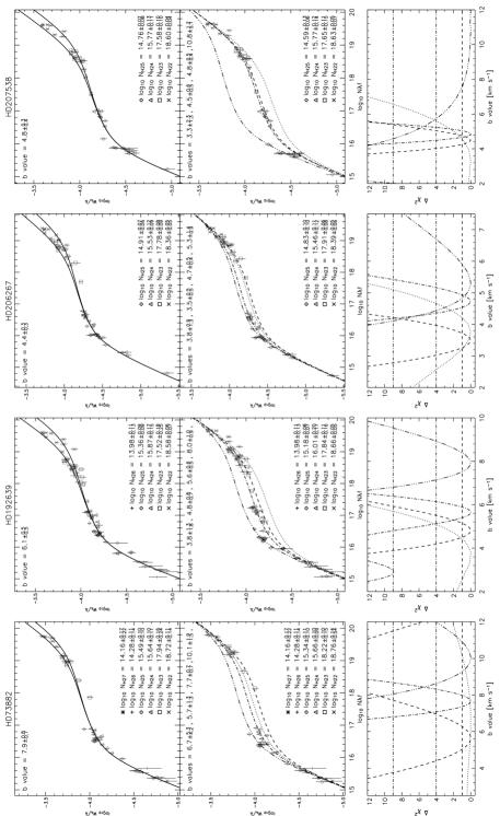
The best COG fits are shown in Figure 1. The upper plots show the resulting COG using a single $b$ value for all the rotational levels. The value of $\chi^{2}$ compared to the number of degrees of freedom is the best mathematical tool to evaluate the goodness of a fit. For these fits, the values are 52/35 for HD 73882, 110/58 for HD 192639, 54/44 for HD 206267, and 37/36 for HD 207538. The probabilities of having $\chi^{2}_{\nu}$ equal to or larger than those values are 3$\%$ ($>2\sigma$), 0.0045$\%$ ($>4\sigma$), 14$\%$ ($>1\sigma$) and 42$\%$ respectively. Therefore, the result is not significant for HD 207538 but HD 192639, and to a lesser extent, HD 73882 and HD 206267, clearly have an inconsistency in the fit. The middle plots display our best fits using different $b$ values for each rotational level and the bottom plots show the $\Delta\chi^{2}$ as a function of $b$, again, for each rotational level. All errors listed here are at the 2$\sigma$ level, corresponding to a $\Delta\chi^{2}$ of 4.

To check the possibility that some systematic problem in one (or a few) lines could induce a “false broadening effect” on the HD 192639 dataset, we randomly removed half of our measurements, then the other half. The results, summarized in Table 4, confirm the presence of the broadening.

3.2 Profile Fitting Method

The spectral resolution ($\approx$ 20 km s^-1, varying over several km s^-1, depending on the detector used), is insufficient to directly determine variations in the broadening of lines, which are typically of the order of a few km s^-1. Instead, it is the relative shape of the lines, combined with knowledge of the oscillator strengths, that provides meaningful information. We used a profile fitting routine, Owens (Lemoine et al., 2002; Hébrard et al., 2002), developed by M. Lemoine at the Institut d’Astrophysique de Paris, which allows fitting all the lines simultaneously while considering different $b$ values for each rotational level. To minimize systematic errors induced by the PSF, we allowed the width of the PSF to vary by $\approx$ 25 $\%$ about the nominal value (15-25 km s^-1). An important advantage of fitting multiple species is the added ability to work with semi-blended lines. The lines that were included with this method are listed in Table 3. This was particularly helpful in constraining the $J$ = 2 $b$ value, because of the weak oscillator strength of the 1112.5 Å blended line. Figure 2 shows some sample best fits for the 1017.8 Å ($J$ = 5), 1116.0 Å ($J$ = 4) and 1115.91 Å ($J$ = 3) lines. In Figure 3 we plot the $\Delta\chi^{2}$ for the $b$ values used in the fits. To account for systematic uncertainties, we scaled the errors (by a factor of 1 to 2) so that the $\chi^{2}$ minimum is equal to the number of degrees of freedom (for more on the $\chi^{2}$ technique while using Owens, see Hébrard et al., 2002).

To convince ourselves that profile fitting with a single $b$ value for all levels does not accurately describe our data, we did the fitting for HD 73882 and HD 192639 and compared the fitting on one particular line. The 2 panels in the right column of Figure 4 show the best fit for the 1017.8 Å line (segment LiF1A) when a single $b$ value was used for all rotational levels, while the left panels show the best fits using individual $b$ values. Without taking systematic uncertainties into account (i.e., without scaling the errors), the $\chi^{2}$ for the left panels are close to the number of degrees of freedom (28/27 for HD 73882 and 24/21 for HD 192639), indicating that the fits are reliable. On the other hand the $\chi^{2}$ for the right panels (62/27 and 44/21 respectively) indicate an inconsistency. Note that the PSF was a free parameter and had a value of 2.96 binned pixels (23.4 km s^-1) for HD 73882 and 2.98 binned pixels (23.2 km s^-1) for HD 192639 (left column). For the right column, the obtained PSFs are 2.67 pixels (21.1 km s^-1) for HD 73882 and 2.42 pixels (19.1 km s^-1) for HD 192639. The differences in the PSFs are within the FUSE resolution uncertainties (see Moos et al., 2000).

3.3 Results

Tables 5 list the column densities and the $b$ values, respectively, derived using the methods described above (2$\sigma$ uncertainties). Profile fitting allows us to quickly determine upper limits on column densities for $J$ levels which only have transitions that are too weak to be used with the COG method. Column densities for the $J$ = 0 and 1 levels, for the four stars, are from Rachford et al. (2002). The $b$ values are consistent between PF and COG. In each case, but with different reliability levels, the velocity dispersion shows the same increasing trend with the H₂ excitation levels. Since $b$ values and column densities are interdependent, it is an important result for observers investigating saturated H₂ lines. If the broadening of the higher $J$ levels is assumed to be equal to those of the lower $J$ levels, then there is the possibility of considerably overestimating the column densities.

4 On the source of excitation and broadening

In light of the results presented above a question must then be asked: What causes the increase in the broadening of the H₂ lines with increasing $J$ level? An obvious explanation would be that we may have a broad component revealed at high rotational level by an high excitation temperature. To test this possibility, we plot in Figure 5 the curves of growth for a sightline having two components with different velocity dispersions. Because the relative strength differs from one rotational level to the other, each level correspond to a curve of growth with a different shape. As an example, we used the excitation diagram of target HD 193639 to fit two components which are associated with the $J=2$ level for one, and the $J=5$ level for the other. We then fitted the EqWs on the COGs of their corresponding excitation level. The fit explain why an effect due to the variation in the ratio between two components, one broad and the other narrower, can be seen as a variation in the broadening. We note nevertheless that this explanation is incompatible with Component 1 observed with IMAPS towards $\zeta$ Ori A (Jenkins & Peimbert, 1997). In this case, the third rotational level column density is so low, that it cannot belong to a different component.

Finding an explanation for the presence of a broad component is another challenge. It may be the key behind the source of both the excitation of H₂ and the presence of large amounts of CH⁺. Specifically, the fast ion-molecule reaction, CH⁺ + H₂ $\longrightarrow$ CH${}_{2}^{+}$ + H, in cold gas, predicts CH⁺ column densities far below the observed levels (Watson, 1974). This is also the case toward our sightlines ($N({\rm CH^{+}})>10^{13}$ cm^-2). The solution might be in warm interstellar gas ($T\geq 10^{3}$ K) in which the endothermic reaction C⁺ + H₂ $\longrightarrow$ CH⁺+ H - 0.4eV can provide an equilibrium density close to the observed levels. The presence of a warm component received strong support by the observation of a correlation between CH⁺ and the rotationally excited H₂ (Lambert & Danks, 1986). However, since until now no direct observations of this warm component have been obtained, parameters such as its density and temperature are unknown. The increase of $b$ with increasing $J$ level seems to be direct evidence of a warm component. Several excitation mechanisms, discussed below, could be responsible for this effect.

4.1 UV-pumping

The ro-vibrational cascading releases its energy through infrared photons (Black & Dalgarno, 1976). Like photoexcitation, such energy loss does not change the kinetic energy of the molecules, and therefore it does not affect the velocity dispersion. Heating of the gas can nevertheless occur, through photodissociation of H₂ and photoelectron emission from dust grains. However, such process would require a high UV field (as the one towards the Pleiades cluster, e.g. White, 1984), and is an unlikely explanation for a broadening of up to 10 km s^-1.

4.2 H₂-formation pumping

When molecules are created on the surface of grains, they carry away most of the initial energy ($\approx$ 4.5 eV) which provides the kinetic, rotational and vibrational excitation of H₂. Support for this mechanism was obtained by Wagenblast (1992) who calculated the column density ratio between the $J$ = 4 to 7 levels in good agreement with observations. However, absolute column density calculations do not exist. To address this, we constructed a time-dependent model in which we followed the stochastic evolution of the molecules after their grain formation. Details of the model are given in the Appendix. According to this model, dispersions appear as a natural consequence of the equilibrium among the various excitation and decay processes. Figure 6 shows the expected broadening, as a function of the density and the rotational level. Using the expected broadening in conjunction with Equation A3 we are able to calculate the densities and formation rates needed to explain both the velocity dispersions and the column densities of the broader rotational levels ($J\geq 4$). The densities are in agreement with previous analysis of the C I fine-structure excitation for HD 192639 and HD 206267, which led to to estimated densities of 16 cm^-3 (Sonnentrucker et al., 2002) and 30 cm^-3 (Jenkins & Tripp, 2001), respectively. However, the formation rates implied by our models ($R$ in Table 6), do not agree with previously calculated values ($R\approx 3\times 10^{-17}$ cm³ s^-1 in Jura, 1975; Gry et al., 2002). There is a factor of approximately ten between the rate needed to explain the column densities and the rates mentioned above.

A second argument against H₂-formation pumping as responsible for the broadening of the excited states comes from the difficulty to account for the CH⁺ column density. We report on the upper right panel of Figure 7 the threshold energy for the C⁺+H₂ reaction, and found that the time during which the molecule is kinetically warm is $t_{\rm warm}=4\times 10^{9}/n$ s (the cooling time is roughly inversely proportional to the density $n$, in cm^-3). Assuming that the density is spatially uniform along the sightline, we can obtain the column density of warm H₂ as a function of the atomic hydrogen and the formation rate : $N({\rm H_{2}})_{\rm warm}=N({\rm H})\,nR\,t_{\rm warm}$. Considering the formation rates from Table 6, we obtain a ratio $N({\rm H_{2}})_{\rm warm}/N({\rm H})\approx 1.2\times 10^{-7}$, a value several orders of magnitude below what is needed to explain the column density of CH⁺ ($N({\rm H_{2}})_{\rm warm}/N({\rm H_{2}})_{\rm cool}\approx 10^{-3}$ in Lambert & Danks, 1986).

4.3 Collisional excitation in a warm environment

Warm low density interstellar gas surely is present along the lines of sight. Field et al. (1969) were the first to show that warm gas could be thermally stable at low densities. Such gas ($n_{\rm H}\approx 0.1$ cm^-3; $T\approx 7000$ K) appears to be the major constituent – in mass – of the local interstellar cloud (Frisch & York, 1983; Linsky, 1996; Lallement, 1998), but a recent survey of the LISM, performed by Lehner et al. (2003), showed that in this medium, the H₂ molecular fraction is low, close to 10^-5. The problem appears to be that at such densities and temperatures, H₂ formation on grains becomes negligible. Other routes exist, such as formation through hydrogen ions (Black et al., 1981), but the rates for the process are low, as is the observed amount of such ions (Andre et al., 2002). The same arguments can be used against the presence of H₂ in the warm postshock gas of dissociative shocks. However, Jenkins & Peimbert (1997) concluded anyway that in the line of sight towards $\zeta$ Ori A, the dispersion of the $J=5$ line could be the trace of an ongoing J-type shock after which the gas recombines and cools. It is true that this theory was corroborated by a shift of the line centers - the higher $J$ levels being shifted towards lower velocities - which is difficult to explain otherwise.

But shifts could also be the trace of slower shocks, C-type shocks. Even though the conditions in the postshock gas are not favorable in terms of H₂ formation, the fact that it is non-dissociative makes it possible to contain a large amount of heated H₂. Hence, Elitzur & Watson (1978) showed that such shocks could heat a large portion of the cloud with temperatures of several thousands Kelvin. This mechanism would generate both the broadening and the CH⁺ column densities. However, there are several arguments against the presence of a single important shock front: predictions of $N$(OH) produced via an endothermic reaction would be significantly higher than what is observed, and significant velocity shifts required for this type of shocks are usually undetected. We can however derive the environment parameters in the hypothesis of a thermal broadening of the postshock gas. We listed in Table 7 the kinetic temperature (under the assumption that the linewidths are mostly due to thermal broadening), and the excitation temperature (derived from the $J=5$ and 7 levels) for the four lines of sight. The difference between the two temperatures constrain the ratio between collisional excitation and radiative de-excitation rates. Hence, we used the rates from Le Bourlot et al. (1999) and Wolniewicz et al. (1998) to infer the densities, and therefore the pressure $log(P/k)=log(nT)$. We note that we are not able to derive lower limits of the $J=7$ rotational column density. However, we used the best fitting values to infer the pressure of the neutral gas, and obtained values significantly higher than those derived from the C I fine structure; log(P/k) $\approx 3.1$ for HD 192639 (Sonnentrucker et al., 2002) and 3.5 for HD 206267 (Jenkins & Tripp, 2001).

From the pressure calculations, we argue that we are more likely in the presence of material cooler than what can be derived from a thermal velocity dispersion. The molecule must still be hot enough to explain the excitation temperature (approximatively a thousand Kelvin), but not up to the temperature required for a thermal broadening ($T^{k}$ in Table 7). Hence, the only remaining explanation of the velocity dispersion is that we are looking at a warm and turbulent layer, most probably intimately associated with the cold medium. To explain the presence of such layer, some invoke supra-thermal velocities of ions relative to the neutrals driven by multiple magneto-hydrodynamic (MHD) criss-crossing shocks (Gredel et al., 2002). Others invoke the intermittency of turbulence and the existence of localized tiny warm regions, transiently heated by bursts of ion-neutral friction and viscous dissipation in coherent and intense small small vortices (Joulain et al., 1998). The main physical difference between each phenomenon is the thickness and the crossing time. While a warm MHD postshocks layer can have a thickness of $\approx 0.1$ pc, coherent vortices threaded by magnetic fields may have radii as small as $\approx 20$ AU. Both would achieve peak temperature around 1000K, but with differential velocities around 10 km s^-1 for the MHD shocks and around 4 km s^-1 in a coherent vortice.

Towards our targets, the situation would be perfectly describe by both explanations. The many small-scale shocks or vortices would create the observed velocity dispersion, while embedded magnetic fields would generate differential velocities between ion and neutral species, reacting into CH⁺ through the C⁺ + H₂ $\longrightarrow$ CH⁺+ H endothermic reaction. It would also give an answer to multiple quests for a warm layer (e.g. CO, HCO+, H₂O in Pety & Falgarone, 2000; Liszt & Lucas, 2000; Neufeld et al., 2002). However, other heating process may be possible, and are difficult to rule out due to our low spectral resolution. The probability distribution functions of these high rotational levels — either in FUV or IR (Verstraete et al., 1999, Falgarone et al. in press) — would eventually help us to distinguish between one process and the other.

5 Summary

We observed four highly reddened ($E_{(B-V)}\approx 0.6$) lines of sight in which the saturation of the higher rotational levels of H₂ allows us to infer their velocity dispersion. We measured broadenings up to 10 km s^-1, increasing with the energy of the rotational level. Considering the fact that it was already observed towards several other sightlines (Spitzer & Cochran, 1973; Spitzer et al., 1974; Jenkins & Peimbert, 1996), we suggest that this phenomenon is a fairly common one. As a first result, we suggest caution in investigating saturated H₂ lines since assuming an identical linewidth for all the rotational levels could lead to significant systematic errors on the column densities.

We looked at the possible sources of rotational excitation to see which could induce such broadening of the absorption lines. We ruled out UV-pumping which can not create a velocity dispersion by itself. We constructed a time dependent model of the state of the molecule following formation on the grain. From it, we deduced that such mechanism may be responsible for the broadening, but would however need a formation rate ten times the one derived from previous studies (Jura, 1975). We also note that the amount of warm H₂ created would not be enough to account for the observed column densities of CH⁺.

We conclude that the more likely explanation is the presence of a turbulent, warm layer in the molecular cloud. The temperature would need to be over 600 K to account for the rotationally excited H₂, and the velocity dispersion of the gas patches around 8 km s^-1. Small criss-crossing shocks or vortices could be the phenomenon behind this turbulent layer. Magneto-hydrodynamic waves created inside them would convert the kinetic energy to create the observed amount of CH⁺ through its endothermic reaction with H₂.

Appendix A Modeling H₂ formation

A.1 Description

In this section we describe our numerical model of H₂ excitation and de-excitation following H₂ formation on grains. We use it to show the existence of a possible correlation between the excitation level of the molecule and the line broadening associated with that level. We also use it to calculate the amount of excited H₂ obtained from H₂-formation pumping. Note that throughout most of this section we are dealing only with the gas that is excited by formation pumping. The effects described here are not affected by the presence of another gas component (at the same level) excited by a different mechanism.

The formation of H₂ on grains has been discussed at length in the literature (e.g. Gould & Salpeter, 1963; Knaap et al., 1966; Augason, 1970; Hollenbach & Salpeter, 1971; Lee, 1972). Our model is based on the fact that when H₂ molecules are formed, they will leave the surface of the grain carrying with them excess energy, which will be distributed as surface, kinetic, rotational and vibrational energy. If we can determine the cross-sections for the various processes by which the molecules either lose or convert energy from one form into another, we can then estimate the average kinetic energy over the lifetimes of each species. Adding in the formation rates, we are able to predict the column density and velocity dispersion of each level.

A.1.1 Initial distribution

Recent simulations of H₂ formation have been performed for graphite surfaces (Parneix & Brechignac, 1998; Meijer et al., 2001) and icy interstellar dust (Takahashi et al., 1999). In all cases, the molecules leave the grain with an initial energy of 4.48 eV, but the distribution among binding, kinetic, and rotational energy differ considerably. We based our model on the quasi-classical computer simulation of the Parneix & Brechignac paper, due to their choice of computational method and physical model, which includes an entrance-channel barrier on the potential energy surface of the grain. The initial distribution over the vibrational levels corresponds to Fig. 11 of their paper, and averages around 1.1 eV, with a peak at $v$ = 0. The distribution of rotational energy, with a mean value of 0.7 eV, corresponds to the Fig. 9 from the same paper, and is the same for each vibrational level. 1.7 eV is carried as kinetic energy, and the remainder is used to desorb the molecule from the grain. The implications of these choices are discussed in the “Model results & considerations” Section. The ortho/para repartition (OPR) is an important factor in the column density calculations, but fortunately, it does not affect the results concerning the velocity dispersions. In view of the results of Persson & Jackson (1995), we decided not to include the statistical weight factor of 1/3.

A.1.2 Kinetic cooling

Starting with an initial kinetic energy, the H₂ molecule will cool down, while interacting with its environment. Because the formation rate is proportional to the density of atomic hydrogen, most of the formation of molecular hydrogen takes place in the photodissociation region, where hydrogen is mostly atomic. Moreover, simulations (Le Petit et al., 2002) show a sharp decrease of the molecular fraction as we go deeper in the cloud, implying a formation rate only marginal inside the cloud. It leaded us to approximate the formation environment as being purely atomic. Under this assumption, we needed just three parameters to compute the kinetic cooling: the H-H₂ cross-section ($\sigma$), the mean energy loss per collision ($\gamma$), and the density ($n$). While $n$ is just a property of the medium, the two other parameters depend on the energy of the molecule. To obtain $\sigma$, we extrapolated to higher energies the values in Fig. 2 of Clark & McCourt (1995). The results are plotted in the upper left panel of Figure 7. $\gamma$ was generated using equations (12) and (25) in Kharchenko et al. (1998), while $n$ is left as a free parameter, varying from 0.1 to 1000 cm^-3. The right upper panel of Figure 7 displays the estimated kinetic energy as a function of time for a medium with density $n=10$ cm^-3. One can see that the translational energy is lost fairly slowly, allowing time for the molecule to undergo endothermic reactions. For example, if we consider the threshold energy for the C⁺ + H₂ $\longrightarrow$ CH⁺+ H - 0.4eV reaction (dashed line), the molecule would have such or more energy during $t_{warm}=4\times 10^{8}$ seconds ($\approx 10$ ans).

A.1.3 Radiative cooling

From the initial distributions, we generated a table of 20 rows (corresponding to the 20 first rotational levels) and 7 columns (corresponding to the 7 first vibrational levels). In steps of 10⁵ seconds, and using the radiative decay table from Wolniewicz et al. (1998), we computed the density of each excitation level from its formation until 3.5 $\times$ 10¹¹ seconds. The panel in the center of Figure 7 shows the densities (normalized to 1) of each vibrational level (independent of the rotational level). After a fairly short time ($\approx 10^{7}$s), all of the molecular hydrogen is in the ground vibrational state. Then, the model clearly shows the progression towards lower $J$ levels as time increases (lower panels of Figure 7). The rising parts of the density curves are caused by the cascading down from higher $J$ or $v$ levels, while the steep drops occur at the radiative lifetime. Interestingly, these lifetimes (e.g., A${}_{42}^{-1}\approx 10^{9}$ s) are of the order of the kinetic cooling time (see previous paragraph). It follows that, depending on the density of the cloud, some rotational levels will be kinetically hot, while lower levels will not.

A.1.4 Inelastic collisional cooling & excitation

In addition to the decay rates, collisional excitation and de-excitation may have an important effect, especially while the molecule is still highly energetic, or when the density is high. We used the rates from the web site http://ccp7.dur.ac.uk/cooling_by_h2/index.html (Forrey et al., 1997; Le Bourlot et al., 1999), in addition to the decay rates of the above section, to model the time dependent density distribution. The lower panels of Figure 7 show the resulting densities (normalized to 1) of the pure rotational levels. The specific conditions for this plot are a density of 10 particles per cm³, and an ambient temperature of 100 K. As discussed in the previous paragraph, it is apparent that the fraction of each excited state falls off rapidly at a time corresponding to the decay rate, and that inelastic collisions are not an important de-excitation mechanism. Numerical tests show that for densities below several hundred cm^-3, inelastic collisions are negligible compared to radiative decay.

A.2 Model results & considerations

Integrating the normalized column densities over time allows us to extract two pieces of information :

1. The mean kinetic energy of each rotational levels, which can be directly linked to the velocity dispersion as long as we assume that the excitation is mainly due to its formation on the grain. The mean energy is obtained by:

   $$E_{k}(J,n)=\frac{\int^{+\infty}_{0}\mathrm{Density}(J,n,t)\times E(t)dt}{\int^{+\infty}_{0}\mathrm{Density}(J,n,t)dt}$$ (A1)

   In practice the upper limit of the integration was set to 3.5 $\times 10^{11}$ seconds, by which time the excited species have largely decayed. The velocity dispersion, i.e., the broadening, is therefore

   $$b=\sqrt{4/3*E_{k}/(2m_{\rm H})}\,.$$ (A2)

   We plotted in Figure 6, the broadening of each rotational levels between 2 and 6, clearly showing that it is increasing with the rotational level. Again, this is only the case when the species are populated by H₂-formation pumping. The broadening of higher rotational levels ($J=4$ and 5) were fitted on the curves, and estimated densities are reported for our four targets in Table 6.

2. Still assuming no other source of excited H₂, we are also able to calculate the molecular hydrogen column densities of the excited levels. The densities depend on the formation rate ($nR$), and the atomic hydrogen density. Assuming that the density is spatially uniform along the line of sight, we can use the column density of atomic hydrogen $N(\rm H)$, and therefore, have the following equation:

   $$N({\rm H_{2}})(J,n)=N({\rm H})\,nR\,\int^{+\infty}_{0}\mathrm{Density}(J,n,t)dt$$ (A3)

   To remove the effect of the formation OPR on the column density, we considered the sum of the column densities of the $J=4$ and 5 levels. The formation rates needed to create such column densities are reported in Table 6.

The distribution of the formation-energy of H₂ has been calculated through many other theoretical models, yielding quite different results in all the different parameters. Two parameters have a large influence on our results: the initial kinetic and rotational energies. On one hand, the kinetic energy will decide the amplitude of the velocity dispersion. For instance, whereas our model starts with a kinetic energy of 1.7 eV, Meijer et al. (2001) find an initial energy of 1.18 eV which would scale down all our broadening calculations by a factor of 1.2. More specifically, from Equation A2, a broadening of 8 km s^-1 can be explained if the kinetic initial energy is equal or above 0.95 eV. This is compatible with most but a few of the theoretical formation models. On the other hand, the initial rotational energy does constrain the calculated column density of the rotational levels. Because the radiative lifetimes of the higher levels are significantly smaller than that of the lower rotational levels, a first approximation can be that each level is populated by its initial population plus the initial population of the higher level. Therefore, any model yielding an average initial rotational energy above 0.4 eV would give similar column density results for $J\leq 7$. Except for Duley & Williams (1986), most of the theoretical models agree with a rotationally hot initial distribution, hence in accordance with our chosen model.

Figure 1: Curve of growth analysis for H₂ along the HD 73882, HD 192639, HD 206267 and HD 207538 lines of sight. The plots at the top assume a common $b$-value for all $J$ levels. In the middle plots, each $J$ level is fit with a different $b$-value. The plots in the bottom of the figure present $\Delta\chi^{2}$ as a function of $b$ for the COGs displayed in the middle of the figure. In the $\Delta\chi^{2}$ plots, the different rotational levels are represented with dotted ($J$ = 2), dashed ($J$ = 3), dot-dashed ($J$ = 4), and dot-dot-dot-dashed ($J$ = 5) lines. Note that due to the non-linearity of the COG, the $\Delta\chi^{2}$ sometimes shows two minima. In these cases, the second minimum is ruled out on the grounds that the resulting column densities are not physical.

Figure 2: Best profile fits to the $J=5$ 1017.8 Å line (left) and $J=3$ 1115.9 Å and $J=4$ 1116.0 Å lines (right), for the four sightlines. Each rotational level is fit with a different $b$ value. The continuum is normalized to 1.

Figure 3: $\Delta\chi^{2}$ curves for the different $b$ values used with profile fitting. The different rotational levels are represented with dotted ($J$ = 2), dashed ($J$ = 3), dot-dashed ($J$ = 4), and dot-dot-dot-dashed ($J$ = 5) lines.

Figure 4: Best profile fits of the $J=5$ 1017.8 Å line for HD  73882 (top) and HD  192639 (bottom) using a single $b$ value for all $J$ levels (right) and allowing different $b$ values for each $J$ level (left). The inadequacy of the single $b$ value fits for all $J$ levels is apparent both from close inspection of the fits and from the reduced $\chi^{2}$ values (see section 3.2).

Figure 5: Left panel : Excitation diagram of the H₂ along the HD 192639 line of sight. We fitted the column densities with several components, with different excitation temperatures and velocity dispersions. The $T_{ex}=T_{J=2-4}$ component is supposed to have a broadening equal to the $J=2$ species, and the $T_{ex}=T_{J=5-7}$ component a broadening equal to the $J=5$ species. Right panel : Two components curve of growth for $J=2$ to 6, with a relative strength in accordance with the two components fitted on the higher levels of the excitation plot. A variation of the $b$-values appear due to the presence of the two components.

Figure 6: Line broadening ($b$) derived from the mean kinetic energy of each level following formation on a grain. Since the value of the kinetic energy is dominated by collisional cooling, the broadening is a strong function of the density ($n$). The thin vertical lines show the density towards HD 192639 (Sonnentrucker et al., 2002) and HD 206267 (Jenkins & Tripp, 2001).

Figure 7: Time dependent model of molecular hydrogen following formation on grains (see Appendix). Upper left panel : Effective H-H₂ cross-section as a function of the kinetic energy. Upper right panel : Kinetic energy of the H₂ molecule as a function of time. The dashed line corresponds to the energy threshold from which C⁺ can react with H₂ to form CH⁺. Three lower panels : Distribution of H₂ molecules over the vibrational and the ortho and para rotational states, as a function of the molecule’s lifetime. Note that radiative vibrational transitions ensure decay towards the vibrational ground state on short time scales. The initial rise of the rotational density curves is due to the cascading of molecules down from the higher $J$ and $V$ levels, whereas the steep drops occur at the radiative lifetime of the level. Because collisional excitation and de-excitation are part of our simulation, all these plots depend on the density, here equal to 10 cm^-3.

Table 1: Sightline and Stellar Properties

Star	l (∘)	b (∘)	V (mag)	E${(B-V)}$	AV	Sp.T.
HD 73882	259.83	+0.47	7.27	0.72	2.28	O9III
HD 192639	74.90	+1.48	7.11	0.66	1.87	O8e
HD 206267	98.98	+3.71	5.62	0.52	1.37	O6e
HD 207538	102.86	+6.92	7.30	0.64	1.43	B0V

Table 2: Log of FUSE Observations

Star	FUSE ID	Observation	Number of	Exposure Time	S/N
		Date	Exposures	(Ks)
HD 73882	P1161301	2000.01.24	6	11.9	5.1
..	P1161302	2000.03.19	8	13.6	4.6
HD 192639	P1162401	2000.06.12	2	4.8	8.1
HD 206267	P1162701	2000.07.21	3	4.9	10.2
HD 207538	P1162902	1999.12.08	4	7.7	6.2
…	P1162903	2000.07.21	10	11.2	7.1

Table 3: H₂ equivalent width measurements

Species	$\lambda$ (Å)	log ($f\lambda$)	HD 73882 Wλ(mÅ)	HD 192639 Wλ(mÅ)	HD 206267 Wλ(mÅ)	HD 207538 Wλ(mÅ)
H2 $J$ = 2…..	941.606	0.498	…	111.4 $\pm$ 9.7	88.3 $\pm$ 8.0	…
	957.660	0.661	…	148.1 $\pm$ 13.5	115.1 $\pm$ 6.1	147.6 $\pm$ 13.6
	975.351	0.810	…	151.1 $\pm$ 11.0	124.9 $\pm$ 6.7	144.7 $\pm$ 10.3
	1005.40	0.998	…	212.9 $\pm$ 11.5	162.4 $\pm$ 7.7	208.1 $\pm$ 10.8
	1016.47	1.016	323.6 $\pm$ 33.3	245.6 $\pm$ 12.7	183.2 $\pm$ 8.4	229.1 $\pm$ 10.1
	1040.37	1.030	359.7 $\pm$ 31.9	275.7 $\pm$ 13.5	202.9 $\pm$ 8.8	263.6 $\pm$ 13.5
	1053.29	0.980	283.0 $\pm$ 23.6	273.5 $\pm$ 13.1	193.7 $\pm$ 9.3	270.1 $\pm$ 13.6
	1066.91	0.881	280.5 $\pm$ 23.9	257.7 $\pm$ 11.6	192.9 $\pm$ 9.2	239.7 $\pm$ 10.4
	1081.27	0.709	256.5 $\pm$ 24.9	200.1 $\pm$ 11.0	162.8 $\pm$ 6.9	202.6 $\pm$ 11.4
	1096.45	0.417	220.1 $\pm$ 27.4	175.1 $\pm$ 8.5	PF	PF
	1112.51	-0.111	PF	PF	PF	PF
H2 $J$ = 3…..	934.800	0.820	…	106.3 $\pm$ 9.3	…	…
	942.970	0.729	…	108.5 $\pm$ 14.2	85.2 $\pm$ 8.5	…
	944.337	0.519	…	95.2 $\pm$ 13.9	67.5 $\pm$ 9.4	…
	958.953	0.930	…	95.8 $\pm$ 8.6	97.5 $\pm$ 6.5	90.8 $\pm$ 7.7
	960.458	0.674	…	92.7 $\pm$ 8.5	90.5 $\pm$ 6.8	86.7 $\pm$ 5.9
	995.974	1.218	…	143.9 $\pm$ 9.6	117.6 $\pm$ 8.3	109.2 $\pm$ 6.6
	997.830	0.942	…	123.1 $\pm$ 11.9	97.5 $\pm$ 9.4	91.4 $\pm$ 8.9
	1006.42	1.199	PF	PF	PF	PF
	1017.43	1.270	PF	PF	PF	PF
	1019.51	1.030	195.0 $\pm$ 16.4	116.0 $\pm$ 6.9	113.1 $\pm$ 7.2	101.8 $\pm$ 4.5
	1028.99	1.250	…	144.9 $\pm$ 10.4	…	128.2 $\pm$ 5.3
	1041.16	1.216	204.0 $\pm$ 12.5	159.3 $\pm$ 9.5	146.3 $\pm$ 7.7	122.9 $\pm$ 6.6
	1043.51	1.052	182.1 $\pm$ 11.1	139.5 $\pm$ 8.1	131.1 $\pm$ 6.6	117.6 $\pm$ 4.8
	1053.98	1.150	216.0 $\pm$ 13.4	159.5 $\pm$ 10.6	137.6 $\pm$ 7.7	131.7 $\pm$ 6.7
	1056.48	1.006	192.8 $\pm$ 12.0	125.6 $\pm$ 6.7	122.6 $\pm$ 7.5	121.6 $\pm$ 5.5
	1067.48	1.028	176.0 $\pm$ 15.7	129.9 $\pm$ 7.6	130.9 $\pm$ 7.4	119.0 $\pm$ 5.3
	1070.15	0.909	196.0 $\pm$ 12.5	134.6 $\pm$ 8.1	129.0 $\pm$ 6.9	110.0 $\pm$ 10.4
	1099.80	0.448	148.0 $\pm$ 13.7	103.1 $\pm$ 5.4	92.1 $\pm$ 6.8	95.2 $\pm$ 3.9
	1112.59	-0.024	PF	PF	PF	PF
	1115.91	-0.081	110.9 $\pm$ 9.2	96.7 $\pm$ 6.3	67.8 $\pm$ 3.7	83.8 $\pm$ 4.0
H2 $J$ = 4…..	935.969	1.264	…	75.2 $\pm$ 6.4	…	…
	979.808	1.095	…	76.7 $\pm$ 7.1	55.2 $\pm$ 3.8	…
	994.234	1.134	…	77.3 $\pm$ 8.5	53.2 $\pm$ 6.2	…
	999.272	1.217	…	88.8 $\pm$ 8.1	54.2 $\pm$ 3.3	59.4 $\pm$ 4.9
	1017.39	1.002	PF	PF	PF	PF
	1032.35	1.247	100.7 $\pm$ 6.4	89.0 $\pm$ 6.1	60.9 $\pm$ 3.1	66.2 $\pm$ 3.0
	1044.55	1.206	91.9 $\pm$ 4.3	86.7 $\pm$ 4.2	…	72.9 $\pm$ 3.6
	1047.56	1.062	93.9 $\pm$ 6.5	79.9 $\pm$ 4.4	54.6 $\pm$ 2.6	64.1 $\pm$ 3.6
	1057.39	1.135	97.0 $\pm$ 4.5	72.8 $\pm$ 4.2	59.9 $\pm$ 4.1	65.8 $\pm$ 3.2
	1060.59	1.019	78.3 $\pm$ 5.3	81.2 $\pm$ 3.9	57.1 $\pm$ 2.8	63.0 $\pm$ 3.4
	1074.32	0.923	91.1 $\pm$ 5.6	71.2 $\pm$ 3.7	51.5 $\pm$ 3.3	57.7 $\pm$ 5.2
	1085.15	0.817	…	70.5 $\pm$ 8.8	45.3 $\pm$ 4.0	…
	1088.80	0.752	78.8 $\pm$ 5.4	71.6 $\pm$ 4.0	46.7 $\pm$ 3.1	58.4 $\pm$ 2.8
	1100.17	0.498	62.5 $\pm$ 4.2	73.2 $\pm$ 5.5	43.6 $\pm$ 3.7	…
	1104.09	0.461	…	64.5 $\pm$ 3.8	…	…
	1116.03	-0.060	34.1 $\pm$ 4.5	44.7 $\pm$ 4.8	17.6 $\pm$ 2.9	28.3 $\pm$ 3.4
	1120.26	-0.069	30.5 $\pm$ 3.0	45.4 $\pm$ 5.9	20.2 $\pm$ 2.5	33.3 $\pm$ 3.1
H2 $J$ = 5…..	942.691	0.765	…	37.5 $\pm$ 8.7	…	…
	974.889	1.138	…	68.4 $\pm$ 6.3	38.8 $\pm$ 3.8	…
	996.129	1.102	…	PF	45.4 $\pm$ 6.3	40.2 $\pm$ 8.0
	997.644	1.110	…	62.3 $\pm$ 6.4	44.5 $\pm$ 4.8	33.3 $\pm$ 10.1
	1006.34	0.940	PF	PF	PF	PF
	1017.01	1.060	88.3 $\pm$ 9.0	67.6 $\pm$ 4.5	PF	PF
	1017.84	1.384	117.6 $\pm$ 7.5	82.0 $\pm$ 3.8	51.4 $\pm$ 3.1	56.4 $\pm$ 5.0
	1040.06	1.074	91.2 $\pm$ 5.4	64.9 $\pm$ 3.4	37.1 $\pm$ 2.7	33.7 $\pm$ 3.6
	1052.50	1.068	80.8 $\pm$ 6.2	64.8 $\pm$ 3.2	38.4 $\pm$ 3.4	30.7 $\pm$ 3.0
	1061.70	1.126	87.8 $\pm$ 12.0	76.8 $\pm$ 3.4	39.1 $\pm$ 2.5	45.4 $\pm$ 4.3
	1065.60	1.026	93.5 $\pm$ 9.2	67.9 $\pm$ 3.6	33.0 $\pm$ 3.2	27.8 $\pm$ 3.2
	1075.25	0.999	94.9 $\pm$ 6.9	70.6 $\pm$ 2.9	36.6 $\pm$ 2.8	31.6 $\pm$ 3.5
	1089.52	0.796	68.9 $\pm$ 4.3	58.1 $\pm$ 4.6	31.2 $\pm$ 3.4	…
	1104.55	0.471	…	30.9 $\pm$ 3.0	…	…
	1109.32	0.467	47.3 $\pm$ 4.1	31.4 $\pm$ 3.1	16.6 $\pm$ 2.0	12.4 $\pm$ 2.2
	1120.41	-0.095	19.3 $\pm$ 3.3	14.7 $\pm$ 2.7	5.0 $\pm$ 0.9	PF
H2 $J$ = 6…..	959.163	1.426	…	16.4 $\pm$ 4.2	…	…
	977.733	1.538	…	20.1 $\pm$ 4.2	…	…
	998.340	1.564	…	22.6 $\pm$ 4.2	…	…
	1019.02	1.318	31.4 $\pm$ 4.9	14.0 $\pm$ 2.4	…	…
	1021.22	1.388	22.7 $\pm$ 6.9	20.2 $\pm$ 3.6	…	…
	1041.74	1.243	26.1 $\pm$ 3.9	11.8 $\pm$ 2.9	…	…
	1045.81	1.076	16.1 $\pm$ 5.1	15.4 $\pm$ 3.5	…	…
	1058.32	1.074	18.0 $\pm$ 3.8	…	…	…
H2 $J$ = 7…..	1060.04	1.193	20.0 $\pm$ 3.9	…	…	…
	1073.00	1.110	14.2 $\pm$ 3.2	…	…	…

Note. — Lines blended but used for profile fitting are noted “PF”. Errors are 1 $\sigma$.

Table 4: COG determined $b$ values for different combinations of EqW towards HD 192639

Level	All the EqW	Half of the EqW	Second half of the EqW
H2 $J$ = 2	$3.8\pm~{}^{1.3}_{2.3}$	$4.3\pm~{}^{2.1}_{2.6}$	$3.3\pm~{}^{2.1}_{2.6}$
H2 $J$ = 3	$4.8\pm~{}^{0.8}_{0.7}$	$5.0\pm~{}^{1.2}_{0.8}$	$4.5\pm~{}^{1.6}_{1.6}$
H2 $J$ = 4	$5.6\pm~{}^{0.6}_{0.5}$	$5.4\pm~{}^{0.6}_{1.1}$	$6.0\pm~{}^{0.7}_{0.8}$
H2 $J$ = 5	$8.0\pm~{}^{1.0}_{0.9}$	$7.8\pm~{}^{2.2}_{1.4}$	$7.9\pm~{}^{1.4}_{1.0}$

Note. — $b$ values are in km s^-1. Errors are 2 $\sigma$.

Table 5: Log column densities and $b$ values obtained with PF and COG for the four lines of sight

$J$ level	HD 73882		HD 192639		HD 206267		HD 207538
cm-2 / km s-1	COG	PF	COG	PF	COG	PF	COG	PF
$N({\rm H}_{2})$ — $J=0$	$20.99\pm~{}^{0.08}_{0.08}$		$20.28\pm~{}^{0.05}_{0.05}$		$20.64\pm~{}^{0.03}_{0.03}$		$20.64\pm~{}^{0.07}_{0.07}$
$N({\rm H}_{2})$ — $J=1$	$20.50\pm~{}^{0.07}_{0.07}$		$20.48\pm~{}^{0.05}_{0.05}$		$20.45\pm~{}^{0.05}_{0.05}$		$20.58\pm~{}^{0.05}_{0.05}$
$N({\rm H}_{2})$ — $J=2$	$18.76\pm~{}^{0.14}_{0.54}$	$19.04\pm~{}^{0.10}_{0.09}$	$18.66\pm~{}^{0.05}_{0.05}$	$18.75\pm~{}^{0.10}_{0.05}$	$18.39\pm~{}^{0.06}_{0.06}$	$18.49\pm~{}^{0.05}_{0.04}$	$18.63\pm~{}^{0.05}_{0.07}$	$18.75\pm~{}^{0.05}_{0.05}$
$N({\rm H}_{2})$ — $J=3$	$18.22\pm~{}^{0.10}_{0.15}$	$18.49\pm~{}^{0.15}_{0.04}$	$17.84\pm~{}^{0.11}_{0.16}$	$18.00\pm~{}^{0.15}_{0.10}$	$17.91\pm~{}^{0.06}_{0.08}$	$17.95\pm~{}^{1.05}_{0.05}$	$17.65\pm~{}^{0.11}_{0.16}$	$17.90\pm~{}^{0.10}_{0.15}$
$N({\rm H}_{2})$ — $J=4$	$15.66\pm~{}^{0.10}_{0.09}$	$15.80\pm~{}^{0.10}_{0.16}$	$16.01\pm~{}^{0.20}_{0.17}$	$15.90\pm~{}^{0.10}_{0.10}$	$15.46\pm~{}^{0.11}_{0.12}$	$15.28\pm~{}^{0.17}_{0.10}$	$15.77\pm~{}^{0.12}_{0.14}$	$15.70\pm~{}^{0.10}_{0.06}$
$N({\rm H}_{2})$ — $J=5$	$15.34\pm~{}^{0.11}_{0.10}$	$15.34\pm~{}^{0.10}_{0.11}$	$15.18\pm~{}^{0.08}_{0.07}$	$15.15\pm~{}^{0.08}_{0.07}$	$14.83\pm~{}^{0.10}_{0.10}$	$14.75\pm~{}^{0.15}_{0.10}$	$14.59\pm~{}^{0.13}_{0.06}$	$14.64\pm~{}^{0.16}_{0.15}$
$N({\rm H}_{2})$ — $J=6$	$14.28\pm~{}^{0.11}_{0.14}$	$14.08\pm~{}^{0.26}_{0.08}$	$13.98\pm~{}^{0.11}_{0.13}$	$14.00\pm~{}^{0.15}_{0.10}$	$\cdots$	$13.84\pm~{}^{0.15}_{?}$	$\cdots$	$13.04\pm~{}^{0.60}_{?}$
$N({\rm H}_{2})$ — $J=7$	$14.16\pm~{}^{0.17}_{0.22}$	$14.08\pm~{}^{0.37}_{0.23}$	$\cdots$	$13.49\pm~{}^{0.35}_{?}$	$\cdots$	$13.59\pm~{}^{0.31}_{?}$	$\cdots$	$13.28\pm~{}^{0.56}_{?}$
$b({\rm H}_{2})$ — $J=2$	$\cdots$	$2.47\pm~{}^{3.0}_{1.7}$	$3.8\pm~{}^{1.3}_{2.3}$	$4.59\pm~{}^{0.40}_{0.70}$	$3.8\pm~{}^{0.9}_{1.3}$	$2.49\pm~{}^{0.20}_{0.40}$	$3.3\pm~{}^{2.3}_{3.3}$	$3.97\pm~{}^{0.20}_{0.20}$
$b({\rm H}_{2})$ — $J=3$	$5.7\pm~{}^{1.3}_{1.3}$	$4.39\pm~{}^{0.4}_{0.2}$	$4.8\pm~{}^{0.8}_{0.7}$	$5.14\pm~{}^{0.20}_{0.20}$	$3.5\pm~{}^{0.5}_{0.5}$	$3.10\pm~{}^{0.30}_{0.10}$	$4.5\pm~{}^{0.6}_{0.5}$	$4.41\pm~{}^{0.20}_{0.20}$
$b({\rm H}_{2})$ — $J=4$	$7.7\pm~{}^{0.7}_{0.7}$	$7.19\pm~{}^{0.4}_{0.3}$	$5.6\pm~{}^{0.6}_{0.5}$	$5.89\pm~{}^{0.20}_{0.30}$	$4.7\pm~{}^{0.5}_{0.4}$	$5.02\pm~{}^{0.15}_{0.45}$	$4.8\pm~{}^{0.5}_{0.4}$	$4.78\pm~{}^{0.20}_{0.30}$
$b({\rm H}_{2})$ — $J=5$	$10.1\pm~{}^{1.9}_{1.5}$	$11.09\pm~{}^{1.2}_{1.0}$	$8.0\pm~{}^{1.0}_{0.9}$	$8.34\pm~{}^{0.80}_{0.40}$	$5.3\pm~{}^{1.5}_{0.9}$	$6.50\pm~{}^{0.60}_{1.40}$	$10.8\pm~{}^{1.2}_{5.1}$	$7.22\pm~{}^{2.40}_{1.60}$

Note. — $J=$ 0 & 1 column densities from Rachford et al. (2002). Errors are 2 $\sigma$.

Table 6: Gas Densities and H₂ Formation rates — $b$ due to H₂-formation pumping

	$n$	$nR$	$R$
Lines of Sight	[cm-3]	[s-1]	[cm3 s-1]
HD 73882	$5\pm~{}^{3}_{?}$	$9\pm~{}^{8}_{4}\times 10^{-15}$	$1.8\pm~{}^{?}_{1.2}\times 10^{-15}$
HD 192639	$13\pm~{}^{5}_{6}$	$4\pm~{}^{5}_{3}\times 10^{-15}$	$3.1\pm~{}^{9.8}_{2.5}\times 10^{-16}$
HD 206267	$25\pm~{}^{11}_{6}$	$6\pm~{}^{4}_{3}\times 10^{-15}$	$2.4\pm~{}^{2.9}_{2.1}\times 10^{-16}$
HD 207538	$13\pm~{}^{20}_{?}$	$3\pm~{}^{2}_{2}\times 10^{-15}$	$2.3\pm~{}^{?}_{1.9}\times 10^{-16}$

Note. — Densities and formation rates come from our measurements reported in Table 5 and model results plotted in Figure 7.

Table 7: Temperatures and Densities — $b$ due to thermal scattering

	$T^{k}$	$T^{ex}_{J=5-7}$	$n$	$log_{10}(P/k)$
Lines of Sight	(K)	(K)	(cm-3)	(log(K cm-3))
HD 73882	$9500\pm~{}^{600}_{600}$	$670\pm~{}^{180}_{100}$	$31\pm~{}^{30}_{14}$	$4.3\pm~{}^{0.4}_{0.3}$
HD 192639	$8200\pm~{}^{400}_{300}$	$500\pm~{}^{120}_{?}$	$13\pm~{}^{17}_{?}$	$3.8\pm~{}^{0.5}_{?}$
HD 206267	$7000\pm~{}^{600}_{700}$	$680\pm~{}^{220}_{?}$	$49\pm~{}^{54}_{?}$	$4.5\pm~{}^{0.4}_{?}$
HD 207538	$8500\pm~{}^{800}_{1700}$	$610\pm~{}^{400}_{?}$	$27\pm~{}^{75}_{?}$	$4.2\pm~{}^{0.8}_{?}$

Note. — $T^{k}$ is the temperature obtained from the formula $b=\sqrt{2kT/m}$. $T^{ex}_{J=5-7}$ is the excitation temperature from the rotational levels 5 and 7.

References

- Andre et al. (2002) Andre, M. K., Désert, J. M., Ehrenreich, D., Ferlet, R., Hébrard, G., Lacour, S., LePetit, F., Leboutei, V., Oliveira, C., & Sonnentrucker, P. 2002, American Astronomical Society Meeting, 201, 0
- Augason (1970) Augason, G. C. 1970, ApJ, 162, 463+
- Black & Dalgarno (1976) Black, J. H. & Dalgarno, A. 1976, ApJ, 203, 132
- Black & Dalgarno (1977) —. 1977, ApJS, 34, 405
- Black et al. (1981) Black, J. H., Porter, A., & Dalgarno, A. 1981, ApJ, 249, 138
- Clark & McCourt (1995) Clark, G. B. & McCourt, F. R. W. 1995, Chem. Phys. Lett., 236, 229
- Duley & Williams (1986) Duley, W. W. & Williams, D. A. 1986, MNRAS, 223, 177
- Elitzur & Watson (1978) Elitzur, M. & Watson, W. D. 1978, ApJ, 222, L141
- Field et al. (1969) Field, G. B., Goldsmith, D. W., & Habing, H. J. 1969, ApJ, 155, L149+
- Forrey et al. (1997) Forrey, R. C., Balakrishnan, N., Dalgarno, A., & Lepp, S. 1997, ApJ, 489, 1000+
- Frisch & York (1983) Frisch, P. C. & York, D. G. 1983, ApJ, 271, L59
- Gould & Salpeter (1963) Gould, R. J. & Salpeter, E. E. 1963, ApJ, 138, 393+
- Gredel et al. (2002) Gredel, R., Pineau des Forêts, G., & Federman, S. R. 2002, A&A, 389, 993
- Gry et al. (2002) Gry, C., Boulanger, F., Nehmé, C., Pineau des Forêts, G., Habart, E., & Falgarone, E. 2002, A&A, 391, 675
- Hébrard et al. (2002) Hébrard, G., Lemoine, M., Vidal-Madjar, A., Désert, J.-M., Lecavelier des Étangs, A., Ferlet, R., Wood, B. E., Linsky, J. L., Kruk, J. W., Chayer, P., Lacour, S., Blair, W. P., Friedman, S. D., Moos, H. W., Sembach, K. R., Sonneborn, G., Oegerle, W. R., & Jenkins, E. B. 2002, ApJS, 140, 103
- Hollenbach & Salpeter (1971) Hollenbach, D. & Salpeter, E. E. 1971, ApJ, 163, 155+
- Horne (1986) Horne, K. 1986, PASP, 98, 609
- Jenkins & Peimbert (1996) Jenkins, E. B. & Peimbert, A. 1996, Bulletin of the American Astronomical Society, 28, 833
- Jenkins & Peimbert (1997) —. 1997, ApJ, 477, 265
- Jenkins & Tripp (2001) Jenkins, E. B. & Tripp, T. M. 2001, ApJS, 137, 297
- Joulain et al. (1998) Joulain, K., Falgarone, E., Des Forets, G. P., & Flower, D. 1998, A&A, 340, 241
- Jura (1975) Jura, M. 1975, ApJ, 197, 575
- Kharchenko et al. (1998) Kharchenko, V., Balakrishnan, N., & Dalgarno, A. 1998, J. Atmos. Sol. Terr. Phys., 60, 95
- Knaap et al. (1966) Knaap, H. F. P., van den Meijdenberg, C. J. N., Beenakker, J. J. M., & van de Hulst, H. C. 1966, Bull. Astron. Inst. Netherlands, 18, 256+
- Lallement (1998) Lallement, R. 1998, Lecture Notes in Physics, v.506, Berlin Springer Verlag, 506, 19
- Lambert & Danks (1986) Lambert, D. L. & Danks, A. C. 1986, ApJ, 303, 401
- Le Bourlot et al. (1999) Le Bourlot, J., Pineau des Forêts, G., & Flower, D. R. 1999, MNRAS, 305, 802
- Le Petit et al. (2002) Le Petit, F., Roueff, E., & Le Bourlot, J. 2002, A&A, 390, 369
- Lee (1972) Lee, T. J. 1972, Nature Physical Science, 237, 99+
- Lehner et al. (2003) Lehner, N., Jenkins, E. B., Gry, C., Moos, H. W., Chayer, P., & Lacour, S. 2003, ApJ, 595, 858
- Lemoine et al. (2002) Lemoine, M., Vidal-Madjar, A., Hébrard, G., Désert, J.-M., Ferlet, R., Lecavelier des Étangs, A., Howk, J. C., André, M., Blair, W. P., Friedman, S. D., Kruk, J. W., Lacour, S., Moos, H. W., Sembach, K., Chayer, P., Jenkins, E. B., Koester, D., Linsky, J. L., Wood, B. E., Oegerle, W. R., Sonneborn, G., & York, D. G. 2002, ApJS, 140, 67
- Linsky (1996) Linsky, J. L. 1996, Space Science Reviews, 78, 157
- Liszt & Lucas (2000) Liszt, H. & Lucas, R. 2000, A&A, 355, 333
- Meijer et al. (2001) Meijer, A. J. H. M., Farebrother, A. J., Clary, D. C., & Fisher, A. J. 2001, J. Chem. Phys., 105, 3359
- Moos et al. (2000) Moos, H. W., Cash, W. C., Cowie, L. L., Davidsen, A. F., Dupree, A. K., Feldman, P. D., Friedman, S. D., Green, J. C., Green, R. F., Gry, C., Hutchings, J. B., Jenkins, E. B., Linsky, J. L., Malina, R. F., Michalitsianos, A. G., Savage, B. D., Shull, J. M., Siegmund, O. H. W., Snow, T. P., Sonneborn, G., Vidal-Madjar, A., Willis, A. J., Woodgate, B. E., York, D. G., Ake, T. B., Andersson, B.-G., Andrews, J. P., Barkhouser, R. H., Bianchi, L., Blair, W. P., Brownsberger, K. R., Cha, A. N., Chayer, P., Conard, S. J., Fullerton, A. W., Gaines, G. A., Grange, R., Gummin, M. A., Hebrard, G., Kriss, G. A., Kruk, J. W., Mark, D., McCarthy, D. K., Morbey, C. L., Murowinski, R., Murphy, E. M., Oegerle, W. R., Ohl, R. G., Oliveira, C., Osterman, S. N., Sahnow, D. J., Saisse, M., Sembach, K. R., Weaver, H. A., Welsh, B. Y., Wilkinson, E., & Zheng, W. 2000, ApJ, 538, L1
- Neufeld et al. (2002) Neufeld, D. A., Kaufman, M. J., Goldsmith, P. F., Hollenbach, D. J., & Plume, R. 2002, ApJ, 580, 278
- Parneix & Brechignac (1998) Parneix, P. & Brechignac, P. 1998, A&A, 334, 363
- Persson & Jackson (1995) Persson, M. & Jackson, B. 1995, J. Chem. Phys., 102, 1078
- Pety & Falgarone (2000) Pety, J. & Falgarone, É. 2000, A&A, 356, 279
- Rachford et al. (2002) Rachford, B. L., Snow, T. P., Tumlinson, J., Shull, J. M., Blair, W. P., Ferlet, R., Friedman, S. D., Gry, C., Jenkins, E. B., Morton, D. C., Savage, B. D., Sonnentrucker, P., Vidal-Madjar, A., Welty, D. E., & York, D. G. 2002, ApJ, 577, 221
- Robertson (1986) Robertson, J. G. 1986, PASP, 98, 1220
- Sahnow et al. (2000) Sahnow, D. J., Moos, H. W., Ake, T. B., Andersen, J., Andersson, B.-G., Andre, M., Artis, D., Berman, A. F., Blair, W. P., Brownsberger, K. R., Calvani, H. M., Chayer, P., Conard, S. J., Feldman, P. D., Friedman, S. D., Fullerton, A. W., Gaines, G. A., Gawne, W. C., Green, J. C., Gummin, M. A., Jennings, T. B., Joyce, J. B., Kaiser, M. E., Kruk, J. W., Lindler, D. J., Massa, D., Murphy, E. M., Oegerle, W. R., Ohl, R. G., Roberts, B. A., Romelfanger, M. L., Roth, K. C., Sankrit, R., Sembach, K. R., Shelton, R. L., Siegmund, O. H. W., Silva, C. J., Sonneborn, G., Vaclavik, S. R., Weaver, H. A., & Wilkinson, E. 2000, ApJ, 538, L7
- Sembach & Savage (1992) Sembach, K. R. & Savage, B. D. 1992, ApJS, 83, 147
- Snow et al. (2000) Snow, T. P., Rachford, B. L., Tumlinson, J., Shull, J. M., Welty, D. E., Blair, W. P., Ferlet, R., Friedman, S. D., Gry, C., Jenkins, E. B., Lecavelier, A., Lemoine, M., Morton, D. C., Savage, B. D., Sembach, K. R., Vidal-Madjar, A., York, D. G., Andersson, B.-G., Feldman, P. D., & Moos, H. W. 2000, ApJ, 538, L65
- Sonnentrucker et al. (2002) Sonnentrucker, P., Friedman, S. D., Welty, D. E., York, D. G., & Snow, T. P. 2002, ApJ, 576, 241
- Spitzer & Cochran (1973) Spitzer, L. & Cochran, W. D. 1973, ApJ, 186, L23
- Spitzer et al. (1974) Spitzer, L., Cochran, W. D., & Hirshfeld, A. 1974, ApJS, 28, 373
- Takahashi et al. (1999) Takahashi, J., Masuda, K., & Nagaoka, M. 1999, ApJ, 520, 724
- Verstraete et al. (1999) Verstraete, L., Falgarone, E., Pineau des Forets, G., Flower, D., & Puget, J. L. 1999, in ESA SP-427: The Universe as Seen by ISO, 779–+
- Wagenblast (1992) Wagenblast, R. 1992, MNRAS, 259, 155
- Watson (1974) Watson, W. D. 1974, ApJ, 189, 221
- White (1984) White, R. E. 1984, ApJ, 284, 695
- Wolniewicz et al. (1998) Wolniewicz, L., Simbotin, I., & Dalgarno, A. 1998, ApJS, 115, 293+