2) Università degli Studi di Milano, Dipartimento di Fisica, via Celoria 16, I-20133 Milano, Italy
3) Universitá di Padova, Dipartimento di Fisica, via Marzolo 8, I-35131 Padova, Italy
4) Mullard Space Science Laboratory, University College London, Holmbury St. Mary, Dorking Surrey, RH5 6NT, UK
5) INAF, Osservatorio Astronomico di Roma, via Frascati 33, I-00040 Monteporzio Catone, Roma, Italy
6) SRON - National Institute for Space Research, Sorbonnelaan, 2, 3584 CA, Utrecht, The Netherlands
Three XMM-Newton observations of the Anomalous X–ray Pulsar 1E 1048.1–5937 : long term variations in spectrum and pulsed fraction††thanks: Based on observations obtained with XMM-Newton, an ESA science mission with instruments and contributions directly funded by ESA Member States and NASA
We report the results of a recent (July 2004) XMM-Newton Target of Opportunity observation of the Anomalous X–ray pulsar 1E 1048.1–5937 together with a detailed re-analysis of previous observations carried out in 2000 and 2003. In July 2004 the source had a 2-10 keV flux of 6.210-12 erg cm-2 s-1 and a pulsed fraction PF=0.68. The comparison of the three data sets shows the presence of an anti-correlation between flux and pulsed fraction, implying that previous estimates of the source energetics based on the assumption of a large and constant pulsed fraction might be significantly underestimated. The source spectrum is well described by a power law plus blackbody model (kT0.63 keV, photon index 2.7–3.5) or, alternatively, by the sum of two blackbodies of which the hotter is Comptonized by relativistic electrons. In this case the temperatures are kT0.2–0.3 keV and kT0.4–0.5 keV and the emitting area of the cooler component is consistent with the whole neutron star surface. The long term luminosity variation of a factor 2 is accompanied by relatively small variations in the spectral shape. Phase resolved spectroscopy indicates a harder spectrum in correspondence of the pulse maximum. No spectral features have been detected with 4 limits on the equivalent width in the range 10-220 eV, depending on line energy and width.
Key Words.:
Stars: individual: 1E 1048.1–5937 – X-rays: stars1 Introduction
The Anomalous X-ray Pulsars (AXPs, Mereghetti & Stella 1995; van Paradijs, Taam & van den Heuvel 1995) were originally considered a subclass of the accreting X-ray pulsars characterized by spin period of a few seconds, stable spin-down, soft X-ray spectrum and luminosity larger than the rotational energy loss. The absence of bright optical counterparts and of Doppler modulations of their pulse period has then led to the conclusion that they are very likely isolated neutron stars (see Mereghetti et al. 2002 for a review). Although the possibility that they are powered by accretion from a residual disk cannot be completely excluded, the model currently considered most successful involves highly magnetized neutron stars (“magnetars”), in which the decay of an intense magnetic field (1014–1015 G) powers the X-ray emission. This model was first proposed (Duncan & Thompson 1992) to explain a different class of enigmatic objects, the Soft Gamma-ray Repeaters (SGRs) and then extended to the AXPs due to their many common properties (Thompson & Duncan 1996), including the recent observations of bursting activity in a couple of AXPs (Gavriil, Kaspi & Woods 2002; Kaspi et al. 2003).
1E 1048.1–5937 is a key object to understand the connection between AXPs and SGRs and to study the physical processes involved in the X-ray emission from these sources. Besides being the first AXP from which X-ray bursts were discovered, other properties make 1E 1048.1-5937 a possible transition object between AXPs and SGRs: it is one of the AXPs with the hardest X-ray spectrum and with the most variable period evolution, which are typical characteristics of the two best studied SGRs (SGR 1900+14 and SGR 1806–20).
Flux variations were reported for 1E 1048.1–5937 in the past, comparing measurements from different satellites, which could be affected by large systematic uncertainties (Oostebroek et al. 1998). Only recently, the fact that 1E 1048.1–5937 is a variable X-ray source has been firmly established, when very different source intensities were registered in two XMM-Newton and two Chandra observations (Mereghetti et al. 2004). This variability has been confirmed by the monitoring program carried out with Rossi-XTE which showed two extended flares in its pulsed flux111due to the difficulty of background subtraction and the presence of the bright and variable X-ray source Eta Carinae in the field of view of this non-imaging satellite, the RXTE data cannot give accurate information on the total (pulsed plus unpulsed) flux level. (Gavriil & Kaspi 2004). Since the distance of 1E 1048.1–5937 is not known (see e.g. Gaensler et al. 2005), we assume a distance of 5 kpc. Following this assumption, the 2–10 keV luminosity of 1E 1048.1–5937 has been observed to vary between 1034 and 1035 erg s-1.
The XMM-Newton satellite has observed 1E 1048.1–5937 in three occasions: a short snapshot observation was done in December 2000 (Tiengo et al. 2002); a 10 times longer observation was performed in June 2003, when the source was more than a factor 2 brighter (Mereghetti et al. 2004); finally, a Target of Opportunity observation was requested in response to the detection of a burst from the direction of 1E 1048.1–5937 on 2004 June 29 (Kaspi et al. 2004). These observations, spanning an interval of more than three years and catching the source at different intensity states, offer the possibility of a systematic study of the long term changes in the source properties based on a homogeneous set of data. Furthermore the high statistics obtained in the June 2003 observation allows the most detailed phase resolved spectral analysis and search for spectral lines ever carried out for this source.
| Observation | Date | Duration | PN Mode(a) | MOS1 Mode(a) | MOS2 Mode(a) | Period |
|---|---|---|---|---|---|---|
| Net exposure | Net exposure | Net exposure | Pulsed fraction(b) | |||
| A | 2000 Dec 28 | 8 ks | FF | SW | SW | 6.452530.00009 s |
| 4.5 ks | 7 ks | 7 ks | (913)% | |||
| B | 2003 June 16 | 50 ks | FF | SW | SW | 6.4548940.000002 s |
| 40 ks | 46 ks | 46 ks | (54.60.6)% | |||
| C | 2004 July 08 | 30 ks | Ti | SW | Ti | 6.4561090.000005 s |
| 16 ks | 15 ks | 15 ks | (681)% |
(a) FF = Full Frame (time resolution 73 ms); SW = Small Window
(time res. 0.3 s); Ti = Timing (time res. 0.03 ms (PN), 1.5 ms (MOS))
(b) in the 0.6-10 keV energy range.
| Model | Parameter | A | B(b) | C |
|---|---|---|---|---|
| PL + BB | NH (1022 cm-2) | 0.950.09 | 1.080.02 | 1.10 |
| kTBB (keV) | 0.630.04 | 0.6270.007 | 0.623 | |
| RBB (km)(c) | 0.80.1 | 1.290.03 | 1.04 | |
| 2.90.2 | 3.270.05 | 3.44 | ||
| PL norm(d) | 3.80.3 | 12.7 | 9.40.3 | |
| (d.o.f.) | 0.963 (255) | 1.046 (519) | 1.041 (432) | |
| BB1 + BB2 | NH (1022 cm-2) | 0.55 | 0.620.01 | 0.670.02 |
| kTBB1 (keV) | 0.47 | 0.440.01 | 0.370.02 | |
| RBB1 (km)(c) | 1.7 | 2.80.1 | 3.1 | |
| kTBB2 (keV) | 1.0 | 0.860.02 | 0.76 | |
| RBB2 (km)(c) | 0.30.1 | 0.630.05 | 0.70.1 | |
| (d.o.f.) | 1.004 (255) | 1.365 (519) | 1.118 (432) | |
| CBB | NH (1022 cm-2) | 0.530.04 | 0.5880.008 | 0.570.02 |
| kTBB (keV) | 0.400.02 | 0.4120.004 | 0.400.01 | |
| RBB (km)(c) | 1.70.1 | 2.750.04 | 2.30.1 | |
| (e) | 3.80.2 | 4.400.06 | 4.40.2 | |
| (d.o.f.) | 0.994 (256) | 1.401 (520) | 1.273 (433) | |
| BB+CBB | NH (1022 cm-2) | 0.80.2 | 0.820.02 | 0.79 |
| kTBB (keV) | 0.22 | 0.230.02 | 0.26 | |
| RBB (km)(c) | 5.5 | 82 | 5.9 | |
| kTCBB (keV) | 0.44 | 0.45 | 0.48 | |
| RCBB (km)(c) | 1.50.4 | 2.30.2 | 1.6 | |
| (e) | 4.1 | 4.90.1 | 5.40.5 | |
| (d.o.f.) | 0.964 (254) | 1.026 (518) | 1.042 (431) |
(a) Errors are at the 90% c.l. for a single interesting parameter
(b) A 2% systematic error has been applied to the model
(c) Radius at infinity assuming a distance of 5 kpc
(d) Normalization of the power law component in units of 10-3 photons cm-2 s-1 keV-1 at 1 keV
(e) Comptonization parameter as defined in the text
2 Observations and data analysis
Table 1 gives a log of the three XMM-Newton observations of 1E 1048.1–5937 (hereafter observations A, B and C). The results of obs. C are reported here for the first time, together with a more detailed analysis of the previous two observations. We concentrate mostly on data from the EPIC PN (Strüder et al. 2001) and MOS (Turner et al. 2001) cameras since only in obs.B the Reflection Gratings Spectrometer (RGS, den Herder et al. 2001) provided a sufficient number of source photons. In all the observations the medium thickness optical blocking filter was used for the three EPIC cameras, while different observing modes were used. In particular, during obs. C the PN and MOS2 cameras were operated in Timing mode, which has a better time resolution (0.03 ms for PN and 1.5 ms for MOS), but only mono-dimensional imaging capability, which results in a higher background in the source extraction region.
All the data have been processed with the same version of the analysis software (SAS 6.0.0) and using the most recent calibration files. Time intervals with high particle background were filtered out. This reduces the deadtime-corrected exposure time to 16 ks for PN and 15 ks for MOS in obs. C and 40 ks for PN and 46 ks for MOS in obs. B. Due to the moderate amplitude of particle background fluctuations and the short exposure time, no time filter was applied to the data of obs. A.
For all the data taken in imaging modes (i.e., PN and MOS data of obs. A and B and MOS1 data of obs.C), a circle of 30′′ radius centered at the position of 1E 1048.1–5937 was used for the source extraction region for spectral and timing analysis. For the Timing mode data the source events were selected from a 40′′ wide strip around the source position. The regions for the background subtraction were chosen from the same chip where the source was detected.
No bursts from the source were found by a visual inspection of the source and background light curves of the three observations. This is not surprising because, although EPIC has the sensitivity to detect bursts like the three observed by RossiXTE up to now, their recurrence time is longer than the total exposure time of our observations.
2.1 Spectral analysis
For each observation, the 0.6–10 keV spectra from the three EPIC cameras were rebinned in order to have at least 30 counts per channel and fitted simultaneously using the XSPEC package v11.3.0. To account for the cross-calibration uncertainties between different detectors and operating modes, the relative normalization was let free to vary. Fixing the PN normalization factor to 1, the values for the MOS1 and MOS2 were 1.020.03 and 0.970.03 for obs. A, 1.0080.008 and 1.0430.009 for obs. B and 1.130.02 and 0.890.02 for obs. C. The larger difference of the last observation values reflects the greater uncertainties in the flux calibration of the timing mode used in the MOS2 and PN detectors.
The statistical quality of the obs. B spectrum is so high (130,000 counts in the PN only) that the deviations from the best-fit models are dominated by the systematic uncertainties in the instrumental calibration. Therefore we added in all the model fits to this data set a 2% systematic error, perfectly consistent with the current uncertainty in the EPIC calibration (Kirsch et al. 2004). In this way formally acceptable values are obtained for the good fits.
Consistently with previous results on this AXP we found that simple models based on a single spectral component are not adequate. Therefore we tried different more complex models, obtaining the best fit spectral parameters summarized in Table 2. The “canonical” AXP model consisting of an absorbed power law plus blackbody provides a good fit to all the spectra, with absorption NH cm-2, blackbody temperature kTBB0.6 keV and photon index in the range 2.7-3.5. The source luminosity was different in the three observations, with 2-10 keV observed fluxes of 4.7 erg cm-2 s-1, 10.0 erg cm-2 s-1, and 6.2 erg cm-2 s-1, respectively in obs. A, B, and C.
The sum of two blackbody components, successfully used in the past for other AXP spectra (e.g., Israel et al. 2001; Halpern & Gotthelf 2004), yields acceptable results for obs. A, but is clearly rejected by the higher quality spectra of the two longer observations.
In an attempt to physically link the power law and blackbody like components, we also tried a simple Comptonization model222the applicability of this model to the magnetar case is discussed in Sect. 3. The basic idea is that soft thermal photons, possibly produced at the star surface, may be upscattered by relativistic (or ) of small optical depth and mean Lorentz factor . An analytical, approximated expression which relates the incident to the emergent intensity is given in Rybicki & Lightman (1979; see also references therein) for monochromatic incident radiation of energy , . In the previous expression , where is the scattering depth in a magnetized medium and is the mean energy amplification factor per scattering. The case of a blackbody photon input is easily obtained by convolving the monochromatic expression with the initial photon distribution. The photon spectrum is given by . The model parameters are then the blackbody temperature, normalization and the photon index . We find that the fit with this model alone (CBB in Table 2) is not satisfactory, but the addition of a second, softer blackbody component, with kT0.2-0.3 keV, results in acceptable fits for all the observations. The hotter Comptonized blackbody has a smaller temperature and larger emitting area than that found in the blackbody plus power law model.
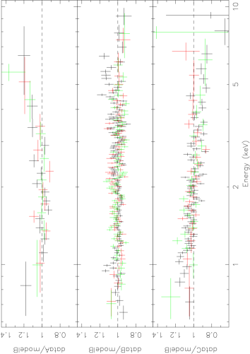
Independent of the adopted spectral model, it is clear from the best fit parameters reported in Table 2 that the spectrum changed between the different observations. This can also be seen from Fig.1, which shows the ratios between the spectra of the three observations and the best fit model of obs. B scaled only in overall normalization (the normalization factors are reported in the first line of Table 3). The spectrum of obs. C is significantly softer than the template spectrum, while that of obs. A is slightly harder, although, due to its poorer statistiscs, the fit is formally acceptable, as reported in Mereghetti et al. (2004).
For the sake of simplicity we tried to interpret the long term spectral variations using the model with less parameters, i.e the blackbody plus power law. In order to check whether the long term spectral variation could be ascribed to a change in only one or two of the four333the overall spectral shape, beside depending on NH, and kTBB, is a function of the relative normalization of the two components relevant parameters we fitted the spectra of obs. A and C keeping some of them fixed to the best fit values of obs. B. The results are summarized in Table 3, where one can see that the variations are described in an almost equivalent way by a change either in the blackbody temperature (which is slightly preferred for obs. A) or in the photon index (which gives a better fit to obs. C). If the photon index and temperature are kept fixed and only their relative normalization or the NH free to vary, a significant improvement in the value is obtained for obs. C but not for obs. A.
The possibility that one of the two spectral components remained constant (both in shape and normalization) throughout the three observations was also explored, with negative results. In fact, due to the flux variation between the two observations, fitting the spectrum of obs. A with the parameters of either the power law or the blackbody component fixed to those of obs.B gives 2 (even if the NH is left free to vary).
| Parameter(a) | A | C |
|---|---|---|
| Normalization factor | 0.4320.006 | 0.6580.004 |
| (d.o.f.) | 1.081 (261) | 1.341 (438) |
| NH (1022 cm-2) | 1.070.02 | 1.020.01 |
| Normalization factor | 0.429 | 0.632 |
| (d.o.f.) | 1.084 (260) | 1.112 (437) |
| RBB (km) | 0.840.03 | 0.960.02 |
| PL norm | 5.60.2 | 9.30.2 |
| (d.o.f.) | 1.084 (260) | 1.126 (437) |
| kTBB (keV) | 0.690.02 | 0.6020.008 |
| RBB (km) | 0.66 | 1.07 |
| PL norm | 6.00.2 | 9.00.2 |
| (d.o.f.) | 0.978 (259) | 1.073 (436) |
| 3.02 | 3.44 | |
| RBB (km) | 0.720.05 | 1.03 |
| PL norm | 5.6 | 9.3 |
| (d.o.f.) | 0.999 (259) | 1.040 (436) |
(a) The parameters not indicated in this Table have been
fixed to the best-fit values of obs.B given in the first part of Table 2
2.2 Phase resolved spectroscopy
After correcting the time of arrival of the source events to the Solar System barycenter, we carried out a standard timing analysis based on folding and phase fitting. The source period was clearly detected in all the observations, with the values given in Table 1. Note that the pulse period reported in Mereghetti et al. (2004) for obs. B is wrong. As a consequence, also the corresponding pulsed fraction (computed by fitting a sinusoid to the background subtracted light curve) is slightly larger than that previously reported. The folded light curves of the three observations are shown in Fig.2 (left panel). They are characterized by a single broad pulse of nearly sinusoidal shape and different levels of modulation in the three observations. We have computed the pulsed fraction by fitting the background subtracted pulse profiles with a constant plus a sinusoid. The pulsed fraction of each observation, defined as the ratio between the semi-amplitude of the sinusoid and the constant, is plotted as a function of the source flux in the right panel of Fig. 2.


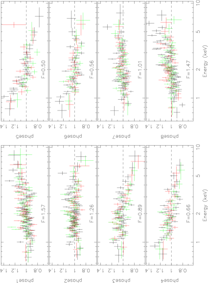
Phase resolved spectroscopy was performed first by dividing the data of obs. B in 8 phase intervals as indicated in Fig. 2. For each interval a spectrum was extracted and analyzed as described above for the phase averaged spectra. Again, to study the phase dependent variations, we adopted for simplicity the power law plus blackbody model. The spectra of the different intervals were first fitted keeping the parameters fixed at the best-fit values of the phase averaged spectrum, and allowing only the overall normalization factor to vary. The corresponding residuals and normalization factors, shown in Fig.3, clearly indicate that the spectrum is softer at pulse minimum and harder at maximum. To model these spectral variations, as a first step we allowed the normalizations of the two spectral components to vary independently. Then, also the blackbody temperature and power law photon index were left free to vary. The resulting best-fit values are plotted in Fig. 4. As it was found in the comparison of the phase averaged spectra, the spectral variations can be modelled equally well by a change in the blackbody or in the power law component. What is interesting is that, in any case, a change in the relative normalization of the two components is required.
The same kind of analysis applied to the other two observations444due to the small number of counts we used only three phase intervals for obs. A led to similar results. An example of this, for the case of fixed kTBB (fourth column of Fig. 4), is shown in Fig. 5.


2.3 Search for spectral features
We searched for spectral features in the EPIC spectra by first considering lines with a Gaussian profile and width narrower than the instrumental energy resolution (i.e. fixing =0) and then extending the search to broader lines (=100 eV). No spectral features were significantly detected. Since some deviations from the best fit models, which are most likely to be attributed to small calibration uncertainties were present in the residual, we adopted a conservative confidence level of 4 for the upper limits. These are given for the equivalent widths of either emission or absorption lines in Table 4.
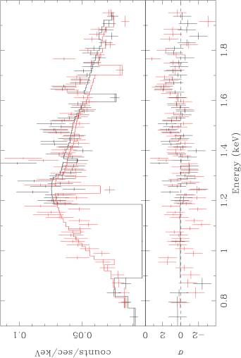
For obs. B, thanks to the long exposure time and high source flux, also the RGS instrument could be used for the spectral analysis. The RGS covers only the 0.35–2.5 keV range and has a smaller effective area than EPIC, but thanks to its higher energy resolution (5 eV at 1 keV compared to 80 eV of EPIC) it is very efficient in the search for narrow lines in the soft X–ray range. After a standard extraction of the RGS source and background spectra and the generation of the corresponding response files, the first order spectra555the higher order spectra do not have enough counts for a meaningful analysis. of the RGS1 and RGS2 instruments were rebinned in order to have at least 50 counts per bin. The spectra were then jointly fitted using the blackbody plus power law best fit parameters obtained with EPIC, leaving only a normalization factor for each RGS unit as free parameter. The values of these factors are 0.990.04 for RGS1 and 0.900.03 for RGS2, which are fully compatible with the known cross-calibration uncertainties. However, this fit is not formally acceptable (1.22/127) and some excess in the residuals is visible around 1.65 keV (see Fig.6). In fact, a significantly better fit (1.05/125) is obtained with the addition of a narrow emission line centered at 1.653 keV and with equivalent width 217 eV (90% confidence level). However the reality of this line is not confirmed by the higher statistics EPIC data: the 4 upper limit on the equivalent width of a narrow emission line at 1.653 keV in the EPIC spectrum of obs. B is 6.7 eV.
| Energy range | (eV) | Equivalent width |
|---|---|---|
| 1–2 keV | 0 | 10 eV |
| 100 | 20 eV | |
| 2–4 keV | 0 | 20 eV |
| 100 | 30 eV | |
| 4–5 keV | 0 | 30 eV |
| 100 | 55 eV | |
| 5–6 keV | 0 | 60 eV |
| 100 | 60 eV | |
| 6–7 keV | 0 | 90 eV |
| 100 | 150 eV | |
| 7–8 keV | 0 | 150 eV |
| 100 | 220 eV |
The search for spectral features was also extended to the EPIC phase resolved spectra (the smaller number of counts does not allow to use also the RGS for phase-resolved spectroscopy). No narrow features were detected in the 8 phase resolved EPIC spectra described in Section 2.2. The 4 upper limits for emission or absorption lines are typically a factor 2–5 higher than those reported in Table 4, depending on the pulse phase interval and energy range.
3 Discussion
The target of opportunity observation of July 2004 (obs. C) was motivated by the detection of one burst from the direction of 1E 1048.1–5937 with the RXTE satellite (Kaspi et al. 2004) and carried out nine days after this event. No bursts were seen during the XMM-Newton observation, nor any other sign indicating a particularly increased level of activity: the flux of 1E 1048.1–5937, 6.2 erg cm-2 s-1, was still 25% higher than the typical values observed before the 2001 outburst (see Fig.2 in Mereghetti et al. 2004 and Fig.1 in Gavriil & Kaspi 2004), but not as high as that measured in obs. B. We find statistically significant differences in the spectra of the three XMM-Newton observations, however such differences are not related in a monotonic way with the source luminosity: when the flux was at the highest level (obs. B) the spectral hardness was intermediate (see Fig.1).
A coherent pattern is instead present in the relation between flux and pulsed fraction: the latter decreases when the source brightens, as was first reported by Mereghetti et al. (2004) based only on two observations. This is confirmed by obs. C as shown in the right panel of Fig. 2, where, to avoid any cross calibration uncertainty, we directly compare the flux and pulsed fraction (PF) measured with the same detector in the three observations. The existence of an empirical anti-correlation between luminosity and pulsed fraction, independent on its theoretical explanation, must be taken into account in the interpretation of the RXTE results for this source. The luminosity and fluence obtained with this satellite, which can only measure the pulsed component of the flux, are clearly underestimated if the decrease in pulsed fraction during the outbursts is not taken into account. We estimate that total energy release of the flares peaking in November 2001 and June 2002 is at least the double of the value (2 and 20 ergs respectively) derived assuming a constant PF=.94 by Gavriil & Kaspi (2004).
Our results for the phase averaged spectroscopy are substantially in agreement with previous findings for this and other AXPs, except that the high statistics of obs. B allowed us to reject the fit with two blackbody components. We also explored spectral fits using a simple Comptonization model. The fit with the Comptonization model alone is not satisfactory. The addition, however, of a second, softer blackbody component, resulted in an acceptable fit, both for the phase-averaged, and for the phase-resolved spectra. Quite interestingly the estimate of the radiating area for the cooler component is in this case compatible with the entire star surface when the distance uncertainty is taken into account. Spectra at different phases can be fitted keeping this emitting area fixed at the value derived from the phase-averaged analysis and this results only in a modest variation of the cool blackbody temperature, , and a modulation of the hot blackbody emitting area. The smaller area associated with the hotter blackbody emission may be suggestive of a scenario in which a magnetically active region produces a hotter region contributing a substantial part of the luminosity. The accelerated high-energy particles, besides heating this region may upscatter the soft photons giving rise to the Comptonized spectrum.
The implementation of a detailed Comptonization model to fit the X–ray spectrum is beyond the scope of our analysis. Therefore, we have used the approximated model described in Section 2.1, which is based on a constant scattering cross-section. The scattering cross-section in a strongly magnetized medium is anisotropic and quite different for ordinary (O) and extraordinary (X) photons (e.g. Ventura 1979; Gonthier et al. 2000). In our case the typical incident photon energy is keV, well below the resonance at the electron cyclotron energy . In the low-frequency limit (), the cross section for ordinary photons is , where is the Thomson cross-section. Due to relativistic beaming, scattering occurs at an incident angle in the particle frame and therefore . For relativistic electrons of a given energy, the cross section for ordinary photons is therefore constant. The cross section for extraordinary photons, instead, peaks at , where . It means that, taking , it dominates over for . In this case the use of a constant cross-section is possible because we have checked numerically that its dependence on the photon spectrum has a negligible effect on the Comptonized spectrum.
The present model does not allow to univocally determine the properties of the Comptonizing medium, since the fitted parameter depends on both the scattering depth and the particle energy. However, with the presently derived values of the photon index, , once the Comptonizing particles are assumed to be relativistic electrons, the medium is optically thin and the optical depth is strongly anticorrelated to the particle energy (). For example, if , the magnetic depth is , to which corresponds a non-magnetic Thomson depth , while if , drops to , corresponding to a non-magnetic Thomson depth of .
Thanks to the high statistics of our observations we could set strong upper limits on the presence of spectral lines (in view of the EPIC results we do not consider the possible feature at 1.65 keV seen in the RGS as really present in the source). If interpreted in terms of magneto-dipolar braking, the spin-down rate measured with RXTE at the time of obs. B (Gavriil & Kaspi 2004) yields a dipolar field and at these field strenghts cyclotron, free-bound and free-free features are expected to lie in the observed energy band. On the other hand, present estimates of their detectability in the presence of superstrong magnetic fields still suffer from a number of approximations (Zane et al. 2002, Ho et al. 2003). Several effects, e.g. fast rotation and magnetic smearing, have been suggested to explain the absence of spectral lines in other sources (e.g. Braje & Romani 2002). Although the former does not apply to the present source, both cyclotron and atomic lines are sensitive to the local field strength and the contributions of surface elements with different values of may under certain conditions wash out spectral features. Ho & Lai (2004) also suggested that at super-strong field strengths ( G) vacuum polarization may efficiently suppress spectral lines, but current treatment of this QED effect is too crude to make a definite statement. The absence of lines may also suggest either that the magnetic field at the neutron star surface is larger than the large scale dipolar component (i.e. that ) or, alternatively, that the value inferred by the spin-down rate is overestimated (i.e. that ). As discussed by Thompson et al. (2002), this value must be regarded as an upper limit: a twisted magnetosphere may lead to a reduction up to an order of magnitude in the inferred polar value of the magnetic field, while the estimate of the spin down age is unaffected.
Phase resolved spectroscopy has now been carried out for most AXPs. The earlier observations obtained with the ASCA and BeppoSAX satellites gave some indications for phase-dependent spectral variations in 4U 0142614 (Israel et al. 1999), 1E 2259586 (Corbet et al. 1995, Parmar et al. 1998), 1E 1048.1–5937 (Oosterbroek et al. 1998), and a more significant evidence for 1RXS J1708–4009 (Israel et al. 2001). These indications were later confirmed by observations with higher statistics carried out with XMM-Newton (Tiengo et al. 2002, Woods et al. 2004, Göhler et al. 2004) and Chandra (Morii et al. 2003). In most of these studies the blackbody plus power-law was adopted and the spectral variations described as changes in one or more of the model parameters. The results reported here give strong evidence that the spectrum of 1E 1048.1–5937 is harder at pulse maximum. However the interpretation of this result is not straightforward since the values of the spectral parameters, e.g. blackbody temperature or photon index, are linked in a complex way to the overall spectral shape/hardness. As we have shown in the previous section, these variations can be modelled in different ways. For example (see Fig.4) if the photon index and blackbody temperature are fixed, the ratio is proportional to the total intensity. In turn, this means that the blackbody contribution at the pulse maximum is more important than that at the pulse minimum, i.e. that the blackbody component has a pulsed fraction larger than the power law. This is what is expected if the thermal component originates from the star surface and the non-thermal one from a more extended magnetosphere, and may lead to suggest that the observed spectral changes are simply due to the partial occultation of an the emitting regions as the star rotates, with the effect being more prominent for the surface emission than for the magnetosphere. On the other hand, better fits are obtained if also the photon index or the temperature are free to vary (third and fourth columns of Fig. 4). In this respect, probably the most interesting result is that we found impossible to reproduce the phase-dependent variations keeping one of the two components completely fixed (i.e. shape and normalization). This fact indicates a coupling between the two components, or alternatively, it strengthens a scenario in which the emission below 10 keV is dominated by a single physical mechanism with a spectrum more complex than a blackbody or a power-law.
4 Summary
The main conclusions derived from the analysis and comparison of the three XMM-Newton observations of 1E 1048.1–5937 reported here are the following:
-
•
long term flux variations of a factor 2 are accompanied by only minor, though statistically significant, changes in the source spectral properties
-
•
the pulsed fraction is anti-correlated with the source luminosity, decreasing from 90% to 55% in correspondence of a twofold increase in flux. This should be properly taken into account when the source energetics are inferred by measurements of the pulsed flux
-
•
spectral variations are clearly present as a function of the pulse phase, with the hardest spectrum at pulse maximum; their interpretation in terms of simple changes in two component models is not unique
-
•
there is no evidence for absorption and/or emission lines in the spectrum with equivalent width larger than 10-220 eV, depending on energy and width
-
•
the spectrum is consistent with a two component model consisting of a blackbody emission from an emitting area compatible with the whole neutron star surface and a hotter Comptonized blackbody, possibly coming from a relatively large region of the star surface heated by non-thermal magnetospheric particles also responsible for the scattering.
References
- (1) Braje T.M. & Romani R.W. 2002, ApJ 580, 1043
- (2) Corbet R.H.D, Smale A.P., Ozaki M. et al. 1995, ApJ 443, 786.
- (3) den Herder, J. W., et al. 2001, A&A, 365, L7
- (4) Duncan R.C. & Thompson C. 1992, ApJ 392, L9.
- (5) Gaensler et al. 2005, ApJ 620, L95
- (6) Gavriil F.P., Kaspi V.M. & Woods P.M. 2002, Nature 419, 142
- (7) Gavriil F.P. & Kaspi V.M. 2004, 609, L67
- (8) Göhler E., Wilms J. & Staubert R. 2004, astro-ph/0409764
- (9) Gonthier P.L., Harding A.K., Baring M.G. et al. 2000, ApJ, 540, 907
- (10) Halpern J.P. & Gotthelf E.V. 2004, ApJ in press, astro-ph/0409604
- Ho et al. (2003) Ho, W.C.G., et al., 2003, ApJ, 599, 1293
- Ho & Lai (2004) Ho, W.C.G., & Lai, 2004, ApJ, 607, 420
- (13) Israel G.L., et al. 1999, A&A 346, 929.
- (14) Israel G.L., et al. 2001, ApJ 560, L65
- (15) Kaspi, V. M. et al. 2003, ApJ 588, L93
- (16) Kaspi V., Gavriil F., Woods P. & Chakrabarty D. 2004, Astronomer’s Telegram, 298
- (17) Kirsch M. et al. 2004, preprint, astro-ph/0407257
- (18) Mereghetti S. & Stella L. 1995, ApJ 442, L17.
- (19) Mereghetti S., Chiarlone L., Israel G.L. & Stella L. 2002, in Neutron Stars, Pulsars and Supernova Remnants, eds. W.Becker, H.Lesch and J.Trümper, MPE-Report 278, 29.
- (20) Mereghetti, S., Tiengo, A., Stella L., Israel G.L., Rea, N., Zane, S., Oosterbroek, T. 2004, ApJ, 608, 427
- (21) Morii, M., Sato R., Kataoka J. & Kawai N. 2003, PASJ 55, L45
- (22) Oosterbroek T., Parmar A.N., Mereghetti S. & Israel G.L. 1998, A&A 334, 925.
- (23) Rybicki, G.B. & Lightman, A.P. 1979, Radiative Processes in Astrophysics (New York: Wiley)
- (24) Strüder L. et al. 2001, A&A 365, L18.
- (25) Thompson C. & Duncan R.C. 1996, ApJ 473, 322.
- Thompson et al. (2002) Thompson, C., Lyutikov, M., Kulkarni, S. R., 2002, ApJ, 574, 332
- (27) Tiengo A., Göhler E., Staubert R. & Mereghetti S. 2002, A&A 383, 182
- (28) Turner M.J.L. et al. 2001, A&A 365, L27.
- (29) van Paradijs J., Taam R.E. & van den Heuvel E.P.J. 1995, A&A 299, L41.
- (30) Ventura, J. 1979, Phys. Rev. D, 19, 19
- (31) Woods P.M. et al. 2004, ApJ 605, 378
- Zane et al. (2002) Zane, S., et al. 2002, MNRAS, 334, 345