Radiation in the process of the formation of voids

Abstract

This paper aims to investigate the influence of inhomogeneous radiation in void formation. Since the process of void formation is non–linear, a fully relativistic model, which simulates the evolution of voids from the moment of the last scattering until the present instant, is presented. It is found that in order to obtain a model of a void which evolves from $\delta_{0}=-10^{-5}$ at the last scattering moment to the present day $\delta=-0.94$, the existence of radiation must be taken into account. The ratio of radiation energy density to matter energy density in ${\rm CDM}$ models at the moment of last scattering is $1/5$. This paper proves that such a value of radiation energy density cannot be neglected and influences the first stages of void evolution. Namely, it is important to the process of structure formation and hence significantly influences the dynamics of the Universe in the first millions of years after the last scattering.

From the fact that the evolution of voids proceeds differently in various cosmological background models we use the process of void formation to put some limits on values of cosmological parameters. We find that the model with $\Omega_{mat}\sim 0.3$ fits the observational data best.

1 Introduction

At the end of the 1970s several galaxy redshift surveys started to operate. As a result the spatial distribution of a large sample of galaxies had been measured. It turned out that galaxies are distributed inhomogeneously and form structures like voids or clusters.

The most probable explanation of existence of such structures is that they evolved from small initial fluctuations. These fluctuations can be traced in the observations of the Cosmic Microwave Background (CMB).

While gravity is an attractive force, it is relatively easy to reproduce high density regions, for instance by setting the initial conditions so that collapse or shell crossings occur. This cannot be done in case of low density regions, such as voids, inside which the estimated value of the density contrast is less than $\delta=-0.94$ (which is less than $6\%$ of the mean background density) (Hoyle & Vogeley 2004). The description of evolution of voids from initial fluctuations consistent with observational constraints is very difficult. So far none of the attempts to solve this problem succeeded. Even N–body simulations predict that voids should be filled by dwarf galaxies which are not observed (Hoyle & Vogeley 2004).

In this paper we are going to present a scenario of void formation which is consistent with astronomical observations and leads to the formation of low density regions from very small initial fluctuations that existed at the moment of the last scattering.

As will be demonstrated, the evolution of voids is a non–linear process. That is why this approach is based on exact solutions of the Einstein equations.

The structure of this paper is as follows: in Sec. 2 the model to be used is presented. In Sec. 3 the initial conditions at the last scattering moment are presented. These data constrain values of parameters and functions used in the theoretical models. Since the influence of the gradient of pressure cannot be neglected, in Sec 4 an approximate and an analytical solution of a model with inhomogeneous distribution of radiation is presented. This model qualitatively shows that the gradient of pressure plays a significant role in the evolution of the Universe after the last scattering moment. In Sec. 6 results of and fully non–linear evolution of models with inhomogeneous radiation distribution are presented. In Sec. 6.3, constraints on the values of cosmological parameters are derived from the fact that the structure formation proceeds differently in various cosmological background models.

2 The spherically symmetric inhomogeneous space–time

A spherically symmetric metric in comoving and synchronous coordinates is of the form:

$${\rm d}s^{2}={\rm e}^{A(t,r)}c^{2}{\rm d}t^{2}-{\rm e}^{B(t,r)}{\rm d}r^{2}-R^{2}(t,r)\left({\rm d}\theta^{2}+\sin^{2}\theta{\rm d}\phi^{2}\right).$$ (1)

The Einstein field equations for the spherically symmetric perfect fluid distribution (in coordinate components) are:

$$G^{0}{}_{0} = {\rm e}^{-A}\left(\frac{\dot{R}^{2}}{R^{2}}+\frac{\dot{B}\dot{R}}{R}\right)-{\rm e}^{-B}\left(2\frac{R^{\prime\prime}}{R}\right.+$$ (2)

$$+ \left.\frac{R^{\prime 2}}{R^{2}}-\frac{B^{\prime}R^{\prime}}{R}\right)+\frac{1}{R^{2}}=\kappa\epsilon+\Lambda,$$

$$G^{1}{}_{0} = {\rm e}^{-B}\left(2\frac{\dot{R}^{\prime}}{R}-\frac{\dot{B}R^{\prime}}{R}-\frac{A^{\prime}\dot{R}}{R}\right)=0,$$ (3)

$$G^{1}{}_{1} = {\rm e}^{-A}\left(2\frac{\ddot{R}}{R}+\frac{\dot{R}^{2}}{R^{2}}-\frac{\dot{A}\dot{R}}{R}\right)+$$ (4)

$$- {\rm e}^{-B}\left(\frac{R^{\prime 2}}{R^{2}}+\frac{A^{\prime}R^{\prime}}{R}\right)+\frac{1}{R^{2}}=-\kappa p+\Lambda,$$

$$G^{2}{}_{2} = G^{3}{}_{3}=\frac{1}{4}{\rm e}^{-A}\left(4\frac{\ddot{R}}{R}-2\frac{\dot{A}\dot{R}}{R}+2\frac{\dot{B}\dot{R}}{R}+\right.$$ (5)

$$+ \left.2\ddot{B}+\dot{B}^{2}-\dot{A}\dot{B}\right)-\frac{1}{4}{\rm e}^{-B}\left(4\frac{R^{\prime\prime}}{R}+2\frac{A^{\prime}R^{\prime}}{R}+\right.$$

$$- \left.2\frac{B^{\prime}R^{\prime}}{R}+2A^{\prime\prime}+A^{\prime 2}-A^{\prime}B^{\prime}\right)=-\kappa p+\Lambda,$$

where $\epsilon$ is the energy density and $p$ is the pressure. $\dot{}$ stands for $\partial_{t}$ and ^′ stands for $\partial_{r}$. For a mixture of matter and radiation, we have:

$$\epsilon = \epsilon_{mat}+\epsilon_{rad},$$ (6)

$$p = \frac{1}{3}\epsilon_{rad}.$$ (7)

The Einstein equations can be reduced to (Lemaitre 1933):

$$\kappa R^{2}R^{\prime}\epsilon=2M^{\prime},$$ (8)

$$\kappa R^{2}\dot{R}p=-2\dot{M},$$ (9)

where $M$ is defined by:

$$2M(r,t) = R(r,t)+R(r,t){\rm e}^{-A(t,r)}{\dot{R}}^{2}(r,t)+$$ (10)

$$- {\rm e}^{-B(t,r)}{R^{\prime}}^{2}(r,t)R(r,t)-\frac{1}{3}\Lambda R^{3}(r,t).$$

In a Newtonian limit $Mc^{2}/G$ is equal to the mass inside the shell of radial coordinate $r$. However, it is not an integrated rest mass but active gravitational mass that generates a gravitational field. As it can be seen in eq. (10) the mass is not constant in time and in the expanding universe it decreases, as seen from (9).

From the equations of motion ${T^{\alpha\beta}}_{;\beta}=0$ we obtain:

$$T^{0\alpha}{}_{;\alpha}=0 \Rightarrow \dot{B}+4\frac{\dot{R}}{R}=-\frac{2\dot{\epsilon}}{\epsilon+p},$$ (11)

$$T^{1\alpha}{}_{;\alpha}=0 \Rightarrow A^{\prime}=-\frac{2p^{\prime}}{\epsilon+p},$$ (12)

$$T^{2\alpha}{}_{;\alpha}=0 \Rightarrow \frac{\partial p}{\partial\theta},=0,$$ (13)

$$T^{3\alpha}{}_{;\alpha}=0 \Rightarrow \frac{\partial p}{\partial\phi}=0.$$ (14)

Equations (13) and (14) reproduce the well known fact that the perfect fluid energy–momentum tensor inherits the symmetries of the metric of the space–time.

The $B$ function can be derived from eq. (3):

$$B(r,t)=B(r,t_{0})+\ln R^{\prime 2}-\int\limits_{t_{0}}^{t}{\rm d\tilde{t}}\frac{A^{\prime}\dot{R}}{R^{\prime}}.$$ (15)

Using eq. (12) we obtain:

$${\rm e}^{B(r,t)}=\frac{R^{\prime 2}(r,t)}{1+2E(r)}\times$$

$$\exp\left(\int\limits_{t_{0}}^{t}{\rm d\tilde{t}}\frac{2\dot{R}(r,\tilde{t})}{\left[\epsilon(r,\tilde{t})+p(r,\tilde{t})\right]R^{\prime}(r,\tilde{t})}p^{\prime}(r,\tilde{t})\right),$$ (16)

where $E(r)$ is an arbitrary function.

2.1 The Lemaître–Tolman model

If the dust equation of state is considered, the above model becomes the Lemaître-Tolman model. As follows from eq. (12) and eq. (16), if $p^{\prime}=0$ then:

$${\rm e}^{A} = 1,$$ (17)

$${\rm e}^{B} = \frac{R^{\prime}}{1+2E}.$$ (18)

Then the metric (1) becomes:

$${\rm d}s^{2}=c^{2}{\rm d}t^{2}-\frac{R^{\prime 2}(r,t)}{1+2E(r)}\ {\rm d}r^{2}-R^{2}(t,r){\rm d}\Omega^{2},$$ (19)

where ${\rm d}\Omega^{2}={\rm d}\theta^{2}+\sin^{2}\theta{\rm d}\phi^{2}$. Because of the signature $(+,-,-,-)$, the $E(r)$ function must obey $E(r)\geq-\frac{1}{2}.$

The Einstein equations reduce to the following two:

$$\kappa\rho c^{2}=\frac{2M^{\prime}}{R^{2}R^{\prime}},$$ (20)

$$\frac{1}{c^{2}}\dot{R}^{2}=2E+\frac{2M(r)}{R}+\frac{1}{3}\Lambda R^{2},$$ (21)

where $M(r)$ is another arbitrary function and $\kappa=\frac{8\pi G}{c^{4}}$.

When $R^{\prime}=0$ and $M^{\prime}\neq 0$, the density becomes infinite. This happens at shell crossings. This is an additional singularity to the Big Bang that occurs at $R=0,M^{\prime}\neq 0$. Shell crossing can be avoided by setting the initial conditions appropriately.

Equation (21) can be solved by simple integration:

$$\int\limits_{0}^{R}\frac{d\tilde{R}}{\sqrt{2E+\frac{2M}{\tilde{R}}+\frac{1}{3}\Lambda\tilde{R}^{2}}}=c\left(t-t_{B}(r)\right),$$ (22)

where $t_{B}$ appears as an integration constant, and is an arbitrary function of $r$. This means that the Big Bang is not a single event as in the Friedmann models, but occurs at different times at different distances from the origin.

Thus, the evolution of a Lemaître-Tolman model is determined by three arbitrary functions: $E(r)$, $M(r)$ and $t_{B}(r)$. The metric and all the formulae are covariant under arbitrary coordinate transformations of the form $r=f(r^{\prime})$. Using such a transformation, one function can be given a desired form. Therefore the physical initial data for the evolution of the Lemaître-Tolman model consist of two arbitrary functions.

2.2 The Friedmann limit

Assuming homogeneity, the above model becoms the Friedmann model.

In the class of coordinates used here, one can choose the radial coordinate as:

$$R(r,t)=ra(t),$$ (23)

Then:

$$M(r,t)=M_{0}r^{3},$$ (25)

$$2E(r)=-kr^{2}.$$ (26)

$${\rm e}^{A(r,t)}\to 1,$$ (27)

$${\rm e}^{B(r,t)}\to\frac{a^{2}}{1-kr^{2}},$$ (28)

$$\kappa\epsilon=\frac{6M}{R^{3}}$$ (29)

where $a$ is the scale factor and $k$ is the curvature index of the Friedmann models. Then the metric becomes:

$${\rm d}s^{2}=c^{2}{\rm d}t^{2}-a(t)^{2}\left(\frac{{\rm d}r^{2}}{1-kr^{2}}-r^{2}\left({\rm d}\theta^{2}+\sin^{2}\theta{\rm d}\phi^{2}\right)\right).$$ (30)

The condition $T^{\alpha\beta};_{\beta}=0$, reduces to:

$$\dot{\rho}+3\frac{\dot{a}}{a}\left(\rho+\frac{p}{c^{2}}\right)=0.$$ (31)

Assuming the dust equation of state, eqs. (4), and (10) become the Friedmann equations:

$$2\frac{\ddot{a}}{a}=-\frac{1}{3}\kappa c^{4}\rho+\frac{2}{3}\Lambda c^{2},$$ (32)

$$\dot{a}^{2}=-kc^{2}+\frac{1}{3}\kappa c^{4}\rho a^{2}+\frac{1}{3}\Lambda c^{2}a^{2}$$ (33)

The Friedmann limit is an essential element in our approach. As mentioned above, our model of void formation describes a single void in an expanding Universe. Far away from the origin, the density and velocity distributions tend to the values that they would have in a Friedmann model. Consequently the values of the time instants (i.e. initial — $t_{0}$ and final — $t_{f}$ instants) and values of the density and velocity fluctuations are calculated with respect to this homogeneous background.

3 Constraints on the initial conditions

Voids are vast regions in which hardly any galaxies are observed. An average radius of a void is $12~{}h^{-1}$ Mpc and the density contrast inside is $-0.94$ (Hoyle & Vogeley 2004). Such structures must have evolved from small initial fluctuations that existed at the last scattering instant. In this section the estimation of the initial conditions is presented.

3.1 Observational constraints

The observations of the CMB provide us with the redshift of the surface of the last scattering. Once the redshift is known, density of matter, density of radiation, temperature and pressure can be estimated. The measured value of the temperature fluctuations, $\Delta T\approx 10^{-5}$ can be converted into density and velocity fluctuations of a baryonic matter at that time. The estimated amplitude of the initial fluctuations, inside the voids, are (Bolejko, Krasiński & Hellaby 2005):

• density fluctuations — $\Delta\rho/\rho=\delta=-6\cdot 10^{-5}$

• velocity fluctuations — $\Delta V/V_{b}=\nu=2\cdot 10^{-4}$

The observed redshift of the CMB is $z\approx 1090$. At that redshift the amplitude of pressure of matter can be estimated from the perfect gas equation of state:

$$\frac{p}{\rho c^{2}}=\frac{k_{B}T}{\mu m_{H}c^{2}}\approx 10^{-10}.$$ (34)

This estimation shows that the pressure of matter after the last scattering moment is negligible in the evolution of the Universe.

The contribution of radiation to the energy density cannot be neglected and the ratio of radiation energy density to matter energy density at the last scattering moment is:

$$\frac{\epsilon_{rad}}{\epsilon_{mat}}=\frac{aT^{4}}{\rho c^{2}}=\frac{\Omega_{\gamma}}{\Omega_{m}}(1+z),$$ (35)

where $a=4\frac{\sigma}{c}$ and $\sigma$ is Stefan–Boltzmann constant; $\Omega_{\gamma}=\frac{aT_{CMB}^{4}}{\rho_{cr}}$ and $T_{CMB}$ is the current temperature of the CMB background; $\rho_{cr}$ is critical density and is equal to $(3H_{o})/(8\pi G)$.

At the moment of last scattering, for $\Omega_{mat}=0.3$ this is:

$$\frac{\epsilon_{rad}}{\epsilon_{mat}}\approx 0.2.$$ (36)

As can be seen, this ratio decreases for low redshifts. However, at the early stage of the evolution after the last scattering moment the radiation should have an influence on the evolution of the Universe. This issue will be considered futher.

3.2 Initial fluctuations in the linear approach

Although the present–day density contrast inside voids is large ($\delta\approx-0.9$) and it is unlikely that the linear approximation might handle it appropriately, the following calculations are presented to provide a comparison. Let us assume that the Universe is homogeneous with only small perturbations of the form:

$$a = a_{b}(1+\alpha(r,t))$$ (37)

$$\rho = \rho_{b}(1+\delta(r,t)).$$ (38)

Inserting these perturbations into eq. (32) and using eq. (31) we obtain:

$$\ddot{\delta}+2\frac{\dot{a}_{b}}{a_{b}}\dot{\delta}-\frac{1}{2}\kappa c^{2}\rho_{b}\delta=0$$ (39)

In the simplest case, i.e. the Einstein–de Sitter model, this equation reduces to:

$$\ddot{\delta}+\frac{4}{3ct}\dot{\delta}-\frac{2}{3c^{2}t^{2}}\delta=0,$$ (40)

and has the analytical solution:

$$\delta=C_{1}\tau^{2/3}+C_{2}\tau^{-1},$$ (41)

where $\tau$ is dimensionless time, i.e. $\tau=t/t_{0}$.

As can be seen, the first factor describes the growing mode, while the second factor describes the decaying mode. Assuming that only the growing mode exists, we obtain:

$$\delta=\delta_{0}\tau^{2/3},$$ (42)

where $\delta_{0}$ is the initial density contrast.

Assuming that the present-day density contrast of voids is $\delta=-0.9$, for the Einstein–de Sitter model, $\tau=t_{U}/t_{LS}\approx 3.5\times 10^{4}$ (where $t_{U}$ is the age of the Universe and $t_{LS}$ is the last scattering instant), we obtain:

$$\delta_{0}\approx 8\times 10^{-4}.$$ (43)

However, due to the very large present-day value of the density contrast inside voids the linear approximation is inadequate. Moreover, the solutions of the formula (39) have neither upper, nor lower, limit. The mathematical structure of this equation allows the solution to be of any value, even of large negative value. However from the physical point of view it is impossible to have a density contrast lower than $\delta_{lim}=-1$. Unlike the linear approximation, the real density contrast inside the voids should asymptotically approach $-1$. Therefore, this relation is invalid in investigation of void formation and an fully non–linear solution must be considered.

3.3 Initial fluctuations in the Lemaître–Tolman model

Evolution of voids in the Lemaître–Tolman model was considered in Bolejko, Krasiński and Hellaby (2005). In that paper the evolution of a void from small initial velocity and density fluctuations is investigated. The results imply that the existence of present–day voids requires the amplitude of the initial density and velocity fluctuations to be of $\delta\sim\nu\approx 5\times 10^{-3}$.

These results are by one order of magnitude larger than the results obtained in the linear approach. Fig. 1 presents the evolution of the density contrast in the linear approximation and in the Lemaître–Tolman model. Both models are of the same initial conditions, $\delta_{0}=3\times 10^{-3}$. As expected, the density contrast decreases more slowly in the non–linear model than in the linear approach. The difference between the results greater than $10\%$ starts at $\tau\approx 500$, which corresponds to a redshift of $z\approx 15$. For redshifts larger than $z=15$ the linear approach reproduces the results with error larger than $10\%$, and for $\tau\approx 7000$ ($z\approx 2.25$) the density contrast is below $-1$ which is unphysical.

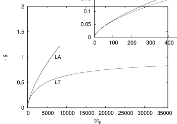
Figure 1: The evolution of the density contrast in the linear approach and in the Lemaître–Tolman model. Both models are of the same initial fluctuations, $\delta_{0}=3\times 10^{-3}$. For $\tau>7000$ the linear approach predicts a density contrast lower than $-1$, which is not physical.

Such a disproportion between the theoretical prediction ($\delta_{0}\sim 10^{-3}$) and the observational measurements ($\delta_{0}\sim 10^{-5}$) can be interpreted in two ways. The first alternative is that the dark matter is made of some weakly interacting massive particles, which at the moment of the last scattering could have the amplitude of fluctuation of $10^{-3}$. The second interpretation is that the matter fluctuations at the last scattering moment were of $10^{-5}$ and to obtain results consistent with observations some other effects must be taken into account. As was presented in Sec. 3.1, radiation is not negligible and might influence the evolution of voids. Although it seems rather unlikely that introduction of a small amount of radiation (temperature fluctuations at the last scattering moment were of $\sim 10^{-5}$) could have a significant impact on void evolution, it will be shown below that in reality the radiation component plays an important dynamical role. It will be also shown that the linear approximation is inadequate here, and that the influence of radiation must be considered in the non–linear formalism of relativity. In the next section an approximate model with inhomogeneous distribution of radiation is presented.

4 Approximate solution

As long as all fluctuations are very small the linear approach should be able to reproduce the proper results. Let us consider an approximate solution in the linear regime.

In comparison with Sec. 3.2 let us consider the $\Omega_{mat}=1,~{}\Omega_{\Lambda}=0$ model with a small perturbation of radiation. Despite the existence of radiation let us assume that unperturbed quantities are the same as in the Einstein–de Sitter model:

$$k=0\rightarrow E(r)=0$$ (44)

$$R_{0}=ra_{b}=ra_{0}\left(\frac{t}{t_{0}}\right)^{2/3}$$ (45)

$$\frac{\dot{a}_{b}}{a_{b}}=\frac{2}{3t}$$ (46)

$$\rho=\rho_{b}=\widetilde{\rho_{0}}\left(\frac{t}{t_{0}}\right)^{-2}=\frac{1}{6\pi Gt^{2}}$$ (47)

Futhermore, as only the pressure fluctuations are of our interest let us assume that initial velocity and density fluctuations are equal to zero. Radiation is as follows:

$$\xi=\xi_{b}(1+\gamma)$$ (48)

$$\xi_{b}=\frac{1}{20}\widetilde{\rho_{0}}c^{2}\left(\frac{t}{t_{0}}\right)^{-8/3}$$ (49)

$$p=\frac{1}{3}\xi=\frac{1}{3}\xi_{b}(1+\gamma)=\frac{1}{3}\xi_{b}\left(1+\gamma_{0}\exp(-r^{2}/L^{2})\right),$$ (50)

where $L^{2}$ is the size of the perturbed region of radius $5$ kpc at the last scattering moment. $\gamma_{0}=8\cdot 10^{-5}$ and is the amplitude of radiation fluctuation. Based on eq. (35) for $\Omega_{mat}=1$ the ratio of radiation energy density to matter energy density is $1/20$ and that is why in eq. (49) this value appears.

The density contrast is:

$$\delta=\frac{\rho-\rho_{0}}{\rho_{0}}$$ (51)

In the Friedmann limit, eq. (29):

$$\kappa c^{2}\rho\rightarrow\frac{6M}{R^{3}},~{}~{}~{}~{}~{}~{}~{}~{}~{}\kappa c^{2}\rho_{0}=\frac{6M_{0}}{R_{0}^{3}}=3\left(\frac{\dot{R}_{0}}{R_{0}}\right)^{2}=\frac{\kappa c^{2}}{6\pi Gt^{2}}$$ (52)

From eq. (10) and the assumption that there are no density and velocity fluctuations:

$$\frac{2M}{R^{3}}={\rm e}^{-A}\left(\frac{\dot{R}_{0}}{R_{0}}\right)^{2}-{\rm e}^{-B(t,r)}\left(\frac{R_{0}^{\prime}}{R_{0}}\right)^{2}+\frac{1}{R_{0}^{2}}-\frac{1}{3}\Lambda$$ (53)

In the following, we assume that $\Lambda=0$ (at the last scattering and a few billion years after the $\Lambda$ is negligible), and $A=0$.

Under these assumptions:

$$\delta=-\frac{3\frac{{\rm e}^{-B}{R^{\prime 2}}-1}{R^{2}}}{\frac{\kappa c^{2}}{6\pi Gt^{2}}}$$ (54)

Let us focus on the numerator first. Using eq. (16):

$$\frac{{\rm e}^{-B(t,r)}{R^{\prime}}^{2}(r,t)-1}{R^{2}}=\frac{(1+2E(r))}{R^{2}}\times$$

$$\exp\left(-\int\limits_{t_{0}}^{t}{\rm d\tilde{t}}\frac{2\dot{R}(r,\tilde{t})}{\left[\epsilon(r,\tilde{t})+p(r,\tilde{t})\right]R^{\prime}(r,\tilde{t})}p^{\prime}(r,\tilde{t})\right)+$$

$$-\frac{1}{R^{2}}:=\frac{\mathcal{I}}{R^{2}}$$ (55)

Applying the assumption stated at the beginning of this section and assuming that:

$$\frac{p_{0}}{\rho_{0}c^{2}+(4/3)p_{0}}\approx\frac{p_{0}}{\rho_{0}c^{2}},$$ (56)

$$\mathcal{I}=\exp\left(-\int\limits_{t_{0}}^{t}{\rm d\tilde{t}}\frac{2\dot{R}(r,\tilde{t})p^{\prime}(r,\tilde{t})}{\left[\epsilon(r,\tilde{t})+p(r,\tilde{t})\right]R^{\prime}(r,\tilde{t})}\right)-1$$ (57)

Applying series expansion to the $\exp$:

$$\mathcal{I}=\frac{1}{60}2\gamma_{0}\frac{2r}{L^{2}}\exp(-\frac{r^{2}}{L^{2}})\int\limits_{t_{0}}^{t}{\rm d\tilde{t}}\frac{\rho_{0}\tau^{-8/3}}{\left[\rho_{0}\tau^{-2}\right]}\frac{\dot{R}}{R^{\prime}}$$ (58)

$$\mathcal{I}=\frac{1}{60}2r\gamma_{0}\frac{2r}{L^{2}}\exp(-\frac{r^{2}}{L^{2}})\int\limits_{1}^{\tau}{\rm d\tau^{\prime}}\frac{\rho_{0}\tau^{-8/3}}{\left[\rho_{0}\tau^{-2}\right]}\frac{2}{3\tau}$$ (59)

Close to the origin, $r\approx 0$:

$$\mathcal{I}=\frac{8}{180}r^{2}\frac{\gamma_{0}}{L^{2}}\int\limits_{1}^{\tau}{\rm d\tau^{\prime}}\tau^{-5/3}$$ (60)

$$\mathcal{I}=\frac{1}{15}r^{2}\frac{\gamma_{0}}{L^{2}}(1-\tau^{-2/3})$$ (61)

As can be seen, $\mathcal{I}$ has the maximal value, :

$$I_{max}=\frac{1}{15}r^{2}\frac{\gamma_{0}}{L^{2}}$$ (62)

Inserting the above to eq. (54):

$$\delta=-3\frac{\frac{\mathcal{I}}{R^{2}}}{\frac{\kappa c^{2}}{6\pi Gt^{2}}}=-\frac{3}{20}\frac{c^{2}t_{0}^{2}}{L^{2}a_{0}^{2}}\tau^{2/3}$$ (63)

To calculate the value of the coefficient, we assume that at $t_{0}=t_{LS}$, $a_{0}=1$. Then:

$$\delta=-3\times 10^{-3}\tau^{2/3}$$ (64)

Comparing this result with eq. (42) it is easy to see that introducing only pure radiation fluctuation, the results are the same as the results obtained in the linear approach without any radiation component. The corresponding initial density fluctuation in the linear approach would be:

$$\delta_{0}=-3\times 10^{-3}$$ (65)

This proves that radiation is of great importance in voids evolution. However to be able to obtain precise predictions, more accurate calculations are needed. The evolution of voids within an non–linear model is presented in next section.

5 The algorithm

The computer algorithm used to calculate the evolution of a void was written in Fortran and consisted of the following steps. Numerical methods are from Press et al. (1986) and Pang (1997).

5.1 The initial data

5.1.1 Time instants

As follows from Sec. 2 to specify the model, one needs to know three functions. In this case these function are: density, velocity and radiation distribution functions, and are presented in subsections below. Because it is required that at large distace from the origin the model of a void becomes an homogeneous Friedman model, these functions are presented in form of given fluctuations imposed on the homogeneous background. All background values are calculated for the time instants obtained from the follwing formula (Peebles 1993):

$$t(z)=\frac{1}{H_{o}}\int\limits_{z}^{\infty}\frac{d\tilde{z}}{(1+\tilde{z})\sqrt{\mathcal{D}(\tilde{z})}},$$ (66)

where:

$$\mathcal{D}(z)=\Omega_{\gamma}(1+z)^{4}+\Omega_{mat}(1+z)^{3}+\Omega_{K}(1+z)^{2}+\Omega_{\Lambda},$$ (67)

$H_{o}$ is the present Hubble constant, $\Omega_{K}=1-\Omega_{\gamma}-\Omega_{mat}-\Omega_{\Lambda}$. The initial instant ($t_{0}$) is set to be at the last scattering moment, which took place when $z\approx 1089$ (Bennett et al. 2003) and the final instant ($t_{f}$) when $z=0$.

5.1.2 The initial density perturbations

The radial coordinate was defined as the areal radius at the moment of last scattering, measured in kiloparsecs:

$$r=\ell=R_{0}/d=R(r,t_{0})/d$$

where $d=1$ kpc.

The initial density fluctuations, imposed on the homogeneous background, were defined by functions of the radius $\ell$, as listed in Tables 1 and 2, and the actual density fluctuations followed from:

$$\rho_{0}(\ell)=\rho_{b{}0}\cdot\delta(\ell),$$ (68)

where $\rho_{b{}0}$ is the density of the homogeneous background and at the initial instant, and can be expressed as:

$$\rho_{b{}0}=\Omega_{mat}\rho_{cr}(1+z)^{3}.$$ (69)

The mass inside the shell of radius $R(r,t_{0})$ at the initial instant, measured in kiloparsecs, was calculated by integrating eq. (8):

$$M(\ell,t_{0})-M(0,t_{0})=\left.\frac{\kappa c^{2}}{2}\int\limits_{\ell_{min}}^{\ell}\rho_{i}(\ell^{\prime})\ell^{\prime 2}d\ell^{\prime}\right|_{t=t_{1}}.$$ (70)

Since the density distribution has no singularities or zeros over extended regions, it was assumed that $\ell_{min}=0$ and $M=0$ at $\ell=0$.

5.1.3 The initial velocity perturbations

The initial velocity fluctuations, imposed on the homogeneous background, were defined by functions of the radius $\ell$, as listed in Tables 1 and 2, and the actual velocity fluctuations followed from:

$$U(\ell)=U_{b{}0}\cdot\nu(\ell),$$ (71)

where $U_{b{}0}$ is the velocity of the homogeneous background at the initial instant, and can be expressed, from eq. (23), as:

$$U_{b}=\frac{1}{c}\dot{R}=\frac{1}{c}r\dot{a}.$$ (72)

In the FLRW models the time derivative of the scale factor is given by the formula (Peebles 1993):

$$\dot{a}=aH_{o}\sqrt{\mathcal{D}}.$$ (73)

Consequently:

$$U=(1+\nu)\frac{1}{c}RH_{o}\sqrt{\mathcal{D}}.$$ (74)

In the Lemaître–Tolman models the proper–time derivative of the areal radius $R$ ($U$) is just equal to $\frac{1}{c}\dot{R}$, in our case, in consequence of the metric (1):

$$U=\frac{1}{c}{\rm e}^{-A/2}\dot{R}.$$ (75)

5.1.4 The radiation perturbations

In FLRW models the equations of motion reduce to (Plebański & Krasiński 2005):

$$\partial_{t}(\epsilon a^{3})+3a^{2}\dot{a}p=0$$ (76)

For matter and radiation background (eqs. (6) and (7)) this equation becomes (to simplify the notation, we denote $\epsilon_{rad}=\mathcal{E}$ and $\epsilon_{mat}=\rho$):

$$(\dot{\mathcal{E}}+\dot{\rho})a^{3}+3(\mathcal{E}+\rho)a^{2}\dot{a}+a^{2}\dot{a}\mathcal{E}=0.$$ (77)

After the last scattering moment the radiation has not been interacting with matter, so we can assume that the evolution of matter is the same as in the Universe without radiation, i.e.:

$$\rho=\rho_{o}\left(\frac{a_{o}}{a}\right)^{3}.$$

Then from (77):

$$\mathcal{E}=\mathcal{E}_{o}\left(\frac{a_{o}}{a}\right)^{4}.$$

In the inhomogeneous Universe the radiation can be written in the following form:

$$\epsilon_{rad}(r,t)=\mathcal{E}(t_{f})(1+z)^{4}\zeta(r,t),$$ (78)

where $\zeta(r,t)$ is the function which describes the distribution and the evolution of radiation.

According to the current paradigm, after the last scattering moment the distribution of radiation has been ”frozen”. Consequently the only change in the radiation distribution is in the amplitude, which decreases with time, as the Universe expands:

$$\zeta(r,t)=\phi(t)\gamma(r)$$ (79)

The crucial problem is to find the form of the $\phi$ function. Luckily, the fluctuations of the radiation are very small, of amplitude $\sim 10^{-5}$, therefore, we can assume that the time–dependent amplitude of the radiation is the same as in the homogeneous background, so:

$$\phi=1.$$ (80)

However, this assumption may have to be modified in the future if observational data on the distribution of radiation become more detailed.

Recapitulating:

$$\epsilon_{rad}(\ell,z(t))=4\frac{\sigma}{c}T^{4}_{CMB}(1+z)^{4}\cdot\gamma(\ell)),$$ (81)

where $\sigma$ is the Stefan-Boltzmann constant, $c$ is the speed of light, $T_{CMB}$ is the current measured temperature of the CMB and $\gamma$ describes the initial perturbation of radiation, as listed in Tables 1 and 2.

Solving (66) with the bisection method the value of $z$ for some instant $t$ can be found. Substituting this value to (81) the value of energy density of radiation for this instant can be calculated.

5.2 Computing the evolution

The algorithm of the evolution consisted of the following steps:

1. From eqs. (75) and (12) the value of $\dot{R}$ and from (9) the value of $\dot{M}$ can be calculated. Then using the predictor–corrector method the value of $R(r,t+\tau)$ and $M(r,t+\tau)$ in the time step of $\tau$ can be found. We futher denoted them (as all the quantities found in this time step) by the subscript _τ.

2. Once $R_{\tau}$ and $M_{\tau}$ are known, we can derive $\epsilon_{\tau}$ from (8).

3. Then from (7) and (81) we derive $p_{\tau}$.

4. From $\epsilon_{\tau}$ and $p_{\tau}$ we can calculate $A_{\tau}$ by integrating eq. (12).

5. $U_{\tau}$ can be calculated as follows:

   From eq. (15) and (10) we obtain:

   $$U^{2}(r,t)=\frac{2M(r,t)}{R(r,t)}+\frac{1}{3}\Lambda R^{2}(r,t)-1$$

   $$+{\rm e}^{-B(r,t_{0})}{\rm e}^{\int_{t_{0}}^{t}{\rm d\tilde{t}}\left(A^{\prime}(r,\tilde{t}){\rm e}^{A(r,\tilde{t})/2}U(r,\tilde{t})\right)/R^{\prime}(r,\tilde{t})}.$$ (82)

   By solving this equation by the bisection method, for the time $t=t_{0}+\tau$ we can calculate $U_{\tau}$.

6. Once $U_{\tau}$ and $A_{\tau}$ are known, $\dot{R}(r,t)$ and futher $\dot{M}(r,t)$ can be calculated.

7. We repeat steps 1–6 until $t=t_{f}$.

6 Results

The measurements of density contrast inside voids are based on the observations of galaxies inside them (Hoyle & Vogeley 2004). However, because in central regions no galaxies are observed, the real density distribution inside the voids is unknown. Assuming that luminous matter is a good tracer of dark matter distribution and extrapolating the value of the density contrast measured on the edges of voids (where galaxies are observed) into the central regions of voids, we can conclude that the density inside the voids is below the value of $0.06\rho_{b}$. This value will be called the limiting value. It is expected that the model will predict a present–day density inside the voids below this limiting value.

While the problem of choice of the cosmological model is open and the efforts to determine the values of $\Omega_{mat}$ and $\Omega_{\Lambda}$ still continue, in this section (except subsection 6.3) we focused only on the cosmological model which is the most popular in the cosmological comunity, that is $\Lambda{\rm CDM}$ model.

Figure 2 shows the shape of the initial perturbations. The explicit forms of these perturbations are presented in Tables 1 and 2. The results are presented in Fig 3. In four out of seven model voids were formed. As can be seen, models with inhomogeneous distribution of radiation have no problems with reproducing regions of density below the limiting value.

To compare our results with the observational data, Fig. 4 presents the average density contrast inside the voids as a function of a relative distance from the origin. The average density contrast was calculated as follows:

$$\delta=\frac{<\rho>}{\overline{\rho}}-1,$$ (83)

where $\overline{\rho}$ is the present background density and $<\rho>$:

$$<\rho>=\frac{3Mc^{2}}{4\pi GR^{3}}.$$ (84)

Curve 1 presents the results of run 1, as listed in Table 1. Curves NGP and SGP corespond to density contrasts of voids in the 2dFGRS data estimated by Hoyle & Vogeley. Although the profiles match at the center they do not fit accurately at the edges of voids. In our model the density contrast tends to increase faster than the observed one which could be caused by too strong assumptions about the evolution of radiation ((79) and (80)) and would suggest that the distribution of radiation did evolve after the last scattering moment. There is another possibility that could explain the difference between these two profiles. The density contrast estmated by Hoyle & Vogeley is based on observations of galaxies. It is possible that the existence of dark matter in walls would make the real density higher than that estimated from counting of galaxies.

6.1 Initial perturbations

Introducing radiation into the calculation we need to know the relation between matter and radiation perturbations. In linear theory there are three concepts of these relations:

1. adiabatic perturbations, where $\gamma=\frac{4}{3}\delta$,

2. isocurvature perturbations, where $\gamma=\frac{4}{3}(\delta-\delta_{o})$; ($\delta_{o}$ is some initial value of $\delta$)

3. isothermal perturbation, where $\gamma=0$.

It should be stressed that in realistic conditions there are no pure adiabatic or isocurvature, or isothermal perturbations and the relations between density and radiation perturbations are more complicated. However, it is instructive to know what kind of relation is more suitable for the process of void formation.

Table 1: The initial Density Perturbations used in the runs.

Run	Profile	Description
1	$\delta_{-}=1-\mathcal{F}$	Isocurvature–like perturbation.
	$\gamma_{+}=1+\frac{4}{3}\mathcal{F}$	Reconstructed the present-day voids.
	$\nu=1+\mathcal{G}$
2	$\delta_{-}=1-\mathcal{F}$	Adiabatic perturbation.
	$\gamma_{-}=1-\frac{4}{3}\mathcal{F}$	The collapse after 20 millions years.
	$\nu=1+\mathcal{G}$	Leads to high–density regions.
3	$\delta_{-}=1-\mathcal{F}$	Isothermal perturbations.
	$\gamma_{0}=1$	Do not lead to low–density region.
	$\nu=1+\mathcal{G}$
4	$\delta_{+}=1+\mathcal{F}$	Adiabatic perturbation.
	$\gamma_{+}=1+\frac{4}{3}\mathcal{F}$	Reconstructed the present-day voids.
	$\nu=1+\mathcal{G}$
5	$\delta_{+}=1+\mathcal{F}$	Reconstructed the present-day voids,
	$\gamma_{+}=1+\frac{4}{3}\mathcal{F}$	although the density fluctuations are
	$\nu_{-}=1-\mathcal{G}$	positive and velocity perturb. are negative.
6	$\delta_{0}=1$	Reconstructed the present-day voids.
	$\gamma_{+}=1+\frac{4}{3}\mathcal{F}$
	$\nu_{0}=1$
7	$\delta_{-}=1-\mathcal{F}$	Leads to the cluster formation,
	$\gamma=\delta_{-}=1-\mathcal{F}$	with the value of the central density
	$\nu=1+\mathcal{G}$	$21\cdot 10^{3}\rho_{b}$.

Table 2: Detailed descriptions of the initial fluctuations from Table 1. All the values in the table are dimensionless, and the distance parameter is the areal radius in kiloparsecs $\ell=R_{i}$/1kpc.

Profile	Parameters
$\mathcal{F}(\ell)=a\cdot f^{c}\cdot{\rm e}^{d\cdot f}+g$	$a=(A-g)\cdot(-b)^{-c}\cdot{\rm e}^{c}$
	$f=\ell-b$
	$g=A\cdot\left[1-(-b)^{c}\cdot{\rm e}^{-c}\cdot h\right]^{-1}$
	$h=(R-b)^{c}{\rm e}^{d(b-R)}$
	$c=d\cdot b$
	$d=-0.2$
	$b=-4.6$
	$R=40$
	$A=6\cdot 10^{-5}$
$\mathcal{G}(\ell)=A\cdot(b\cdot\arctan{c}-d\cdot\ell-$	$A=-1\cdot 10^{-4}$
$~{}~{}~{}~{}~{}~{}~{}~{}f\cdot e^{-g^{2}}-e^{-h^{2}}-e^{-j^{2}}-$	$b=4$
$~{}~{}~{}~{}~{}~{}~{}~{}m\cdot e^{-n^{2}})\cdot k+p$	$c=0.02\cdot\ell-0.02$
	$d=\frac{5}{55}$
	$f=0.7$
	$g=\ell$
	$h=\frac{\ell-1}{7}$
	$j=\frac{\ell-3}{3}$
	$m=1.225$
	$n=\frac{\ell-39}{12}$
	$k=\frac{1}{1+0.03\ell}$
	$p=-2\times 10^{-5}$

Figure 2: The shape of the initial fluctuations.

Figure 3: The density distribution inside the void. The numbers of curves correspond to the numbers of runs (description in Table 1) in the $\Lambda{\rm CDM}$ background model. The curve denoted by vl (void limit) refers to the measured density inside the voids.

Figure 4: Comparison of the density contrast obtained in run 1 (1) with the observed density contrast from Hoyle and Vogeley (2004) (SGP) and (NGP).

The results presented in Figure 3 imply that voids can be formed out of adiabatic or isocurvature perturbations and there is no significant difference between these two forms of perturbations, as long as the gradient of the radiation is negative. With an isothermal perturbation low density regions cannot be formed as the gradient of radiation is important in the process of void formation.

6.2 Validity of the linear approach

Fig. 5 presents the evolution of the density contrast in three models: in the linear approximation, in the Lemaître–Tolman model, and in an inhomogeneous model with radiation perturbation only. The first two models are of the same initial condition. As one can see, the linear approach, given by (39), is inadequate. At the early stages radiation drives the evolution. Because this effect is not considered in the linear approach, the results obtained in the linear approach are not accurate. For later times, when the radiation becomes negligible, the density contrast is too large to be correctly handled by the linear approximation.

Figure 5: Comparison of the density contrast evolution in the linear regime (upper line), Lemaître–Tolman model (middle line) and the model with only radiation fluctuations. The initial fluctuation in the linear regime and in LT model are $\delta_{0}=3\times 10^{-3}$. In the model with only radiation fluctuation, the initial radiation perturbations are $\gamma_{0}=8\times 10^{-5}$.

6.3 Constraints on the background model

Figure 6 presents the evolution of voids (the initial conditions like in runs 1 and 3) in four different background models:

(a)   $\Omega_{mat}=1$, $\Omega_{\Lambda}=0$, $\Omega_{\gamma}=4.77\cdot 10^{-5}$,

(b)   $\Omega_{mat}=0.4$, $\Omega_{\Lambda}=0$, $\Omega_{\gamma}=4.77\cdot 10^{-5}$,

(c)   $\Omega_{mat}=0.27$, $\Omega_{\Lambda}=0$, $\Omega_{\gamma}=4.77\cdot 10^{-5}$,

(d)   $\Omega_{mat}=0.27$, $\Omega_{\Lambda}=0.73$, $\Omega_{\gamma}=4.77\cdot 10^{-5}$.

These results imply that in the absence of radiation, or of the gradient of radiation, the structure formation goes on faster in the models which are filled with a greater amount of matter (curves 3a, 3b, 3c and 3d — for more details see Bolejko, Krasiński & Hellaby 2005). Voids cannot be formed within this kind of radiation perturbations. By introducing a realistic distribution of radiation voids are formed more likely.

Figure 6: The density distribution inside the void with three different background models. The numbers of curves corespond to the numbers of runs (description in Table 1) and to the background model (as listed in sec. 6.3). The curve denoted by VL (void limit) refers to the measured density inside voids.

According to the astronomical observations, about $40\%$ of the volume of the Universe is taken up by voids (Hoyle and Vogeley 2004). This means that void formation is not an isolated event, but it is a very probable process. Thus, it can be used to put some constraints on the cosmological background model.

The results in Fig. 3 imply that the presence of radiation is important for void formation. The contribution from radiation to the evolution of the system is more significant in the models with smaller value of $\Omega_{mat}$. Therefore, the process of void formation constrains the value of $\Omega_{mat}$.

As can be seen in Fig. 6, the cosmological constant is not needed to reconstruct the present–day voids, thus the process of void formation does not constrain the cosmological constant. Although there is a difference between the evolution in a model with $\Lambda$ and without, these differences are small and by choosing different initial conditions can be minimised. The model with $\Omega_{mat}=0.4$ barely reaches the limiting value in the center of the void while models with $\Omega_{mat}\sim 0.3$ fit the observations best.

7 Conclusions

The aim of this paper was to build a model of void formation which would simulate the evolution of voids and would be consistent with observational constraints. We developed a model that describes the process of void formation from small initial velocity, density and temperature fluctuations, that existed at the moment of the last scattering, and fully recovers very low values of density contrast inside the voids. However, in our theoretical model, the present density increases faster at the edges of voids than in the observed profiles. There could be several explanations:

1. Other shapes of the initial perturbations would reproduce satisfying results,

2. The assumption (consistent with the widely accepted paradigm) that the distribution of radiation did not evolve from the last scattering moment is not fulfilled.

3. Matter around voids can distinctly depart from spherical symmetry.

4. The real density contrast increases faster than the density contrast of luminous matter.

The main conclusion of this paper is that until several million years after the last scattering moment radiation cannot be neglected in models of structure formation. The gradient of radiation is significant in the process of void formation. The negative gradient of radiation causes faster expansion of the space inside the void, hence the density contrast decreases faster there. The excess of radiation pressure simply drives matter out of the region destined to be a void and piles it up on the edges. This effect is purely relativistic and in the model presented above radiation does not interact with matter (this is an accurate assumption for the time after the last scattering). As a result to evolve structures like voids the amplitude of density fluctuation at the last scattering moment does not have to be larger than $10^{-5}$. Thus, the fluctuation of dark matter at the last scattering can be of the same amplitude as the fluctuation of baryonic matter.

The process of void formation can put some limits on the values of cosmological parameters. It was found that models with $\Omega_{mat}\approx 0.3$ describe the present voids best. In models with larger value of the cosmological constant the density contrast was lower, due to a longer period of evolution. Unfortunately, the only estimation of the density distribution inside the voids is based on the observations of galaxies, and since in the central parts of voids no galaxies are observed, there are no precise estimations of density contrast inside them. Therefore we cannot make any precise conclusions about the value of the cosmological constant. At present the evolution of voids in both CDM models, with and without the cosmological constant, is in agreement with the observational data.

References

- [1] Bennett C. L. et al., 2003, ApJS, 148, 1
- [2] Bolejko K., Krasiński A., Hellaby C., 2005, MNRAS, 362, 213
- [3] Hoyle F., Vogeley M. S., 2004, ApJ, 607, 751
- [4] Plebański J., Krasiński A., 2005, Introduction to general relativity and cosmology. Cambridge Univ. Press, Cambridge, in press
- [5] Lemaître G., 1933, Ann. Soc. Sci. Bruxelles, A53, 51; reprinted in 1997, Gen. Relativ. Gravitation, 29, 641
- [6] Pang T., 1997, An Introduction to Computational Physics. Cambridge Univ. Press, Cambridge
- [7] Peebles P. J. E., 1993, The Large-Scale Structure of the Universe. Princeton Univ. Press, Princeton, NJ
- [8] Press W. H., Flannery B. P., Teukolsky S. A., Vetterling W. T., 1986, Numerical Recipes. The art of Scientific Computing. Cambridge Univ. Press, Cambridge
- [9] Tolman R. C., 1934, Proc. Nat. Acad. Sci. USA, 20, 169; reprinted in 1997, Gen. Relativ. Gravitation, 29, 935