Modelling of the fast rotating $\delta$ Scuti star Altair

We present an asteroseismic study of the fast rotating star HD 187642 (Altair), recently discovered to be a $\delta$ Scuti pulsator. We have computed models taking into account rotation for increasing rotational velocities. We investigate the relation between the fundamental radial mode and the first overtone in the framework of Petersen diagrams. The effects of rotation on such diagrams, which become important at rotational velocities above $150\,\rm{km}\,\rm{s}^{-1}$, as well as the domain of validity of our seismic tools are discussed. We also investigate the radial and non-radial modes in order to constrain models fitting the five most dominant observed oscillation modes.

1 Introduction

The bright star Altair ($\alpha$ Aql) was recently observed by Buzasi et al. (2005) (hereafter paper-I) with the star tracker on the Wide-Field Infrared Explorer (WIRE) satellite. The overall observations span from 18 October until 12 November 1999, with exposures of 0.5 seconds taken during around 40% of the spacecraft orbital period (96 minutes). The analysis of the observations made in paper-I reveals Altair to be a low-amplitude variable star ($\Delta\,m<1\,\mathrm{ppt}$), pulsating with at least 7 oscillation modes. These results suggest that many other non-variable stars may indeed turn out to be variable when investigated with accurate space observations.

Since Altair lies toward the low-mass end of the instability strip and no abundance anomalies or Pop II characteristics are shown, the authors identified it as a $\delta$ Scuti star. The $\delta$ Scuti stars are representative of intermediate mass stars with spectral types from A to F. They are located on and just off the main sequence, in the faint part of the Cepheid instability strip (luminosity classes V & IV). Hydrodynamical processes occurring in stellar interiors remain poorly understood. $\delta$ Scuti stars seem particularly suitable for the study of such physical process, eg. (a) convective overshoot from the core, which causes extension of the mixed region beyond the edge of the core as defined by the Schwarzschild criterion, affecting evolution; and (b) the balance between meridional circulation and rotationally induced turbulence generates chemical mixing and angular momentum redistribution (Zahn, 1992).

From the observational side, great efforts have been made within last decades in developing the seismology of $\delta$ Scuti stars within coordinated networks, e.g.: STEPHI (Michel et al., 2000) or DSN (Breger, 2000; Handler, 2000). However, several aspects of the pulsating behaviour of these stars are not completely understood (see Templeton et al., 1997). For more details, an interesting review of unsolved problems in stellar pulsation physics is given in Cox (2002). Due to the complexity of the oscillation spectra of $\delta$ Scuti stars, the identification of detected modes is often difficult and require additional information (see for instance Viskum et al., 1998; Breger et al., 1999). A unique mode identification is often impossible and this hampers the seismology studies for these stars. Additional uncertainties arise from the effect of rapid rotation, both directly, on the hydrostatic balance in the star and, perhaps more importantly, through mixing caused by circulation or instabilities induced by rotation.

Intermediate mass stars, like A type stars ($\delta$ Scuti stars, $\gamma$ Dor, etc) are known to be rapid rotators. Stars with $100<{v\!\sin\!i}<200\,\rm{km}\,\rm{s}^{-1}$ are no longer spherically symmetric but are oblate spheroids due to the centrifugal force. Rotation modifies the structure of the star and thereby the propagation cavity of the modes. The characteristic pattern of symmetric multiplets split by rotation is thus broken.

Table 1: Altair observed frequencies (from paper I). From left to right, columns provide frequencies in cd^-1, in $\mu\mbox{Hz}$, amplitudes in ppm, and finally, $f_{1}/f_{j=2,...,7}$ frequency ratios.

	(c/d)	($\mu\mbox{Hz}$)	$A$ (ppm)	$f_{1}/f_{j\neq 1}$
$f_{1}$	15.768	182.50	413
$f_{2}$	20.785	240.56	373	0.759
$f_{3}$	25.952	300.37	244	0.607
$f_{4}$	15.990	185.07	225	0.986
$f_{5}$	16.182	187.29	139	0.974
$f_{6}$	23.279	269.43	111	0.677
$f_{7}$	28.408	328.80	132	0.555

In the framework of a linear perturbation analysis, the second order effects induce strong asymmetries in the splitting of multiplets (Saio, 1981; Dziembowski & Goode, 1992) and shifts which cannot be neglected even for radial modes Soufi et al. (1995). The star studied here is a very rapidly rotating A type star. Therefore rotation must be taken into account, not only when computing equilibrium models but also in the computation of the oscillation frequencies. The forthcoming space mission COROT (Baglin et al., 2002), represents a very good opportunity for investigating such stars since such high frequency resolution data will allow us to test theoretically predicted effects of rotation.

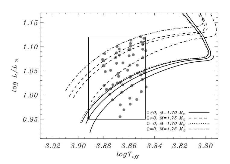
Figure 1: HR diagram containing the whole sample of models considered in this work (filled circles) as well as the observational photometric error box. Dotted and dot-dashed lines correspond to non–rotating evolutionary tracks of $1.70$ and $1.76\,{\mathrm{M}_{\odot}}$ models respectively. Continuous curves represent those of $1.70\,{\mathrm{M}_{\odot}}$ models with rotational velocities, from top to bottom, of $50$, $100$ and $150\,\rm{km}\,\rm{s}^{-1}$ respectively. Finally, dashed lines represent evolutionary tracks of $1.75\,{\mathrm{M}_{\odot}}$ models with rotational velocities varying, from top to bottom, of $50$, $100$ and $200\,\rm{km}\,\rm{s}^{-1}$ respectively.

The paper is structured as follows: In Sect. 2, fundamental parameters necessary for the modelling of Altair are given. Equilibrium models as well as our adiabatic oscillation code are described in Sect. 3. Section 4 presents a discussion of the two seismic approaches followed: 1) considering radial modes and analysing the Petersen diagrams, and 2) considering radial and non radial modes. We also discuss a possible modal identification. Finally, major problems encountered for modelling Altair and conclusions are presented in Sect. 5.

2 Fundamental parameters

Several values of the effective temperature and surface gravity of Altair ($\alpha$ Aql) can be found in the literature. Recently, (Erspamer & North, 2003) proposed $\mathrm{T}_{\mathrm{eff}}\!\!=\!\!7550\,K$ and $\log g=4.13\pm 0.3$ dex, derived from photometric measurements (Geneva system). From Hipparcos measurements (a parallax of $194.44\pm 0.94$ mas) combined with the observed V magnitude and the bolometric correction given by Flower (1996), we obtain a bolometric magnitude of $M_{\mathrm{bol}}=2.18\pm 0.1$ dex. Using previous values we thus report a luminosity of $\log(\mathrm{L/L}_{\odot})=0.984\pm 0.04$.

Rapid rotation modifies the location of stars in the HR diagram. Michel et al. (1999) proposed a method to determine the effect of rotation on photometric parameters. In the framework of $\delta$ Scuti stars, this method was then further developed by Pérez Hernández et al. (1999), showing errors around $200-300\,K$ and $0.1-0.2$ mag in the effective temperature and absolute magnitude determination respectively (see Suárez et al., 2002, for recent results on $\delta$ Scuti stars in open clusters). The error box shown in Fig. 1 has taken such systematic errors into account and it will be the reference for our modelling.

Table 2: Table containing the main characteristics of $M=1.70\,{\mathrm{M}_{\odot}}$ computed models. From left to right, $\Omega$ represents the rotational velocity in $\rm{km}\,\rm{s}^{-1}$; $\mathrm{T}_{\mathrm{eff}}$ the effective temperature (on a logarithmic scale); L/${\mathrm{L}_{\odot}}$ the luminosity in solar luminosities (on a logarithmic scale); R/${\rm{R}_{\odot}}$ the stellar radius in solar radii; $g$ the surface gravity in cgs (on a logarithmic scale); the age in Myr; $\nu(\Pi_{0})$ the frequency of the fundamental radial mode (in $\mu\mbox{Hz}$) and finally, $\Pi_{1}/\Pi_{0}$ represents the ratio between periods of the first overtone and the fundamental radial mode. Variables indexed with a $d$ represent the same quantities obtained when including near-degeneracy effects.

	$\Omega$	$\mathrm{T}_{\mathrm{eff}}$	L/L☉	R/${\rm{R}_{\odot}}$	$g$	Age	$\nu(\Pi_{0})$	$\Pi_{0}/\Pi_{1}$	$\nu(\Pi_{0}^{d})$	$(\Pi_{0}/\Pi_{1})^{d}$
m1	50	3.853	1.045	2.184	3.989	1200.0	142.553	0.772	142.504	0.772
m2	100	3.851	1.042	2.202	3.982	1192.5	140.602	0.776	139.988	0.773
m3	150	3.849	1.033	2.192	3.986	1144.2	141.355	0.782	139.176	0.760
m4	200	3.847	1.017	2.181	3.990	1039.0	141.711	0.792	141.711	0.757
m5	250	3.854	0.991	2.046	4.045	830.0	156.566	0.798	147.819	0.722
m6	50	3.859	1.038	2.112	4.018	1132.0	150.315	0.773	150.166	0.772
m7	100	3.858	1.032	2.101	4.023	1094.9	151.447	0.776	150.303	0.770
m8	150	3.858	1.020	2.079	4.032	1027.5	153.719	0.782	150.688	0.767
m9	200	3.850	1.007	2.120	4.015	959.0	148.333	0.794	141.738	0.728
m10	250	3.859	0.981	1.976	4.076	741.0	165.481	0.797	156.385	0.753
m11	50	3.867	1.026	2.007	4.062	1021.0	162.571	0.773	162.616	0.773
m12	100	3.865	1.021	2.013	4.060	999.0	161.760	0.776	162.960	0.785
m13	150	3.866	1.006	1.972	4.078	898.3	166.858	0.782	170.549	0.799
m14	200	3.859	0.993	2.001	4.065	829.0	162.627	0.792	155.581	0.758
m15	250	3.864	0.970	1.906	4.107	634.0	175.117	0.797	165.244	0.752
m16	50	3.874	1.013	1.910	4.106	899.4	175.432	0.773	175.445	0.773
m17	100	3.875	1.002	1.879	4.119	823.0	179.763	0.776	179.988	0.784
m18	150	3.873	0.990	1.872	4.123	755.7	180.692	0.782	182.011	0.805
m19	200	3.867	0.980	1.903	4.108	699.0	175.909	0.791	182.864	0.822
m20	250	3.867	0.955	1.848	4.134	509.0	183.512	0.798	190.824	0.885

Table 3: Idem Table 3 for $M=1.75{\mathrm{M}_{\odot}}$ models.

	$\Omega$	$\mathrm{T}_{\mathrm{eff}}$	L/L☉	R/${\rm{R}_{\odot}}$	$g$	Age	$\nu(\Pi_{0})$	$\Pi_{0}/\Pi_{1}$	$\nu(\Pi_{0}^{d})$	$(\Pi_{0}/\Pi_{1})^{d}$
m21	50	3.850	1.109	2.384	3.925	1211.3	126.616	0.773	126.598	0.772
m22	100	3.849	1.105	2.383	3.926	1192.5	126.544	0.776	126.205	0.771
m23	150	3.849	1.095	2.356	3.935	1144.2	128.588	0.782	126.980	0.757
m24	200	3.849	1.077	2.311	3.952	1040.0	132.064	0.792	134.845	0.765
m25	250	3.848	1.046	2.239	3.980	820.4	137.080	0.807	147.028	0.954
m26	50	3.859	1.101	2.271	3.967	1133.8	136.626	0.773	136.584	0.773
m27	100	3.859	1.094	2.248	3.976	1094.9	138.732	0.777	138.042	0.773
m28	150	3.860	1.081	2.209	3.992	1027.5	142.391	0.783	139.861	0.769
m29	200	3.859	1.062	2.167	4.008	911.0	146.203	0.792	140.219	0.735
m30	250	3.859	1.037	2.106	4.033	727.6	151.842	0.803	151.842	0.756
m31	50	3.870	1.087	2.124	4.026	1013.7	151.508	0.773	151.667	0.774
m32	100	3.868	1.082	2.135	4.021	999.0	150.273	0.777	148.854	0.769
m33	150	3.870	1.066	2.073	4.047	898.2	157.023	0.783	153.231	0.764
m34	200	3.869	1.045	2.035	4.063	768.6	161.177	0.792	154.113	0.758
m35	250	3.869	1.025	1.982	4.086	616.2	167.403	0.799	157.393	0.751
m36	50	3.880	1.071	1.991	4.082	880.3	167.222	0.773	167.240	0.773
m37	100	3.880	1.061	1.967	4.093	823.0	170.376	0.776	170.733	0.783
m38	150	3.879	1.048	1.951	4.100	755.7	172.435	0.782	174.374	0.807
m39	200	3.880	1.020	1.878	4.132	555.0	182.397	0.792	185.953	0.848
m40	250	3.878	1.012	1.878	4.133	497.4	182.263	0.796	187.153	0.866

Table 4: Idem Table 3 for $M=1.76{\mathrm{M}_{\odot}}$ models.

	$\Omega$	$\mathrm{T}_{\mathrm{eff}}$	L/L☉	R/${\rm{R}_{\odot}}$	$g$	Age	$\nu(\Pi_{0})$	$\Pi_{0}/\Pi_{1}$	$\nu(\Pi_{0}^{d})$	$(\Pi_{0}/\Pi_{1})^{d}$
m41	50	3.851	1.121	2.410	3.918	1200	124.959	0.773	124.943	0.772
m42	100	3.848	1.117	2.429	3.911	1192.5	123.249	0.776	122.984	0.771
m43	150	3.849	1.107	2.394	3.924	1144.2	125.873	0.782	124.407	0.756
m44	200	3.847	1.092	2.375	3.931	1039.0	126.768	0.793	131.618	0.874
m45	250	3.854	1.062	2.224	3.988	830.0	139.769	0.803	144.078	0.903
m46	50	3.859	1.113	2.306	3.957	1132.0	133.931	0.773	133.896	0.773
m47	100	3.859	1.106	2.285	3.965	1094.9	135.737	0.777	135.124	0.773
m48	150	3.860	1.094	2.238	3.983	1027.5	139.989	0.783	137.570	0.769
m49	200	3.857	1.083	2.248	3.979	959.0	138.644	0.791	133.851	0.736
m50	250	3.861	1.051	2.123	4.029	741.0	150.734	0.801	150.734	0.758
m51	50	3.870	1.100	2.161	4.013	1021.0	148.028	0.773	147.652	0.771
m52	100	3.868	1.095	2.165	4.012	999.0	147.557	0.777	146.313	0.770
m53	150	3.870	1.078	2.096	4.040	898.3	154.935	0.783	151.293	0.764
m54	200	3.865	1.066	2.123	4.029	829.0	151.476	0.792	145.163	0.759
m55	250	3.868	1.039	2.024	4.070	634.0	162.494	0.801	152.321	0.750
m56	50	3.879	1.085	2.031	4.067	899.4	162.756	0.773	162.782	0.773
m57	100	3.881	1.073	1.988	4.086	823.0	168.121	0.777	168.527	0.783
m58	150	3.880	1.060	1.968	4.095	755.7	170.675	0.783	172.777	0.808
m59	200	3.875	1.051	1.995	4.083	699.0	166.886	0.791	159.662	0.756
m60	250	3.873	1.021	1.944	4.105	509.0	172.969	0.802	161.557	0.749

From photometric measurements, an estimate of the mass ($1.75\pm 0.1{\mathrm{M}_{\odot}}$) and the radius ($1.58\,{\rm{R}_{\odot}}$) of the star is given by Zakhozhaj (1979); Zakhozhaj & Shaparenko (1996). However, Altair is found to rotate quite rapidly. Taking advantage of the fact that Altair is a nearby star, Richichi & Percheron (2002) measured its radius providing a diameter of 3.12 mas, which corresponds to a radius of $1.72\,{\rm{R}_{\odot}}$. Moreover, van Belle et al. (2001) showed Altair as oblate. Their interferometric observations report an equatorial diameter of $3.46$ mas (corresponding to a radius of $1.9\,{\rm{R}_{\odot}}$) and a polar diameter of 3.037 mas, for an axial ratio $a/b=1.14\pm 0.029$. The same authors derived a projected rotational velocity of ${v\!\sin\!i}=210\pm 13\,\rm{km}\,\rm{s}^{-1}$. Furthermore, Royer et al. (2002) reported ${v\!\sin\!i}$ values which range which range from $190\,\rm{km}\,\rm{s}^{-1}$ to $250\,\rm{km}\,\rm{s}^{-1}$. In addition to this, recent spectroscopically determined constraints on Altair’s inclination angle $i$ have been established by Reiners & Royer (2004). They provide a range of $i$ between 45^∘ and 68^∘, yielding therefore a range of possible equatorial velocities of Altair between $305$ and $245\,\rm{km}\,\rm{s}^{-1}$. As shown in next sections, such velocities, representing 70–90% of the break up velocity, place significant limits on our ability to model the star.

3 Modelling the star

3.1 Equilibrium models

Stellar models have been computed with the evolutionary code CESAM (Morel, 1997). Around 2000 mesh points for model mesh grid (B-splines basis) as well as numerical precision is optimized to compute oscillations.

The equation of state CEFF (Christensen-Dalsgaard & Daeppen, 1992) is used, in which, the Coulombian correction to the classical EFF (Eggleton et al., 1973) has been included. The $pp$ chain as well as the CNO cycle nuclear reactions are considered, in which standard species from ¹H to ¹⁷O are included. The species D, ⁷Li and ⁷Be have been set at equilibrium. For evolutionary stages considered in this work, a weak electronic screening in these reactions can be assumed (Clayton, 1968). Opacity tables are taken from the OPAL package (Iglesias & Rogers, 1996), complemented at low temperatures ($T\leq 10^{3}\,K$) by the tables provided by (Alexander & Ferguson, 1994). For the atmosphere reconstruction, the Eddington $T(\tau)$ law (grey approximation) is considered. A solar metallicity $Z=0.02$ is used.

Figure 2: Variation of the first overtone to fundamental radial period ratio as a function of the rotational velocity. For each mass considered, four curves are displayed, representing the results obtained modifying the effective temperature of models from $\mathrm{T}_{\mathrm{eff}}=3.85$ (bottom) to $\mathrm{T}_{\mathrm{eff}}=3.88$ (top) in steps of 0.01 dex.

Convective transport is described by the classical Mixing Length theory, with efficiency and core overshooting parameters set to $\alpha_{ML}=l_{m}/\mathrm{H}_{p}=1.8$ and $d_{ov}=l_{ov}/\mathrm{H}_{p}=0.2$, respectively. The latter parameter is prescribed by Schaller et al. (1992) for intermediate mass stars. $\mathrm{H}_{p}$ corresponds to the local pressure scale-height, while $l_{m}$ and $d_{ov}$ represent respectively the mixing length and the inertial penetration distance of convective elements.

Rotation effects on equilibrium models (pseudo rotating models) has been considered by modifying the equations (Kippenhahn & Weigert, 1990) to include the spherically symmetric contribution of the centrifugal acceleration by means of an effective gravity $g_{eff}=g-{\cal A}_{c}(r)$, where $g$ corresponds to the local gravity, and ${\cal A}_{c}(r)$ represents the radial component of the centrifugal acceleration. During evolution, models are assumed to rotate as a rigid body, and their total angular momentum is conserved.

In order to cover the range of ${v\!\sin\!i}$ given in Sect. 2, a set of rotational velocities of 50, 100, 150, 200 and $250\,\rm{km}\,\rm{s}^{-1}$ has been considered. The location in the HR diagram of models considered in this work is given in Fig. 1. A wide range of masses and rotational velocities is delimited by the photometric error box. To illustrate this, a few representative evolutionary tracks are also displayed. Characteristics of computed equilibrium models (filled circles) are given in Tables 3, 3 and 4, for models of $1.70\,{\mathrm{M}_{\odot}}$, $1.75\,{\mathrm{M}_{\odot}}$ and $1.76\,{\mathrm{M}_{\odot}}$ respectively.

3.2 The oscillation computations

Theoretical oscillation spectra are computed from the equilibrium models described in the previous section. For this purpose the oscillation code Filou (Tran Minh & L on, 1995; Suárez, 2002) is used. This code, based on a perturbative analysis, provides adiabatic oscillations corrected for the effects of rotation up to second order (centrifugal and Coriolis forces).

Furthermore, for moderate–high rotational velocities, the effects of near degeneracy are expected to be significant (Soufi et al., 1998). Two or more modes, close in frequency, are rendered degenerate by rotation under certain conditions, corresponding to selection rules. In particular these rules select modes with the same azimuthal order $m$ and degrees $\ell$ differing by 2 (Soufi et al., 1998). If we consider two generic modes $\alpha_{1}\equiv(n,\ell,m)$ and $\alpha_{2}\equiv(n^{\prime},\ell^{\prime},m^{\prime})$ under the aforementioned conditions, near degeneracy occurs for $|\sigma_{\alpha_{1}}-\sigma_{\alpha_{2}}|\leq\sigma_{\Omega}$, where $\sigma_{\alpha_{1}}$ and $\sigma_{\alpha_{2}}$ represent the eigenfrequency associated to modes $\alpha_{1}$ and $\alpha_{2}$ respectively, and $\sigma_{\Omega}$ represents the stellar rotational frequency (see Goupil et al., 2000, for more details).

Figure 3: $\Pi_{1}/\Pi_{0}$ versus $\log\!\Pi_{0}$. Three panels are displayed corresponding to the three masses considered in this work. For each panel, different lines represent the results obtained varying the rotational velocity from $\Omega=50\,\rm{km}\,\rm{s}^{-1}$ (bottom, solid line) to $\Omega=250\,\rm{km}\,\rm{s}^{-1}$ (top, dash–dotted line).

4 Comparison between theory and observations

High-amplitude $\delta$ Scuti stars (HADS) display V amplitudes in excess of 0.3 mag and generally oscillate in radial modes. In contrast, lower-amplitude members of the class present complex spectra, typically showing non-radial modes.

The amplitude of the observed main frequency is below 0.5 ppt which is several times smaller than typically detected in non-HADS $\delta$ Scuti stars from ground-based observations.

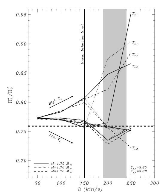
Figure 4: Same as Fig. 2 but considering near degeneracy. $T_{e,1}$ and $T_{e,2}$ labels represent effective temperatures expressed in a logarithmic scale in K. The vertical thick solid line indicates the limit for which $\Pi_{1}/\Pi_{0}$ varies linearly with $\Omega$ in presence of near degeneracy (see details in text). The horizontal dashed thick line represents the observed $\Pi_{1}/\Pi_{0}$. Finally, the shaded area represents the range of rotational velocities $\Omega$ (assuming $i=90$ deg).

As shown in paper I, using the classical period-luminosity relation with the fundamental parameters given in Sect. 2, and assuming the value of $Q=0.033\rm\leavevmode\nobreak\ d$ given by Breger (1979) for $\delta$ Scuti stars, the frequency of the fundamental radial mode is predicted to be $15.433\rm\leavevmode\nobreak\ d^{-1}$, suggestively close to the observed $f_{1}=15.768\rm\leavevmode\nobreak\ d^{-1}$. For the remaining modes (Table 1) there is no observational evidence to identify them as radial. Nevertheless, the second dominant mode, $f_{2}$, will be considered here as the first overtone.

The present study is divided into two parts. In Sect. 4.1, we consider only the two dominant modes (ie. $f_{1}$ and $f_{2}$, cf. Table 1). The observations are then compared with models through period–ratio vs. period diagrams, from now on called Petersen diagrams (see e.g. Petersen & Christensen-Dalsgaard, 1996, 1999). Then, in Sect. 4.2 we use the 5 most dominant observed modes to find the best fit to the theoretical models.

4.1 Considering two radial modes

The well known Petersen diagrams show the variation of $\Pi_{1}/\Pi_{0}$ ratios with $\log\Pi_{0}$, where $\Pi_{0}$ represents the period of the fundamental radial mode, and $\Pi_{1}$ the period of the first overtone. They are quite useful for constraining the mass and metallicity of models given the observed ratio between the fundamental radial mode and the first overtone. However these diagrams do not consider the effect of rotation on oscillations (see Petersen & Christensen-Dalsgaard, 1996, 1999, for more details). Problems arise when rapid rotation is taken into account: it introduces variations in the period ratios even for radial modes. This, combined with the sensitivity of Petersen diagrams to the metallicity, renders the present work somewhat limited. A detailed investigation of such combined effects is currently a work in progress (Suárez & Garrido, 2005). In order to cover the range of effective temperature (from $\mathrm{T}_{\mathrm{eff}}=3.85$ to $\mathrm{T}_{\mathrm{eff}}=3.88$), luminosity and rotational velocity, three sets of 20 models are computed, where rotational velocity varies from $\Omega=50$ to $\Omega=250\,\rm{km}\,\rm{s}^{-1}$. Characteristics of the three sets are given in Tables 3, 3 and 4, corresponding to sets of $1.70{\mathrm{M}_{\odot}}$, $1.75{\mathrm{M}_{\odot}}$ and $1.76{\mathrm{M}_{\odot}}$ models respectively.

Figure 5: Variation of fundamental mode frequencies $\nu(\Pi_{0})$ (in $\mu\mbox{Hz}$) with effective temperature for models with a rotational velocity of $\Omega=200\,\rm{km}\,\rm{s}^{-1}$, representative of Altair. Left panel corresponds to frequencies not corrected for the effect of near degeneracy, and right panel to those corrected. Finally, the horizontal dashed line represents the frequency of the observed fundamental mode $f_{0}^{\mathrm{obs}}$.

Adiabatic oscillations are then computed considering radial and non-radial modes. In order to analyse the Petersen diagrams corresponding to these models we calculate the $\Pi_{1}/\Pi_{0}$ ratios. In Fig. 2 the $\Pi_{1}/\Pi_{0}$ ratios are displayed as a function of the rotational velocity $\Omega$. For each mass (line style) there are four curves corresponding to four different effective temperatures (from bottom to top). It can be seen that all ratios increase proportionally with the rotational velocity. From $\Omega=50\,\rm{km}\,\rm{s}^{-1}$ to $\Omega=200\,\rm{km}\,\rm{s}^{-1}$ all models behave identically following a quasi–linear relation. For low rotational velocities, $\Pi_{1}/\Pi_{0}$ ratios approach the canonical 0.77 obtained in absence of rotation. As expected, dispersion of curves is not significant, since the masses of the models are quite similar, for a given rotational velocity. However, for $\Omega\geq 200\,\rm{km}\,\rm{s}^{-1}$, dispersion of curves also increases as a consequence of errors in the perturbative method used for computing oscillations. With rotational velocities higher than $\sim\!200\,\rm{km}\,\rm{s}^{-1}$, results should be interpreted carefully, since the second order perturbation theory considered here may fail (see Lignières, 2001, for more details). With a projected velocity of ${v\!\sin\!i}=190$–$230\,\rm{km}\,\rm{s}^{-1}$, Altair is at the limit of validity.

The impact of these results on Petersen diagrams are shown in Fig. 3. In this diagram the variation of $\Pi_{1}/\Pi_{0}$ is displayed versus $\log\Pi_{0}$ for the three masses studied. As in Fig. 2, note the trend toward the standard value of $\Pi_{1}/\Pi_{0}=0.77$ as the rotational velocity decreases. Considering the $\Pi_{1}/\Pi_{0}$ dependence in isolation, a canonical value $\Pi_{1}/\Pi_{0}(\Omega)$ can be established for a given mass. For the range of masses studied here, the analysis of three panels of Fig. 3 shows a very low dependence on mass.

Table 5: Table containing a proposed mode identification for the observed frequencies given in Table 1, using the oscillations computed from different models. Values in parentheses correspond to the mode identification numbers ($n,\ell,m$). The first five models corresponds to those chosen by their proximity to the fundamental radial mode. The last five, corresponds to those chosen by minimum $\sigma^{2}$ value. $\nu_{i}$ represent the theoretical frequencies closest to the observed ones.

	$\nu_{1}$	$\nu_{1}^{d}$	$\nu_{2}$	$\nu_{2}^{d}$	$\nu_{3}$	$\nu_{3}^{d}$	$\nu_{4}$	$\nu_{4}^{d}$	$\nu_{5}$	$\nu_{5}^{d}$	$\sigma^{2}$	$\sigma_{d}^{2}$
m18	(-1,2,0)	(1,0,0)	(1,2,2)	(1,2,2)	(2,2,-1)	(2,2,-1)	(-1,2,0)	(-1,2,0)	(-1,2,-1)	(-1,2,-1)	16.937	5.698
m19	(-2,1,0)	(1,0,0)	(3,2,2)	(3,2,2)	(4,0,0)	(4,0,0)	(-3,2,-2)	(-1,1,0)	(-1,1,-1)	(-3,2,-2)	12.531	4.056
m20	(1,0,0)	(-1,2,0)	(1,2,2)	(1,2,2)	(2,2,-1)	(2,2,-1)	(-1,2,0)	(-1,2,0)	(-1,2,-1)	(-1,2,-1)	4.575	4.544
m39	(1,0,0)	(1,1,0)	(2,2,1)	(2,2,1)	(6,2,2)	(2,2,0)	(-2,2,-1)	(-2,2,-1)	(-2,2,-1)	(-2,2,-1)	21.234	7.600
m40	(1,0,0)	(-1,2,-2)	(1,2,0)	(1,2,0)	(3,1,1)	(3,1,1)	(-1,2,-2)	(-1,2,-2)	(1,1,1)	(1,1,1)	0.763	1.242
m10	(-1,1,0)	(-2,2,0)	(3,2,2)	(3,2,2)	(4,0,0)	(4,0,0)	(-3,2,-2)	(-1,1,0)	(-1,1,-1)	(-3,2,-2)	1.194	0.820
m13	(-1,2,0)	(-1,2,0)	(1,2,2)	(1,2,2)	(2,2,-1)	(2,2,-1)	(-1,2,0)	(-1,2,0)	(-1,2,-1)	(-1,2,-1)	0.903	0.903
m23	(-1,2,-2)	(-1,2,-2)	(3,2,2)	(3,2,2)	(4,1,-1)	(4,1,-1)	(0,2,0)	(0,2,0)	(0,2,0)	(0,2,0)	0.835	0.835
m34	(-1,2,0)	(1,1,0)	(2,2,1)	(2,2,1)	(6,2,2)	(2,2,0)	(-2,2,-1)	(-2,2,-1)	(-2,2,-1)	(-2,2,-1)	1.698	1.228
m58	(-1,2,-2)	(-1,2,-2)	(2,1,1)	(2,1,1)	(3,1,-1)	(3,1,-1)	(-1,1,1)	(-1,1,1)	(1,1,1)	(1,1,1)	0.639	0.940

Up to this point, the effect of near degeneracy has not been taken into account. Near degeneracy occurs systematically for close modes (in frequency) following certain selection rules (see Sect. 3.2). It increases the asymmetry of multiplets and thereby the behaviour of modes. The higher the value of the rotational velocity, the higher the importance of near degeneracy. In the present case, for the range of rotational velocities considered, near degeneracy cannot be neglected. As can be seen in Fig. 4, not all models present the same behaviour with $\Omega$. For rotational velocities up to $150\,\rm{km}\,\rm{s}^{-1}$, a double behaviour is shown, one for lower effective temperatures ($\Pi_{1}^{d}/\Pi_{0}^{d}<0.77$), and one for higher effective temperatures ($\Pi_{1}^{d}/\Pi_{0}^{d}>0.77$), both remaining linear. This shows the dependence of $\Pi_{1}/\Pi_{0}(\Omega)$ with the evolutionary stage of the star. However, for higher rotational velocities, particularly on the right side of the vertical limit line, everything becomes confusing. At these rotational velocities, the global effect of rotation up to second order (which includes asymmetries and near degeneracy) on multiplets complicates the use of $\Pi_{1}^{d}/\Pi_{0}^{d}(\Omega)$ predictions on a Petersen diagram. In particular, radial modes are affected by rotation through the distortion of the star (and thereby its propagation cavity), and through near degeneracy effects, coupling them with $\ell=2$ modes (Soufi et al., 1998). In addition, other factors such as the evolutionary stage and the metallicity must also be taken into account, which makes the global dependence of Petersen diagrams on rotation rather complex.

In Fig. 5 (left and right panels), the combined effect of rotation and evolution on the fundamental radial mode is shown for representative models with a rotational velocity of $200\,\rm{km}\,\rm{s}^{-1}$. In particular, for the $1.76\,{\mathrm{M}_{\odot}}$ model, the stellar radius is approximately $10^{-1}\,{\rm{R}_{\odot}}$ larger than those of $1.70$ and $1.75\,{\mathrm{M}_{\odot}}$, which difference is of the order of $10^{-2}\,{\rm{R}_{\odot}}$. As a result, a clear difference of behaviour between those models is observed. Such a difference depends not only on the mass, but also on the evolutionary stage, the inital rotational velocity (at ZAMS), metallicity, etc. In Suárez et al. (2005), for a certain small range of masses, a similar non-linear behaviour is found for predicted unstable mode ranges. The results of this work may provide a clue to understand this unsolved question.

The reader should notice that at these velocities, when frequencies are corrected for near degeneracy effects, their variations with $\mathrm{T}_{\mathrm{eff}}$ (and thereby with evolution) are more rapid (right panel) than was the case for uncorrected ones. Moreover, a shift to higher frequencies is observed when correcting for near degeneracy, which favors the selection of lower mass objects. For low temperatures (i.e. for more evolved models), stabilization is found for low $\nu(\Pi_{0}^{d})$ frequencies, which can be explained by the joint action of both near degeneracy and evolution effects.

In the present work, following the prescription of Goupil et al. (2000), modes are near degenerate when their proximity in frequency is less or equal to the rotational frequency of the stellar model ($|\nu_{i}-\nu_{j}|\lesssim\sigma_{\Omega}$). Considering all possibilities, 5 models identify the observed $f_{1}$ as the fundamental radial mode: m₁₈, m₁₉, m₂₀ ($1.70\,{\mathrm{M}_{\odot}}$), m₃₉ and m₄₀ ($1.75\,{\mathrm{M}_{\odot}}$). For last three models (20, 39 and 40), this happens without considering near degeneracy effects. For m₁₈ and m₁₉, the theoretical fundamental mode approaches $f_{1}$ when considering near degeneracy.

In Table 5, radial and non radial identifications (discussed in the next section) are presented for selected models. The first set of five models corresponds to those selected by their identification of $f_{1}$ as the radial fundamental mode. As can be seen, no identification is possible when trying to fit the whole set of observed frequencies. However $f_{3}$ is identified as the third overtone by the rapid rotating model ($\Omega=200\,\rm{km}\,\rm{s}^{-1}$) m₁₉. Uncertainties in the observed mass and metallicity are also an important source of error in determining the correct equilibrium model. Thus, the fact of obtaining fundamental modes with frequencies lower than $180\,\mu\mbox{Hz}$ for most of the models could be explained by an erroneous position of the photometric box on the HR diagram. In fact, the lower the mass of model used (always within the errors), the higher the $\nu(\Pi_{0})$ value. However, the location in the HR diagram of models with masses lower than $1.70\,{\mathrm{M}_{\odot}}$ (with the same metallicity) is not representative of the Altair observations.

At this stage, there are two crucial aspects to fix. On one hand, it is necessary to determine the physical conditions which enforce degeneracy between mode frequencies. A physically selective near–degeneracy could explain the behaviour of $\Pi_{1}/\Pi_{0}$ for very high rotating stars. On the other hand, for high rotational velocities, third order effects of rotation are presumably important.

4.2 Non-radial modes.

As neither observational nor theoretical evidence supporting a radial identification of the observed modes $f_{j}$ exists, in this part of the work, we carry out an analysis generalised to non-radial modes. As we did for radial oscillations (see Sect. 3.2), here we compute non-radial adiabatic oscillations for the models of Tables 3, 3 and 4. Assuming the 7 observed modes of Altair pulsate with $\ell\leq 3$, a possible mode identification is proposed in Table 5. In order to avoid confusion, only the first 5 observed modes (Table 1) with larger amplitudes, will be considered. This constitutes a rough identification based only on the proximity between observed and theoretical mode frequencies for each model. That is, no additional information about the $\ell$ and $m$ values is used.

In order to obtain an estimate of the quality of fits (identification of the whole set of observed frequencies), the mean square error function is used. The lower its value, the better the fit for the free parameters considered. For each model

$$\sigma^{2}=\frac{1}{N}\sum_{i=1}^{N}\,\Big{(}f_{o,i}-\nu_{t,i}\Big{)}^{2}$$ (1)

is calculated, where $f_{o,i}$ and $\nu_{t,i}$ represent the observed and theoretical frequencies respectively. The total number of observed frequencies is represented by $N=5$. Calculations are made fixing the metallicity $Z$, the overshooting parameter $d_{\mathrm{ov}}$ and the mixing length parameter $\alpha_{\mathrm{ML}}$ (see Sect. 3.1). On the other side, the mass M, the rotational velocity $\Omega$ and the evolutionary stage $X_{c}$ have been considered as free parameters. In Table 5, the last two columns list $\sigma^{2}(\mathrm{M},\Omega,X_{c})$ calculated for each model, both without near degeneracy ($\sigma^{2}$) and including it ($\sigma_{d}^{2}$). When considering the whole set of models computed, the inclusion of near degeneracy increases the quality of fits by roughly 30%.

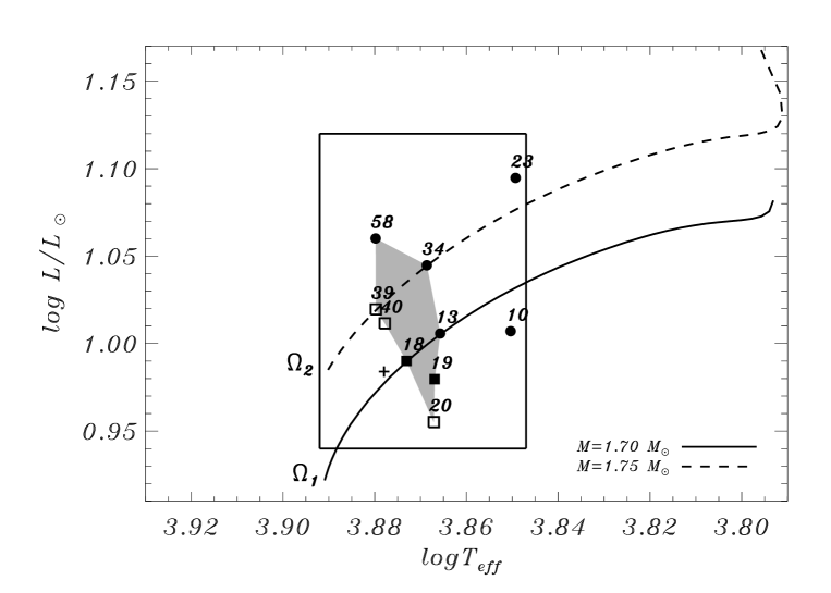
Figure 6: HR diagram showing selected models given in Table 5. Labels correspond to model numbers. Square symbols represent models selected by the proximity to the fundamental radial mode; filled squares are used for those taking into account near degeneracy effects. Filled circles represent models selected by the minimum $\sigma^{2}$ value. As a reference, observations (the cross symbol) and two evolutionary tracks are depicted: One corresponding to a $1.70\,{\mathrm{M}_{\odot}}$ and $\Omega_{1}=150\,\rm{km}\,\rm{s}^{-1}$ (solid line), and the other one, corresponding to a $1.75\,{\mathrm{M}_{\odot}}$ and $\Omega_{2}=200\,\rm{km}\,\rm{s}^{-1}$ (dashed line). For more details see the text.

Table 5 is divided in two parts: the first 5 models have been chosen as identifying $f_{1}$ as the fundamental radial mode. The second set of models correspond to those with minimizing $\sigma^{2}$. Analysing the results obtained for the 14 selected models it can be seen that no $\ell=3$ identifications are found and most of identifications correspond to $\ell=2$ ( 60%) and $\ell=1$ ( 32%) modes. As happened for the first set of models, $f_{3}$ is identified as the third radial overtone by models m₁₀.

On the other hand, since no specific clues for the degree $\ell$ and the azimuthal order $m$ are given, other characteristics of the observed spectrum must be investigated. In particular, it is quite reasonable to consider some of the observed frequencies as belonging to one or more rotational multiplets. Although no complete multiplets are found, several sets of two multiplet members are obtained. Specifically, the observed frequencies $f_{4}$ and $f_{5}$ are identified as members of $\ell=2$ multiplets by models m₁₃, m₁₈, m₂₀, m₃₉ and m₁₀, and as members of $\ell=1$ triplets by models m₁₀ and m₁₉.

Figure 6 shows the location on a HR diagram of selected models given in Table 5. Notice that around 80% of them lie in effective temperature and luminosity ranges of $\log\mathrm{T}_{\mathrm{eff}}=[3.88,3.85]$ and $\log\mathrm{L/}{\mathrm{L}_{\odot}}=[0.96,1.09]$ respectively. In the area delimited by these models (shaded surface), models with similar characteristics are found. As can be seen, the shaded area is located in the central part of the error box. Except models m₃₉, m₄₀ and m₅₈, all models are situated toward colder and more luminous locations in the box. This is in agreement with the expected effect of rotation on fundamental parameters (see Sect. 2). On the other hand, positions of models selected by the proximity to the fundamental radial mode (squares) can be connected by a straight line. This is an iso-${\bar{\rho}}$ line, with ${\bar{\rho}}\simeq 5.23\,\rm{g}\,\rm{cm}^{3}$, and which basically explains the similar frequencies of their fundamental radial mode. Considering near-degeneracy, the identification of the fundamental radial mode and the lowest $\sigma^{2}$ value, our best model is m₁₉, which is at the lower limit of the range of Altair’s observed ${v\!\sin\!i}$.

Nevertheless, in order to further constrain our models representative of Altair, it would be necessary to obtain additional information on the mode degree and/or azimuthal order of observations. In this context, spectroscopic analysis may provide information about $\ell$, $m$ and the angle of inclination of the star, as nonradial pulsations generate Doppler shifts and line profile variations (Aerts & Eyer, 2000). Furthermore, multicolor photometry may also provide information about $\ell$ (Garrido et al., 1990).

5 Conclusions

In the present paper a theoretical analysis of frequencies of HR6534 (Altair) was presented, where rapid rotation has been properly taken into account in the modelling. The analysis was separated in two parts: 1) considering the observed modes $f_{1}$ and $f_{2}$ corresponding to the fundamental radial mode and the first overtone and models were analysed through the Petersen diagrams, and 2) a preliminary modal identification was proposed by considering radial and non-radial oscillations.

Firstly, in the context of radial modes, we studied the isolated effect of rotation on Petersen diagrams. For the different rotational velocities considered, the shape of $\Pi_{1}/\Pi_{0}(\Omega)$ leads to a limit of validity of the perturbation theory (up to second order) used at around $\Omega=200\,\rm{km}\,\rm{s}^{-1}$. This limit is mainly given by the behaviour of such period ratios when near degeneracy is considered, which visibly complicates the interpretation of Petersen diagrams. Nevertheless, in this procedure, for rotational velocities up to $150\,\rm{km}\,\rm{s}^{-1}$ it is found that $\Pi_{1}/\Pi_{0}$ is lower than 0.77 for lower effective temperatures, and reciprocally higher than 0.77 for higher effective temperatures (inside the photometric error box). The analysis of radial modes also reveals that only a few models identify the observed $f_{1}$ as the fundamental radial mode. This reduces the sample of models to those with masses around $1.70\,{\mathrm{M}_{\odot}}$ or lower, on the main sequence and implies models with different metallicity in order to agree with photometric error box. These partial results (for a given region in the HR diagram, for a given range of masses, evolutionary stages and a given metallicity) constitute a promising tool for seismic investigation, not only of $\delta$ Scuti stars, but in general, of multi-periodic rotating stars. A detailed investigation on the effect of both rotation and metallicity on Petersen diagrams will be proposed in a coming paper (Suárez & Garrido, 2005).

Secondly, in the context of radial and non radial modes and assuming observed modes pulsating with $\ell=0,1,2,3$, a set of 14 models was selected in which five of them identify the fundamental radial order and at least six others identify two of the observed frequencies ($f_{4}$ and $f_{5}$) as members of $\ell=2$ and $\ell=1$ multiplets. A range of masses of [1.70,1.76] ${\mathrm{M}_{\odot}}$ principally for a wide range of evolutionary stages on the main sequence (ages from 225 to 775 Myr) was obtained. Considering information of both radial (through Petersen diagrams) and non-radial modes, a set of representative models with rotational velocities larger than $150\,\rm{km}\,\rm{s}^{-1}$ was obtained.

Further constraints on the models are thus necessary. Such constraints can be obtained by employing additional information on the mode degree $\ell$ and/or the azimuthal order $m$ of the observed modes, which may be inferred from spectroscopy and multicolor photometry (Garrido et al., 1990). Improvements on adiabatic oscillation computations (including third order computations) will constitute a coherent and very powerful tool to obtain seismic data from future space missions like COROT, EDDINGTON and MOST.