A new calibration of stellar parameters of Galactic O stars

We present new calibrations of stellar parameters of O stars at solar metallicity taking non-LTE, wind, and line-blanketing effects into account. Gravities and absolute visual magnitudes are derived from results of recent spectroscopic analyses. Two types of effective temperature scales are derived: one from a compilation based on recent spectroscopic studies of a sample of massive stars – the “observational scale” – and the other from direct interpolations on a grid of non-LTE spherically extended line-blanketed models computed with the code CMFGEN (Hillier & Miller hm98 (1998)) – the “theoretical scale”. These $T_{\mathrm{eff}}$ scales are then further used together with the grid of models to calibrate other parameters (bolometric correction, luminosity, radius, spectroscopic mass and ionising fluxes) as a function of spectral type and luminosity class. Compared to the earlier calibrations of Vacca et al. (vacca (1996)) the main results are:

• The effective temperature scales of dwarfs, giants and supergiants are cooler by 2000 to 8000 K, the theoretical scale being slightly cooler than the observational one. The reduction is the largest for the earliest spectral types and for supergiants.

• Bolometric corrections as a function of $T_{\mathrm{eff}}$ are reduced by 0.1 mag due to line blanketing which redistributes part of the UV flux in the optical range. For a given spectral type the reduction of $BC$ is larger for early types and for supergiants. Typically $BC$s derived using the theoretical $T_{\mathrm{eff}}$ scale are 0.40 to 0.60 mag lower than that of Vacca et al. (vacca (1996)), whereas the differences using the observational $T_{\mathrm{eff}}$ scale are somewhat smaller.

• Luminosities are reduced by 0.20 to 0.35 dex for dwarfs, by $\sim$ 0.25 for all giants and by 0.25 to 0.35 dex for supergiants. The reduction is essentially the same for both $T_{\mathrm{eff}}$ scales. It is independent of spectral type for giants and supergiants and is slightly larger for late type than for early type dwarfs.

• Lyman continuum fluxes are reduced. Our theoretical values for the hydrogen ionising photon fluxes for dwarfs are 0.20 to 0.80 dex lower than those of Vacca et al. (vacca (1996)), the difference being larger at late spectral types. For giants the reduction is of 0.25 to 0.55 dex, while for supergiants it is of 0.30 to 0.55 dex. Using the observational $T_{\mathrm{eff}}$ scale leads to smaller reductions at late spectral types.

The present results should represent a significant improvement over previous calibrations, given the detailed treatment of non-LTE line-blanketing in the expanding atmospheres of massive stars.

1 Introduction

Despite their paucity, massive stars play a crucial role in several fields of astrophysics: they enrich the interstellar medium in heavy elements; they create H ii regions; they release huge quantities of mechanical energy through their winds; they explode as supernovae; they are possibly at the origin of Gamma-Ray Bursts; and the first massive stars may have reionised the early Universe at redshift beyond 6. Hence, a good knowledge of their properties is crucial and requires the development of both evolutionary and atmosphere models.

Three main ingredients have to be included in massive stars atmospheres: a full non-LTE treatment since radiative processes are dominant over thermal processes (e.g. Auer & Mihalas am72 (1972)); spherical expansion due to the stellar wind and the related velocity fields (Hamann hamann86 (1986), Hillier 1987a , 1987b , Gabler et al. gabler89 (1989), Kudritzki kud92 (1992), Najarro et al. paco96 (1996)); and line-blanketing to take into account the effects of metals on the atmospheric structure and emergent spectrum (Abbott & Hummer ah85 (1985), Schaerer & Schmutz ss94 (1994)). The two former ingredients were the first to be included in the models, but it is only recently that line-blanketing has been handled reliably. The main reason is the complexity of the problem which has to be solved when thousands of level populations from metals have to be computed through the resolution of statistical equilibrium and radiative transfer equations in an expanding medium. Various solutions have been developed to include line-blanketing: opacity sampling method in the code WM-BASIC (Pauldrach et al. wmbasic01 (2001)), approximate method to estimate line-blocking and blanketing in FASTWIND (Santolaya-Rey et al. fast97 (1997), Puls et al. puls05 (2005)), opacity distribution functions in TLUSTY (Hubeny & Lanz hl95 (1995), Lanz & Hubeny ostar2002 (2002)), or comoving frame calculations using super-levels in CMFGEN (Hillier & Miller hm98 (1998)). Each method and code has its advantages and disadvantages: WM-BASIC makes a treatment in the observer’s frame uising a Sobolev plus continuum approximation in the solution of the rate equations and does not include line broadening terms, but makes a complete hydrodynamical calculation of the atmosphere structure; FASTWIND is designed for fast computations but makes only an approximate treatment of opacities from metals for which no line profile is (yet) predicted; TLUSTY makes a very detailed calculation of the NLTE rate equations but is limited to plane-parallel geometry; finally, CMFGEN solves the NLTE rate equations in the comoving frame but uses super-levels.

The effects of line-blanketing on atmosphere models lead to quantitative modifications of the stellar and wind properties of massive stars in general and O stars in particular. The most studied effect is the reduction of the effective temperature scale (Martins et al. teffscale (2002), Crowther et al. paul02 (2002), Herrero et al. hpn02 (2002), Bianchi & Garcia bg02 (2002), Repolust et al. repolust (2004), Massey et al. massey04 (2004)). Indeed, the increased number of diffusions in the inner atmosphere due to metallic line opacities implies a heating of the deeper layers (backwarming effect) and consequently a higher ionisation which shifts the relation between effective temperature and spectral type. The reduction can be as high as 7000 K for extreme supergiants (Crowther et al. paul02 (2002)). Such a change of the effective temperatures implies lower luminosities and lower ionising fluxes, which is crucial for studies involving H ii regions and star forming regions.

A good knowledge of the effective temperature scale of O stars is fundamental since $T_{\mathrm{eff}}$ cannot be derived from optical photometry: the visual spectrum of O stars is in the Rayleight-Jeans part of the distribution and is thus almost insensitive to $T_{\mathrm{eff}}$. Several $T_{\mathrm{eff}}$ scales have been proposed in the past (Conti conti73 (1973), Schmidt-Kaler sk82 (1982)) based on models without winds and metals, the most recent one being that of Vacca et al. (vacca (1996)). As these ingredients are now available in models, revisions of such calibrations are possible. Once obtained, they can be used to calibrate other important parameters such as luminosities and ionising fluxes.

Two main approaches lend themselves to derive a temperatures scale as a function of spectral type (hereafter ST) and luminosity class (LC): 1) the determination of average $T_{\mathrm{eff}}$’s from an observed sample of O stars, or 2) the determination of $T_{\mathrm{eff}}$’s from the comparison of extended model atmosphere grids with the observed mean properties defining the spectral types, i.e. He i/He ii spectral line ratios for O stars. Both methods, hereafter referred to as the “observational scale” (1) and the “theoretical scale” (2) , are employed in the present work. Their advantages and drawbacks are roughly the following. Obviously the establishment of an “observational scale” relies on a sufficient and representative number of individual stars of all spectral types and luminosity classes, which have been analysed with state-of-the-art non-LTE line blanketed model atmospheres with stellar winds. Several such studies have been pursued in the last years (Crowther et al. paul02 (2002), Herrero et al. hpn02 (2002), Hillier et al. hil03 (2003), Bouret et al. jc03 (2003), Repolust et al. repolust (2004), Markova et al. mark04 (2004), Evans et al. evans04 (2004), Martins et al. 2004a , wwgal (2005)). However, the parameter space of O stars covered by these studies based on non-LTE, line blanketed models with winds remains only partly sampled. This problem can be alleviated by the computation of a grid of models covering the whole range of parameters from which “theoretical calibrations” can be derived. However, as in principle the parameter space – accounting e.g. for $\dot{M}$, the velocity law, microturbulence and others – is rather large, assumptions have to be made on the adopted input parameters or combinations thereof. Finally, these models can also be tested by comparison to observational results from individual stars. Given these advantages and limitations we have chosen to use both approaches to establish a new $T_{\mathrm{eff}}$ scale and to examine their implications on the recalibration of the remaining stellar parameters.

In Sect. 2 we describe the atmosphere models; we present the sample of observed stars from which we have derived estimated spectroscopic gravities and absolute visual magnitudes of dwarfs, giants and supergiants in Sect. 3; in Sect. 4 we explain our method to derive the effective temperature scales; in Sect. 5, we show the results of the calibrations of other stellar parameters (bolometric correction, luminosity, radius, mass, ionising flux); in Sect. 6 we discuss the effect of metallicity on the present results and the conclusions are gathered in Sect. 7.

2 Modelling

We have constructed a grid of models for O stars using the atmosphere code CMFGEN (Hillier & Miller hm98 (1998)). We have tried to sample as well as possible the $\log g$–$T_{\mathrm{eff}}$ plane in order to cover the whole range of spectral types and luminosity classes. In practice, we have relied on the grid of CoStar models of Schaerer & de Koter (costar3 (1997)): models A2$\rightarrow$E2, A3$\rightarrow$E3 and A4$\rightarrow$D4 have been recomputed with the same set of parameters as in the original grid. In addition, we have computed new models to refine this grid: after adopting $T_{\mathrm{eff}}$ and $\log g$, we have derived $\log\frac{L}{L_{\odot}}$ from the evolutionary tracks at solar metallicity of Meynet et al. (1994), which lead to $R$ and then $M$ through $\log g$; the terminal velocity ($v_{\infty}$) was chosen to be 2.6 time the escape velocity (see Lamers et al. lamers95 (1995), Kudritzki & Puls kp00 (2000)) and the mass loss rate was computed according to the cooking recipe of Vink et al. (vink01 (2001)). A total of 38 models with $3.0<\log g<4.25$ and $25000<T_{\rm eff}\ <48000$ K was finally computed.

The main characteristics of CMFGEN are largely described by Hillier & Miller (hm98 (1998)). We give here a short overview:

- Non-LTE: all statistical equilibrium equations are solved individually to provide the detailed level populations. The radiative transfer equation is also solved and leads to the radiation field.

- Line-blanketing: line-blanketing is included directly by means of a super-level approach. In addition to H and He, C, N, O, Si, S and Fe level populations have been computed in our models. This amounts to $\sim$ 2000 levels and $\sim$ 800 super-levels. Solar abundances according to Grevesse & Sauval (gs98 (1998)) have been adopted. Numerous tests have been undertaken to confirm the accuracy of the super-level approach. While the strength of individual lines can be affected by using too few super-levels, or by poor super-level assignments, the method provides consistent non-LTE blanketed structures. Moreover, the super-level assignments are easily changed, and are often simply used to group levels of the same LS configuration. Note that the adopted super-level approach does not directly influence line blanketing: its influence is indirect, and arises through its effect on the non-LTE level populations obtained from the solution of the statistical equilibrium equations

- Temperature: the temperature structure is derived from the radiative equilibrium equation.

- Hydrodynamical structure: CMFGEN does not compute self-consistently the hydrodynamical structure which has to be given as input and which is held fixed. We have adopted the velocity structure resulting from the smooth connection by smooth connection, we mean that both the velocity $v(r)$ and its derivative $dv/dr$ are imposed to be continuous at the connecting point. of a pseudo-hydrostatic photospheric velocity structure with the $\beta$-law ($v=v_{\infty}(1-\frac{R}{r})^{\beta}$) representing the wind (with a value of $\beta$ chosen to be 0.8). The photospheric structure was taken from the TLUSTY grid of models OSTAR2002 (Lanz & Hubeny ostar2002 (2002)). Fig. 1 shows the initial TLUSTY structure (dashed line) together with the CMFGEN input structure (solid line) in a typical case. One sees that the transition between the TLUSTY hydrostatic structure and the CMFGEN “wind” structure corresponds to a velocity of the order of a few km s^-1 (or typically 10 to 30 $\%$ of the sound speed) which ensures that the important effects of velocity fields and spherical expansion are taken into account even in the photosphere (e.g. Kudritzki kud98 (1998)). Note also that the density at the connecting point scales with the mass loss rate, so that the adopted wind structure has most effects in supergiant models. When the parameters $T_{\mathrm{eff}}$–$\log g$ did not match any of the TLUSTY models, we have simply linearly interpolated the photospheric velocity structure from the closest neighbours in the OSTAR2002 grid (see also Martins et al. wwgal (2005)). For example for a model with temperature $35000<T_{\rm eff}\ <40000$ K, we estimated the density and optical depth from the TLUSTY models with $T_{\mathrm{eff}}$ = 35000 and 40000 K according to $x=\frac{T_{\rm eff}-35000}{40000-35000}*(x40-x35)+x35$ where $xi$ is the density or optical depth at temperature $i$ in kK. This method, although approximate, was tested by Bouret et al. (jc03 (2003)) and was found to give the same structure as a true computation with TLUSTY.

- Microturbulent velocity: a microturbulent velocity can be included in the models. In the computation of the atmospheric structure (level populations, radiation field), we have chosen a value of 20 km s^-1 while in the computation of the formal solution of the radiative transfer leading to the detailed emergent spectrum, we have adopted $v_{turb}$ = 5 km s^-1. The quite high value used in the atmospheric structure is required to avoid extremely long computation time. Test models have revealed that the He i $\lambda$4471  and He ii $\lambda$4542  line profiles were basically unaffected by a decrease of $v_{\rm turb}$ from 20 km s^-1 to 10 km s^-1 in the atmosphere structure calculation (see Martins et al. 2004a , Martins et al. wwgal (2005)). Note also that microturbulent velocities of 10 to 20 km s^-1 are often found when modelling supergiants (e.g. hillier et al. hil03 (2003)).

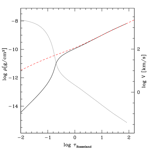
Figure 1: Typical hydrodynamical structure: density as a function of Rosseland optical depth for a model with $T_{\mathrm{eff}}$ = 40000 K, $\log g$ = 3.50 and $\dot{M}$ = $1.410^{-5}$ M_⊙/yr. The red dashed line is the initial TLUSTY structure on which a $\beta$ velocity law is connected to give the final CMFGEN input structure (black solid line). The dotted line shows the CMFGEN velocity structure as a function of Rosseland optical depth. The TLUSTY and CMFGEN structures are similar in the very inner atmosphere and start to depart from each other around $\log\tau_{Rosseland}\sim 0$ which corresponds to a velocity of a few km s^-1.

3 Observed sample

We have compiled the results from optical spectroscopic analysis of Galactic O stars using non-LTE spherically expanding models including line-blanketing. In practice, we have used the results of the studies of Herrero et al. (hpn02 (2002)) and Repolust et al. (repolust (2004)) based on models computed with FASTWIND. We have also used our own results from the analysis of Galactic O dwarfs with CMFGEN (Martins et al. wwgal (2005)) so that the number of O stars in this observed sample amounts to 45 objects. We have not included the results of Markova et al. (mark04 (2004)) since most of the stellar parameters where derived from calibrations and not from analysis with atmosphere models. We also excluded objects analysed by Bianchi & Garcia (bg02 (2002)) and Garcia & Bianchi (gb04 (2004)) since their studies are based on pure UV analysis and yield quite discrepant results to optical and combined UV-optical analysis for reasons we discuss now.

The above mentioned pure UV analysis (using WM-BASIC) relied on two main $T_{\mathrm{eff}}$ indicators, O v $\lambda$1371  and P v $\lambda\lambda$1118,1128 , lines which strongly depend on the wind properties (in particular clumping, see Crowther et al. paul02 (2002), Bouret et al. jc05 (2005)). Moreover, WM-BASIC does not allow a treatment of Stark broadening which is crucial to correctly predict the width of gravity sensitive lines which are moreover essentially absent in the UV range. Note that the effects of clumping should not directly modify the present results, since we use photospheric lines formed well below the radius where clumping appears. In spite of this, we can not discard the fact that UV $T_{\mathrm{eff}}$ diagnostics sometimes lead to lower values than optical lines, as is the case of the WM-BASIC studies of Bianchi & Garcia (bg02 (2002)) and Garcia & Bianchi (gb04 (2004)). However, other recent analysis show that consistent results with good fits can be obtained for photospheric UV and optical lines (Bouret et al. jc03 (2003), Hillier et al. hil03 (2003), Martins et al. wwgal (2005)). Given this, and since our present approach is based on $T_{\mathrm{eff}}$- sensitive optical He lines, we do not include the results of spectroscopic analysis based only on UV non-photospheric lines in our observational sample.

4 Gravities and effective temperatures

As gravity is the main parameter determining the luminosity class a calibration of this quantity is needed to allow the calibration of effective temperature for different LC. Once established, such a $\log g$–ST relation for all LC can be used in the model atmosphere grid to produce new relations between effective temperature and spectral type, using gravity to discriminate between luminosity classes. These steps, as well as the determination of the observational $T_{\mathrm{eff}}$ scale are now discussed.

All the resulting calibrated stellar parameters are summarised in Tables 1 to 6.

4.1 $\log g$–ST relation

The observational sample including recent spectroscopic analysis of individual stars has been used to derived an empirical calibration $\log g$–ST. Note that the gravities used here are corrected for the effect of rotation, except for the dwarfs stars studied by Martins et al. (wwgal (2005)). However in the latter study, the rotational velocities are not larger than 130 km s^-1 so that the difference between derived $\log g$ and “true” $\log g$ is negligible (see e.g. Repolust et al. repolust (2004)). The results are shown in Fig. 2 where dwarfs are represented by triangles, giants by squares and supergiants by circles. We note that there is a significant scatter in the empirical points leading to standard deviations of 0.15, 0.07 and 0.12 dex respectively for dwarfs, giants and supergiants. The linear fits are to the observational results for dwarfs, giants and supergiants are:

$$\log g=\left\{\begin{array}[]{l}3.924-0.001\times\textrm{ST \hskip 28.45274pt (V)}\\ 3.887-0.040\times\textrm{ST \hskip 28.45274pt (III)}\\ 3.979-0.083\times\textrm{ST \hskip 28.45274pt (I)}\end{array}\right.$$ (1)

where $ST$ is the spectral type.

Vacca et al. (vacca (1996)) established a relation between spectroscopic gravities and spectral type from results of spectroscopic analysis through plane-parallel pure H He non-LTE models. We have proceeded similarly except that we have relied on atmosphere models including also winds and line-blanketing. Figure 2 (upper panel) shows the differences between the two calibrations for various luminosity classes. We see that they are very close, the difference being less than 0.1 dex, which is the typical error generally quoted for the determination of spectroscopic gravities from the fit of Balmer lines. Herrero et al. (hpv00 (2000)) showed that the inclusion of winds in atmosphere models lead to a systematic increase of $\log g$ by 0.1 to 0.25 dex. The present results show that on average gravities derived with plane parallel H He models are similar to those derived with line blanketed spherically extended models. Note that the results of Herrero et al. (hpv00 (2000)) are for supergiants with strong winds ($\dot{M}$ of the order of $10^{-5..-6}$ M_⊙/yr) for which an effect of the wind on the $\log g$ sensitive lines is not unexpected. For stars with such high density winds, the lowering of $T_{\mathrm{eff}}$ imposed by the inclusion of line-blanketing may compensate for this wind effect so that, fortuitously, the relation $\log g$ – ST is not significantly changed.

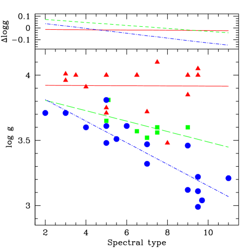
Figure 2: Lower panel: gravity as a function of spectral type. Symbols corresponds to results derived from spectroscopic analysis of observed Galactic stars (sources: Repolust et al. repolust (2004), Herrero et al. hpn02 (2002) and Martins et al. wwgal (2005)). Triangles are dwarfs, squares are giants and circles are supergiants. Lines are the least square fits of the observational data (solid: dwarfs; dashed: giants; dot-dashed: supergiants). Upper panel: difference between the calibration of Vacca et al. (vacca (1996)) and the present ones.

4.2 $T_{\mathrm{eff}}$scales

As already discussed, the derivation of new effective temperature scales was made following two different methods: First, the relation between spectral type and $T_{\mathrm{eff}}$ was derived directly from our grid of models, using the above $\log g$– ST relation to discriminate between luminosity classes (“theoretical scale”). Second, we used the sample of stars analysed with quantitative spectroscopy to estimate the mean relation $T_{\mathrm{eff}}$–ST (“observational scale”). The resulting calibrated stellar parameters using the theoretical $T_{\mathrm{eff}}$ scale are summarised in Tables 1 to 3, those based on the observational $T_{\mathrm{eff}}$ scale in Tables 4 to 6.

4.2.1 $T_{\mathrm{eff}}$ scale from models (“Theoretical scale”)

Here, we show how we derived new $T_{\mathrm{eff}}$ scales from our grid of models. The advantage of using models is that we can sample the whole spectral and luminosity range. However, the results depends on the grid of model and the parameters adopted to compute these models.

The basic idea is to build a function $T_{\mathrm{eff}}$(ST,$\log g$) from which temperatures from dwarfs, giants and supergiants — characterised by a given relation $\log g$–ST — were derived. For this, we have made 2D interpolations using the NAG routines e01sef and e01sff. The basic principle of such routines is to construct a surface $T_{\mathrm{eff}}$($\log g$,ST) regularly sampled in $\log g$–$T_{\mathrm{eff}}$from the grid model points (not regularly sampled in the space parameter) and then to determine the effective temperatures from this surface for a given $\log g$–ST relation. The construction of the surface involves two parameters representing basically the number of neighbouring input points from which we want the interpolation to be made for a given ($\log g$,$T_{\mathrm{eff}}$) of the regular grid. We have tested the effects of a change of the values of these parameters on our results and have found that for a reasonable number of neighbouring points ($>$ 15) there was essentially no modification. Note that we have not used directly the spectral type as a parameter, but we rely on the ratio of the equivalent widths $\log(EW(HeI\lambda 4471)/EW(HeII\lambda 4542))\equiv\log W^{\prime}$), which is directly related to ST through the classification scheme of Mathys (mathys88 (1988)). According to this scheme, a given spectral type corresponds to a range of values for $W^{\prime}$ so that all stars having $W^{\prime}$ in this range will have the same spectral type, introducing thus a dispersion in any calibration as a function of ST. This interpolation process leads to the $T_{\mathrm{eff}}$–ST relations displayed in Fig. 3. The 1 $\sigma$ dispersion on the $\log g$–ST relation translates to an error of $\pm 500K$ for the late spectral types and up to $\pm 1000K$ for early spectral types, with little differences between luminosity classes. Note that between spectral types O9.5 and O9.7 there is only 0.2 unit in terms of spectral type, but the difference in terms of $\log W^{\prime}$ is 0.3 dex, which is as large as between spectral types O7.5 and O9. Hence, we have excluded the O9.7 spectral type in our calibrations since the interpolations (made on $\log W^{\prime}$ and not on spectral type) lead to artificially low effective temperatures.

The differences between our temperature scales and the calibrations of Vacca et al. (vacca (1996)) are plotted in the upper panel of Fig. 3. Typically they reach from 2000 and 8000 K, the largest differences being found for supergiants.

We note also that our effective temperatures for the latest spectral types (O9.5) agree reasonably well with the effective temperatures of the earliest B stars. Indeed, Schmidt-Kaler (sk82 (1982)) predict $T_{\mathrm{eff}}$ = 30000 K (29000, 26000) for dwarfs (giants, supergiants) of spectral type B0, while we derive $T_{\mathrm{eff}}$ = 30500 K (30200, 28400) for O9.5 dwarfs (giants, supergiants).

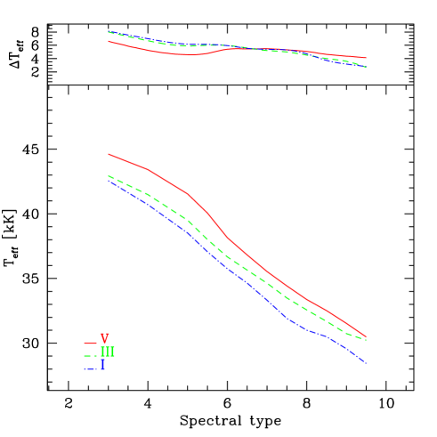
Figure 3: Lower panel: “theoretical” effective temperature scale for dwarfs (solid line), giants (dashed line) and supergiants (dot-dashed line) as derived from our model grid. Upper panel: difference between the $T_{\mathrm{eff}}$ scales of Vacca et al. (vacca (1996)) and the present results.

4.2.2 “Observational” $T_{\mathrm{eff}}$ scale from a sample of Galactic O stars

Instead of relying on a grid of models, one can simply derive mean $T_{\mathrm{eff}}$ scales from the results of detailed spectroscopic analysis of O stars (see also Repolust et al. repolust (2004)). The advantage is that the parameters of the best models are hopefully the true stellar and wind parameters of the stars analysed. But the problem is that the number of objects is limited and that all spectral types are not available (this is especially true for giants). In Figs. 4, 5 and 6, we show the results of a linear regression to the data points (dashed line) in comparison to the $T_{\mathrm{eff}}$ scale derived from the grid of models (solid line).

The linear fits to the observed data are:

$$T_{\rm eff}\ =\left\{\begin{array}[]{l}50838-1995\times\textrm{ST \hskip 28.45274pt (V)}\\ 50882-2115\times\textrm{ST \hskip 28.45274pt (III)}\\ 47666-1881\times\textrm{ST \hskip 28.45274pt (I)}\end{array}\right.$$ (2)

and the dispersions are 1021, 529 and 1446 K respectively.

The differences with the relations of Vacca et al. (vacca (1996)) are also shown in the upper panels of the figures and are slightly smaller (2000 K) than for the theoretical scale, mainly for late spectral types.

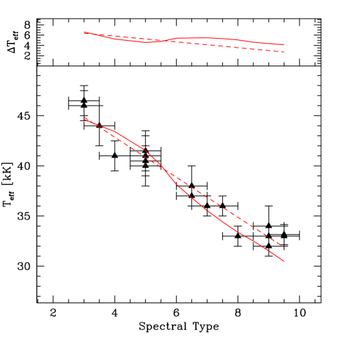
Figure 4: Effective temperature scale for dwarfs as derived from our model grid (“theoretical” scale, solid line) compared to “observational” results based on non-LTE line blanketed models including winds (Herrero et al. hpn02 (2002), Repolust et al. repolust (2004) and Martins et al. wwgal (2005)). The dashed line is the result of linear regression to the data points. The typical error bars for the observational results are $\pm 0.5$ unit for spectral types and are taken from detailed spectroscopic analysis for $T_{\mathrm{eff}}$. The upper panel shows the difference between the relation of Vacca et al. (vacca (1996)) and our $T_{\mathrm{eff}}$ scales (solid line: relation from model grid; dashed line: relation from spectroscopic analysis).

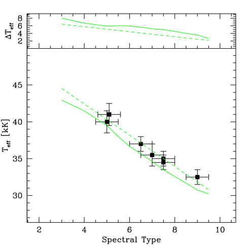
Figure 5: Same as Fig. 4 for giants.

Figure 6: Same as Fig. 4 for supergiants.

4.2.3 Theoretical vs observational $T_{\mathrm{eff}}$ scale

At this point, it is worth discussing the differences between the “theoretical” and the “observational” relation. First of all, given the uncertainties and the natural dispersion of the observational results ($\sim$ 2000-3000 K) the agreement between our theoretical and observational scales is good for dwarfs and supergiants, although our effective temperatures seem to be slightly underestimated (by $\sim$ 1000-2000 K) for late spectral types in our models. For giants, our theoretical $T_{\mathrm{eff}}$ scale seems to be a little too cool (by $\sim$ 1500 K). Note, however, that the number of giants studied so far is relatively small (7).

The following assumptions could be at the origin of the lower effective temperatures in our models compared to the results from the analysis of individual O stars: 1) incorrect metallicity/abundances, 2) incorrect atmosphere and wind parameters (microturbulent velocities, mass loss rates, slope of the wind velocity law), or 3) incorrect gravities. We now discuss these one by one.

1) Metallicity/abundances: First, it is well established that line-blanketing leads to lower $T_{\mathrm{eff}}$ so that a too strong decrease could be due to a too high metal content. However, all stars used for the comparison are Galactic stars which should have solar composition. Of course there is a metallicity gradient in the Galaxy, but the metal content remains within approximately $\pm$ 2 times the solar content (e.g. Giveon et al. 2002a ). Since we have shown that increasing the effective temperature by 1000 to 2000 K required a decrease of the metal content by a factor of 8 (paper I and Martins 2004b ), it is not likely that the difference between our new $T_{\mathrm{eff}}$ scales and observational results can be explained by different metal contents.

2) Atmosphere and wind parameters: Another possibility is that some atmospheric and wind parameters used for our modelling of O stars atmosphere are not exactly the same as the parameters of real O stars. In paper I, we have tested a number of such parameters (microturbulent velocity, mass loss rates, slope of the velocity field in the wind -$\beta$ parameter-) and shown that increasing $v_{\rm turb}$, decreasing $\beta$ or decreasing $\dot{M}$ could lead to later spectral types for a given $T_{\mathrm{eff}}$ (or equivalently to higher $T_{\mathrm{eff}}$ for a given spectral type). Since $\beta$ = 0.8 is already small in our models, it is not likely that this parameter can explain the difference. However, mass loss can explain the discrepancy since most of the late type observed dwarfs in Fig 4 are from Martins et al. (wwgal (2005)) and have $\dot{M}$ much lower than the predictions of the Vink et al. (vink01 (2001)) cooking recipe used to assign a mass loss rates in the present models. Indeed, Martins et al. (wwgal (2005)) found that dwarfs with luminosities below $\sim 10^{5.2}$ L_⊙ have lower mass rates than the results of hydrodynamical simulations. But Fig. 4 shows that the discrepancy between our derived effective temperatures and the observed ones starts for stars with spectral types later than O6, and it turns out that according to our new calibrations an O6V star has a luminosity of $\sim$ 10^5.3 L_⊙. We have also shown in paper I that increasing $\dot{M}$ by a factor 2 lead to a decrease of $\log W^{\prime}$ by $\sim$ 0.1 dex. Hence, it is likely that mass loss is at the origin of the underestimation of $T_{\mathrm{eff}}$ in our models of late type dwarfs compared to results of spectroscopic analysis. Concerning supergiants, the situation is a little more complicated since according to Table 3 all supergiants have luminosities higher than 10^5.2 L_⊙ and should therefore not have reduced winds. Hence, the reason for the lower $T_{\mathrm{eff}}$ in our models is probably not rooted in the mass loss rates.

Mokiem et al. (mokiem (2004)) have also shown, from the computation of theoretical spectra, that an increase of microturbulent velocity from 5 to 20 km s^-1 translates to a shift towards later spectral types by nearly half a sub-type since both He i and He ii lines are stronger but the former are more affected (cf. paper I), although the effect is usually more important on singlet than on triplet He i lines (see also Smith & Howarth sh98 (1998), Villamariz & Herrero vh00 (2000))). This can partly explain the observed behaviour for supergiants for which microturbulent velocities of 20 km s^-1 are possible. Test computation in our models reveal that increasing $v_{\rm turb}$ by such an amount corresponds to a shift in $\log W^{\prime}$ by $\sim$ 0.15, which is of the order of the width of the range of $W^{\prime}$ values within a spectral type. Note also that in our grid of models, we have used $v_{\rm turb}$ = 20 km s^-1 to compute the atmospheric structure. This may be a little to high for dwarfs, but as already discussed (Sect. 2) test models reveal that this does not lead to an overestimation of the line-blanketing effect (only some particular lines are modified).

3) Gravity: Another possibility to explain the different $T_{\mathrm{eff}}$ - scales is that gravities from spectroscopic analysis may be underestimated. This would lead to lower gravities for a given luminosity class, and consequently to lower effective temperatures. However, if we recompute the $T_{\mathrm{eff}}$ scale with gravities increased by the standard deviations obtained from least square fits of observed data, the corresponding increase in $T_{\mathrm{eff}}$ we find ($\sim$ 1000 K, see Sect. 4.2) is not sufficient to explain the difference with observed effective temperatures. This is especially true for giants for which the theoretical effective temperatures are systematically underestimated by $\sim$ 1500 K. Note however that the small number of giants studied so far may hide the natural spread in the $T_{\mathrm{eff}}$ – spectral type relation we see for dwarfs and supergiants. This may thus artificially increase the difference with our theoretical results.

We also want to mention that we have not included the results of Bianchi & Garcia (bg02 (2002)) and Garcia & Bianchi (gb04 (2004)) in our comparisons since they are based on UV analysis, whereas both the present modelling and the observational results of Repolust et al. (repolust (2004)), Herrero et al. (hpn02 (2002)) and Martins et al. (wwgal (2005)) rely on optical diagnostics. Bianchi & Garcia (bg02 (2002)) and Garcia & Bianchi (gb04 (2004)) found effective temperature much lower (by several thousands K) compared to any optical study. This may be partly due to the dependence of the UV diagnostics on several parameters other than $T_{\mathrm{eff}}$, especially clumping which may significantly alter the ionisation structure in the wind (but not the photosphere) and thus the strength of UV lines and which is not taken into account in their analysis.

We note that the present $T_{\mathrm{eff}}$ scale for O dwarfs is slightly cooler ($\sim$ 500 K) than that of paper I. This is explained first by the lower gravities used here for dwarfs (values of 4.00-4.05 were adopted for $\log g$ in paper I) and second by the different pseudo-hydrostatic structure used: ISA-Wind structures were computed in paper I while TLUSTY structures are used here. The difference is illustrated in Fig. 7 where we see the effect of the photospheric structure on the He classification lines in a model with $T_{\mathrm{eff}}$ = 33300 K. TLUSTY structures, which are more realistic due to a better treatment of line-blanketing, have higher temperature and thus a higher thermal pressure which implies a higher density (through the hydrostatic equilibrium equation). This leads to slightly higher ionisations and then to earlier spectral types. The present results should represent an improvement over paper I.

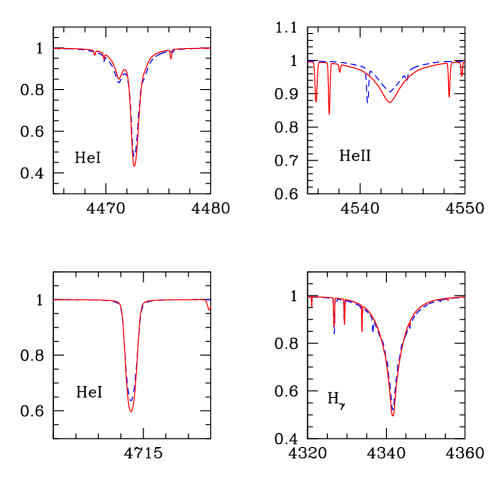
Figure 7: Comparison between H and He line profiles of the same model (A2, see paper I) computed with the Isa-Wind photospheric structure (dashed line) and the TLUSTY structure (solid line). See text for discussion.

The general conclusion of the above discussion is that our theoretical $T_{\mathrm{eff}}$ scale should be taken as indicative and have an uncertainty of $\pm$ 1000 to 2000 K due to both a natural dispersion and uncertainties inherent to our global method. Hence in the following, we use both these theoretical $T_{\mathrm{eff}}$ scales AND the relation derived from detailed modelling of individual stars (“observational” relations) to calibrate the other stellar parameters.

5 Other stellar parameters

We now derive calibrations for the remaining principal stellar parameters based on the two temperature scales determined above. The results are summarised in Tables 1 to 6.

5.1 Magnitudes, bolometric corrections, and luminosities

The calibration of luminosity requires two ingredients: first the absolute visual magnitude and second the bolometric corrections. To calibrate M_V as a function of spectral type, we can either rely entirely on models and proceed exactly as for the effective temperature, i.e. adopting the $\log g$–ST relations, or we can derive empirical calibrations of M_V from results of analysis of individual stars, as we have done for $\log g$. Here, we have chosen the latter method. The advantage is that the derived M_V–ST calibration depends directly on observations and relies less on atmosphere models. It may however suffer from the often poorly know distances of the analysed stars, rendering more uncertain the absolute magnitudes. The former method ($\log g$–ST + M_V from models) relies on better M_V but suffers from the uncertainty in the $\log g$–ST calibration. As the final goal is to produce calibrations as close as possible to observations, we do not retain this method.

The result of the empirical calibration M_V–ST is shown in Fig. 8 where the symbols and observational data are the same as in Fig. 2. The standard deviation is 0.40 for dwarfs, 0.26 for giants and 0.45 for supergiants. The linear fits to the observational data are:

$$M_{V}=\left\{\begin{array}[]{l}0.291\times\textrm{ST - 6.667 \hskip 28.45274pt (V)}\\ 0.147\times\textrm{ST - 6.570 \hskip 28.45274pt (III)}\\ 0.011\times\textrm{ST - 6.388 \hskip 28.45274pt (I)}\end{array}\right.$$ (3)

where $ST$ is the spectral type. One may argue that due to the fact that massive stars evolve almost horizontally in the HR diagram after the main sequence, there could be a wide range of luminosities (and M_V) for a given $T_{\mathrm{eff}}$ (or equivalently ST) for supergiants so that a calibration M_V – ST for luminosity class I stars may be questionable. However, the observed dispersion observed in the present study and in the Vacca et al. (vacca (1996)) study is not significantly different between dwarfs, giants and supergiants. Also, the observed samples show a clear separation in M_V between the different luminosity classes which is even more highlighted by the fact that we consider only 3 luminosity classes (and not 5 as usual). Hence, we think that a calibration M_V – ST even for supergiants makes sense.

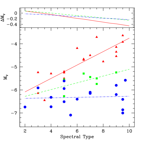
Figure 8: Same as Fig. 2 for absolute magnitudes. The standard deviation from the mean relation is 0.4 mag for dwarfs, 0.26 mag for giants and 0.45 mag for supergiants.

Absolute visual magnitudes have also been derived from observational results by a number of authors. The upper panel of Fig. 8 shows the difference between the calibrations of Vacca et al. (vacca (1996)) and the present ones. They do not differ by more than 0.4 dex which is also the typical dispersion of our relations. Hence, we can not quantitatively compare both types of relations: agreement or small differences ($<$ 0.4 dex) can not be distinguished.

Recently, Schr$\ddot{\rm o}$der et al. (schroder04 (2004)) have tested the M_V–ST relations of Schmidt-Kaler (sk82 (1982)), Howarth & Prinja (hp89 (1989)) and Vacca et al. (vacca (1996)) by comparing the parallaxes derived from such relations to the parallaxes measured by Hipparcos for a number of Galactic O stars. They concluded that the three calibrations are consistent with the Hipparcos measurement. As our relations are not strongly different from the relations of Vacca et al. (vacca (1996)) tested by Schr$\ddot{\rm o}$der et al. (schroder04 (2004)), they are certainly reasonable.

Figure 9: Bolometric correction as a function of effective temperature from our set of CMFGEN models. The solid line is the linear regression (Eq. 4) and the dotted line is the relation of Vacca et al. (vacca (1996)) and is shifted by $\sim$ 0.1 mag compared to our relation.

To obtain the luminosities from absolute magnitudes, one needs to know the bolometric correction. Vacca et al. (vacca (1996)) have shown that bolometric corrections were essentially independent on the luminosity class and depended mainly on $T_{\mathrm{eff}}$. We have computed the BC of our models from luminosities and synthetic M_V, yielding the following linear dependence on $T_{\mathrm{eff}}$:

$$BC=27.58-6.80\times\log T_{\rm eff}$$ (4)

with a standard deviation of 0.05. Our relation is shifted by 0.1 magnitude compared to that of Vacca et al. (vacca (1996)) as seen on Fig. 9. This is explained by the effect of line-blanketing which redistributes the flux blocked at short wavelengths to longer wavelengths, including the optical. This translates to an increase of the V magnitude by $\sim$ 0.1 mag, and consequently to a reduction of the bolometric correction by the same amount (for a model of given luminosity).

Figure 10 shows our calibration of bolometric corrections as a function of spectral type obtained with our theoretical $T_{\mathrm{eff}}$ scale together with the relations of Vacca et al. (vacca (1996)). The difference between both types of relations is displayed in the upper panel. The reduction of BC goes from $\sim$ 0.4 to $\sim$ 0.5 magnitude for dwarfs, from $\sim$ 0.35 to $\sim$ 0.6 mag for giants and from $\sim$ 0.4 to $\sim$ 0.65 mag for supergiants. Figure 11 shows the bolometric corrections estimated with both the “theoretical” and “observational” $T_{\mathrm{eff}}$ scales. Both types of BCs differ by less than 0.2 magnitudes (which is lower than the difference with the results of Vacca et al. vacca (1996)), except for the latest supergiants. The lower BCs at late spectral types for the theoretical relation simply comes from the lower effective temperatures given by the theoretical $T_{\mathrm{eff}}$ scales.

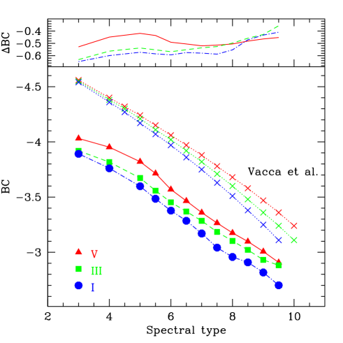
Figure 10: Bolometric correction as a function of spectral type from our set of CMFGEN models (solid lines) and from Vacca et al. (vacca (1996), dotted lines). BCs are usually reduced by $\sim$ 0.2 to 0.5 magnitudes for a given spectral type, the reduction being the largest for early supergiants.

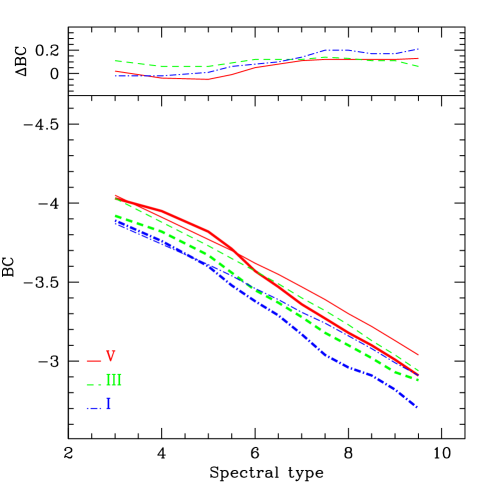
Figure 11: Same as Fig. 10 but with the bolometric corrections derived using the “theoretical” (bold lines) and “observational” (thin lines) $T_{\mathrm{eff}}$ scales. The upper panel shows the differences between “theoretical” and “observational” BCs.

With the absolute magnitudes and bolometric corrections, the luminosities can be estimated according to

$$\log\frac{L}{L_{\odot}}=-0.4\times(M_{\rm{V}}\ +BC-M^{bol}_{\odot})$$ (5)

where $M^{bol}_{\odot}$ is the solar bolometric luminosity taken to be 4.75 (Allen allen (1976)). Again, both theoretical and observational $T_{\mathrm{eff}}$ scales can be used. To estimate the error on the luminosities, we have recomputed them adding $\pm\sigma$ on $\log g$ and M_V in the $\log g$–ST and M_V–ST relations for a given $T_{\mathrm{eff}}$ scale. This means that these errors do not take into account the uncertainty on the effective temperatures. This results in errors of $\pm 0.15,0.10$ and $0.17$ in $\log\frac{L}{L_{\odot}}$ for dwarfs, giants and supergiants respectively. Figure 12 shows the resulting average positions of dwarfs, giants and supergiants in the HR diagram. For a given spectral type, the luminosities are lower by 0.25-0.35 for dwarfs, by $\sim$ 0.25 dex for giants and by 0.25 to 0.35 dex for supergiants compared to the values presented by Vacca et al. (vacca (1996)). Given the small differences in BC for the two $T_{\mathrm{eff}}$ scales it is clear that $L$ depends little on this choice. Quantitatively, using the theoretical or observational $T_{\mathrm{eff}}$ scales results in modifications of the luminosity by less than 0.1 dex for all LC.

A comment concerning the off-set of the dwarfs position compared to the Zero Age Main Sequence seen in Fig. 12 is worthwhile. As we are determining the average properties of O stars, it is not surprising that the O dwarfs relation does not fall on the Zero Age Main Sequence (ZAMS). However, a precise explanation of the offset, indicating average ages of $\sim$ 1 to 5 Myr for early to late O dwarfs, is still lacking. A possible explanation could be that very young stars still embedded in their parental cloud may not be observable. As later types have weaker winds less efficient to blow this cloud, this could possibly even explain why later O dwarfs have older average ages. However, although few, some O dwarfs are found very close to the ZAMS (Rauw gregor (2004), Martins et al. wwgal (2005)). Systematic studies of larger samples of the youngest O stars will be needed to settle this question. Finally, the existence of a theoretical ZAMS is not fully established (Bernasconi & Maeder bm96 (1996)) and the precise shape/location of the ZAMS and isochrones is also dependent on parameters like the rotation rate (Meynet & Maeder mm00 (2000)).

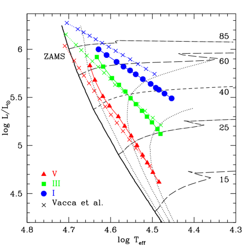
Figure 12: HR diagram showing the typical position of dwarfs (triangles), giants (squares) and supergiants (circles) from the present “theoretical” calibration of $T_{\mathrm{eff}}$ and $\log\frac{L}{L_{\odot}}$. Isochrones for 0, 1, 3 and 5 Myrs are shown together with evolutionary tracks for different masses (taken from Meynet et al. meynet94 (1994)). The crosses and dotted lines are the positions of dwarfs, giants and supergiants following the Vacca et al. (vacca (1996)) calibrations.

5.2 Mass and radius

With the effective temperature scale and the luminosities as a function of spectral type, it is easy to derive the relation radius – spectral type from

$$R=\sqrt{\frac{L}{4\pi\sigma_{R}T_{\rm eff}^{4}}},$$ (6)

where $\sigma_{R}$ is the Stefan-Boltzmann constant. The standard deviation on $R$ is 10 to 20 %.

Gravity can then be used to derive the spectroscopic mass according to

$$M=\frac{gR^{2}}{G},$$ (7)

with $G$ the gravitational constant. Masses must be taken with care since their uncertainty is as high as 35 to 50 %.

For all results see Tables 1 to 6.

5.3 Ionising fluxes

5.3.1 Calibrations

An important quantity related to massive stars is the number of ionising photons they emit due to their high effective temperature and luminosity. Ionising fluxes are defined as follows

$$q_{i}=\int^{\lambda_{i}}_{0}\frac{\pi\lambda F_{\lambda}}{hc}d\lambda$$ (8)

where $F_{\lambda}$ is the flux expressed in erg/s/cm²/Å and $\lambda_{i}$ is the limiting wavelength below which we estimate the ionising flux. In practice, we usually define $q_{0}$, $q_{1}$ and $q_{2}$ as the fluxes able to ionise Hydrogen ($\lambda_{0}$ = 912 Å), He i ($\lambda_{1}$ = 504 Å) and He ii ($\lambda_{2}$ = 228 Å). The ionising fluxes are highly sensitive to line-blanketing effects since metals have most of their bound-free transitions in the Lyman continuum. Hence, the presence of such bound-free opacities in metals modifies the spectral energy distribution (SED) and consequently the ionising fluxes: flux at high energy is blocked and must be re-emitted at longer wavelength. Moreover, the numerous metallic lines in this range create a veil which can also significantly alter the shape of the SED.

Several studies have already provided new ionising fluxes as a function of effective temperature (Smith et al. smith (2002), Mokiem et al. mokiem (2004)). An in depth study of ionising fluxes as a function of spectral type and metallicity (and thus line-blanketing) was carried out by Kudritzki (kud02 (2002)) who found that the number of Lyman continuum photons was not a strong function of metallicity. This may be surprising at first glance since, as we have already mentioned in Sect. 5.1, flux redistribution takes place at all wavelengths, including $\lambda>912$ Å. However, energy flux and photon flux are not equivalent. It is possible for the flux in the Lyman continuum to go down while the photon flux stays almost constant. In this case, most of the photons reside close to the Lyman edge while energy is redistributed at all wavelengths, including $\lambda>912$ Å.

In the studies mentioned above, ionising fluxes where calibrated as a function of effective temperature but not as a function of spectral type. Due to the cooler new effective temperature scales, such calibrations must be significantly different from previous relations based on unblanketed models. For astrophysical applications, the interesting quantity is in fact $Q_{i}$, the total number of ionising photons emitted per unit time related to $q_{i}$ by

$$Q_{i}=q_{i}\times 4\pi R^{2},$$ (9)

with $R$ the stellar radius. With our calibrations $T_{\mathrm{eff}}$–ST and R–ST, we are now able to derive relations between spectral types and the total ionising fluxes $Q_{i}$. However, we have not considered the He ii ionising fluxes since they may be strongly affected by processes not included in our models (shocks, X-rays).

First, we have to calibrate $q_{i}$. For that, we have proceeded as follows: we have built the function $q_{i}(T_{\rm eff},\log g)$ using the same 2D interpolation method as for $T_{\mathrm{eff}}$ (see Sect. 4.2.1) and then we have used the effective temperatures and gravities (relations $T_{\mathrm{eff}}$–ST and $\log g$–ST) for each luminosity class to derive the ionising fluxes of dwarfs, giants and supergiants. Once again, we have used both theoretical and observational $T_{\mathrm{eff}}$ scales to investigate the effects of such relations on the final values of $q_{i}$ (see Tables 1 to 6). Once obtained, these relations have been used with the relations R–ST to derive the calibration $Q_{i}$–spectral type. The results using the theoretical $T_{\mathrm{eff}}$ scale are displayed in Fig. 13. Figure 14 and 15 show the theoretical and observational $Q_{0}$’s and $Q_{1}$’s and the differences between them. Although for Lyman fluxes the differences remain relatively small (lower than 0.3 dex), using different $T_{\mathrm{eff}}$ scales can have a deep impact on the He i ionising fluxes, especially for late type supergiants for which $Q_{1}$ may be changed by a factor 6!

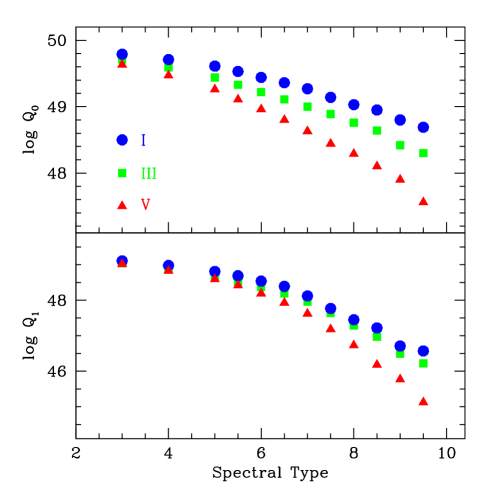
Figure 13: Ionising fluxes as a function of spectral type for dwarfs (triangles), giants (squares) and supergiants (circles) derived using the theoretical $T_{\mathrm{eff}}$ scale.

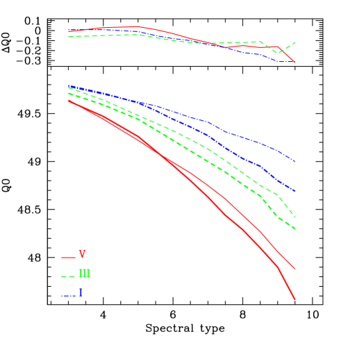
Figure 14: Lyman continuum photon fluxes derived using the theoretical (bold lines) and observational (thin lines) $T_{\mathrm{eff}}$ scales. Solid lines are for dwarfs, dashed lines for giants and dot-dashed lines for supergiants. The upper panel shows the difference between theoretical and observational results.

Figure 15: Same as Fig. 14 but for He i ionising fluxes.

5.3.2 Comparisons with previous predictions

Due to the presence of metals in the model atmospheres, ionising fluxes of O stars are modified: new bound-free opacities increase the blocking of flux at short wavelengths and the numerous metallic lines change the very shape of the spectral energy distribution.

Giveon et al. (2002b ) and Morisset et al. (msbm04 (2004)) have shown that the new generation of atmosphere models including a non-LTE approach, winds and line-blanketing produced more accurate ionising fluxes compared to other previous less sophisticated models. They used the new SEDs to compute photoionisation models and to build excitation diagrams (defined by the ratio of mid-IR nebular lines of Ne, Ar and S). The direct comparison of such diagrams with observations of compact H ii regions with ISO showed the improvement of the new generation models.

Figure 16: Comparison between CMFGEN, TLUSTY and WM-BASIC ionising fluxes for dwarfs. TLUSTY models are from Lanz & Hubeny (ostar2002 (2002)) and WM-BASIC models from Smith et al. (smith (2002)). Note that the latter have been estimated from the original SEDs and not from the SEDs re-binned for the inclusion in Starburst99. The CMFGEN fluxes are taken from Tables 1 to 6.

Figure 17: Same as Fig. 16 for supergiants.

Smith et al. (smith (2002)) computed new ionisation fluxes for O stars using WM-BASIC (Pauldrach et al. wmbasic01 (2001)). Lanz & Hubeny (ostar2002 (2002)) built a grid of plane parallel line-blanketed non-LTE models with TLUSTY and provided H and HeI ionising fluxes. Figures 16 and 17 show the comparison between our ionising fluxes as a function of $T_{\mathrm{eff}}$ for dwarfs and supergiants with those of Smith et al. (smith (2002)) and the TLUSTY grid. Concerning H ionising fluxes, one notes that CMFGEN and TLUSTY agree very well (within 0.1 dex). WM-BASIC models also show similar fluxes for supergiants and for the hottest dwarfs, while $\log q_{0}$ are slightly lower (up to 0.3 dex) for dwarfs with $T_{\mathrm{eff}}$ $<$ 40000 K. The different gravity between our CMFGEN dwarfs ($\log g\sim 3.9$) and the WM-BASIC dwarfs ($\log g=4.0$) may be partly responsible for this difference. However, since the difference in $\log q_{0}$ are equivalent to a shift in $T_{\mathrm{eff}}$ by less than 2000 K (see Fig. 16), we may speculate that a different treatment of line-blanketing between CMFGEN and WM-BASIC may be the main reason for the discrepancy. Concerning the HeI ionising fluxes, CMFGEN and TLUSTY are also in good agreement, which may be surprising given that TLUSTY models do not include winds. However, the largest wind effects are seen in the HeII continuum (Hillier 1987a , 1987b , Gabler et al. gabler89 (1989), Schaerer & de Koter costar3 (1997)). Again, the WM-BASIC HeI ionising fluxes are lower for cool dwarfs ($\sim$ 0.3 dex) and supergiants ($\sim$ 0.1 dex). This results in softer spectra for WM-BASIC models compared to both CMFGEN and TLUSTY models for late dwarfs and supergiants. The exact reasons for this difference leading to an apparent relative overestimate of line blanketing remain unclear but may be likely attributed to different methods used to treat line-blanketing (opacity sampling versus direct inclusion with super-level). The behaviour of several atmosphere models including CMFGEN, TLUSTY and WM-BASIC have been discussed extensively by Morisset et al. (msbm04 (2004)). In short, the CMFGEN and WM-BASIC models do a reasonable job when compared to observed fine structure line ratios of Galactic H ii regions. However, at present the nebular analysis does not allow to favour CMFGEN or WM-BASIC models. New tailored studies of individual nebulae (following e.g. the steps of Oey et al. oey00 (2000)) using these fully blanketed non-LTE models would be required to provide more strongest tests.

The relations $q_{i}(T_{\rm eff})$ allow a direct comparison of atmosphere models, but the quantities of interest for a number of studies (H ii regions, nebular analysis…) are usually the integrated ionising fluxes $Q_{i}$ calibrated as function of spectral type. Such relations ($Q_{i}$–$ST$) depend not only on the model ingredients, but also on the effective temperature scale and on the R–ST relation. Figures 18, 19 and 20 show how our ionising fluxes – spectral type relations derived using both the theoretical and observational effective temperature scales compare to the previous calibrations of Vacca et al. (vacca (1996)) and Schaerer & de Koter (costar3 (1997), CoStar models).

Depending on which $T_{\mathrm{eff}}$ scale is used, two kinds of conclusions can be drawn. First, the theoretical ionising fluxes are lower than in the previous calibrations. Compared to the results of Vacca et al. (vacca (1996)), our $Q_{0}$’s are 0.20 to 0.80 dex lower for dwarfs, 0.25 to 0.55 lower for giants and 0.30 to 0.55 dex lower for supergiants. For $Q_{1}$, the reduction is 0.1 to 1.6(!) dex for LC V, 0.2 to 0.8 dex for LC III and 0.25 to 0.8 dex for LC I. Such reductions are due to two distinct effects: first, the better treatment of line-blanketing compared to the CoStar models and the inclusion of both metals and winds compared to the results of Vacca et al. (vacca (1996)), which modifies the relations $q_{i}(T_{\rm eff})$; second, new relations $T_{\mathrm{eff}}$–ST and R–ST are used to compute $Q_{i}$. These effects render the CMFGEN spectra softer than the CoStar spectra ($\log Q_{1}/Q_{0}$ lower by $\sim$ 0.2 to 1.0 dex). The Vacca et al. (vacca (1996)) predictions are usually harder than the CMFGEN SEDs, except for the earliest spectral types.

Now if we use the $T_{\mathrm{eff}}$ scales derived from the results of detailed spectroscopic analysis of individual massive stars, the ionising fluxes of stars with spectral types earlier than O6 are basically unchanged compared to the results based on the “theoretical” $T_{\mathrm{eff}}$ scale. For later spectral types the reduction of $Q_{i}$ for a given ST is much weaker, $Q_{0}$ and $Q_{1}$ being essentially similar to the Costar and Vacca et al. (vacca (1996)) results for late supergiants. Quantitatively, the reduction of $Q_{0}$ is 0.25 to 0.50 dex (0.20 to 0.35 dex) for dwarfs (giants and supergiants). $Q_{1}$ is much less reduced with the observational scale (0.15 to 1.0 dex for dwarfs and 0.15 to 0.45 dex for giants) and are in fact similar $-$within 0.23 dex$-$ to the Vacca et al. (vacca (1996)) values for late supergiants.

What do we learn from this? The obvious conclusion is that the choice of the underlying effective temperature scale is important to determine the ionising fluxes for a given spectral type and luminosity class. As mentioned in Sect. 4.2, both the theoretical and observational scales have their advantages and drawbacks. At present, we cannot say that one is more relevant than the other, which leaves us with an uncertainty on the ionising fluxes. However, both types of $T_{\mathrm{eff}}$ - scales are significantly cooler than the ones based on plane-parallel H He models. Besides this, it is also worth noting that ionising fluxes are very sensitive to $T_{\mathrm{eff}}$ (especially at low values) so that the difference we find between calibrations of $Q_{i}$s using different $T_{\mathrm{eff}}$ - scales also puts forward the fact that the natural spread in $T_{\mathrm{eff}}$ for a given spectral type (see Figs. 4 to 6) leads to an uncertainty on $Q_{i}$s. And the error on the spectral type (of the order 0.5 unit) also translates to an error on the ionising fluxes (which amounts to a factor of $\sim$ 2 on $Q_{1}$ for late spectral types). Thus, the present results are an improvement over previous analysis and calibrations, but it should be reminded that they still suffer from uncertainties.

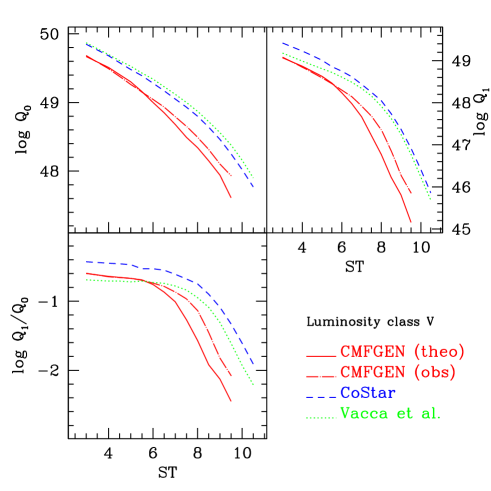
Figure 18: Comparison between the present ionising fluxes of dwarfs and the results of Vacca et al. vacca (1996) and Schaerer & de Koter (costar3 (1997), CoStar models).

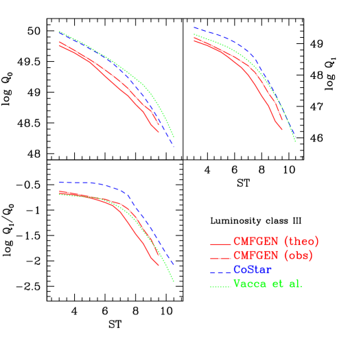
Figure 19: Same as Fig. 18 for giants.

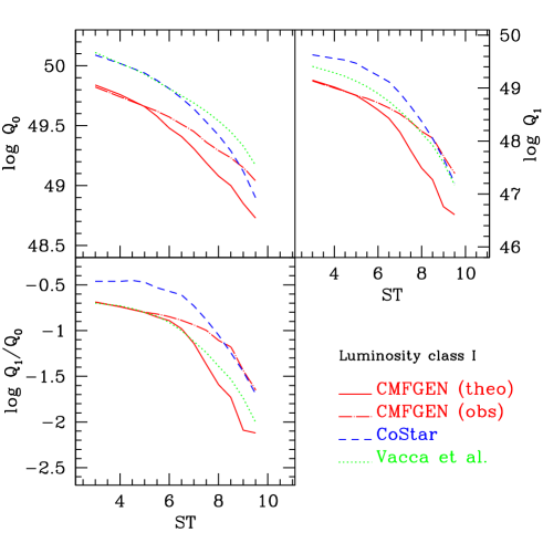
Figure 20: Same as Fig. 18 for supergiants.

Table 1: Stellar parameters as a function of spectral types for luminosity class V stars obtained with the theoretical $T_{\mathrm{eff}}$ scales.

ST	$T_{\mathrm{eff}}$	$\log g_{spec}$	MV	BC	$\log\frac{L}{L_{\odot}}$	R	Mspec	$\log q_{0}$	$\log q_{1}$	$\log Q_{0}$	$\log Q_{1}$
	[K]	[cm s-2]				[R⊙]	[M⊙]	[cm-2 s-1]	[cm-2 s-1]	[s-1]	[s-1]
3	44616	3.92	-5.79	-4.03	5.83	13.84	58.34	24.56	23.96	49.63	49.02
4	43419	3.92	-5.50	-3.95	5.68	12.31	46.16	24.50	23.86	49.47	48.83
5	41540	3.92	-5.21	-3.82	5.51	11.08	37.28	24.38	23.71	49.26	48.59
5.5	40062	3.92	-5.07	-3.71	5.41	10.61	34.17	24.28	23.59	49.11	48.42
6	38151	3.92	-4.92	-3.57	5.30	10.23	31.73	24.15	23.39	48.96	48.19
6.5	36826	3.92	-4.77	-3.47	5.20	9.79	29.02	24.04	23.17	48.80	47.93
7	35531	3.92	-4.63	-3.36	5.10	9.37	26.52	23.91	22.89	48.63	47.62
7.5	34419	3.92	-4.48	-3.27	5.00	8.94	24.15	23.76	22.49	48.44	47.18
8	33383	3.92	-4.34	-3.18	4.90	8.52	21.95	23.65	22.08	48.29	46.73
8.5	32522	3.92	-4.19	-3.10	4.82	8.11	19.82	23.50	21.58	48.10	46.18
9	31524	3.92	-4.05	-3.01	4.72	7.73	18.03	23.34	21.21	47.90	45.77
9.5	30488	3.92	-3.90	-2.91	4.62	7.39	16.46	23.04	20.59	47.56	45.12

Table 2: Same as Table 1 for luminosity class III stars.

ST	$T_{\mathrm{eff}}$	$\log g_{spec}$	MV	BC	$\log\frac{L}{L_{\odot}}$	R	Mspec	$\log q_{0}$	$\log q_{1}$	$\log Q_{0}$	$\log Q_{1}$
	[K]	[cm s-2]				[R⊙]	[M⊙]	[cm-2 s-1]	[cm-2 s-1]	[s-1]	[s-1]
3	42942	3.77	-6.13	-3.92	5.92	16.57	58.62	24.49	23.82	49.71	49.04
4	41486	3.73	-5.98	-3.82	5.82	15.83	48.80	24.41	23.71	49.59	48.89
5	39507	3.69	-5.84	-3.67	5.70	15.26	41.48	24.29	23.53	49.44	48.68
5.5	38003	3.67	-5.76	-3.56	5.63	15.13	38.92	24.19	23.39	49.33	48.53
6	36673	3.65	-5.69	-3.45	5.56	14.97	36.38	24.08	23.23	49.22	48.37
6.5	35644	3.63	-5.62	-3.37	5.49	14.74	33.68	23.99	23.07	49.11	48.19
7	34638	3.61	-5.54	-3.28	5.43	14.51	31.17	23.89	22.85	49.00	47.96
7.5	33487	3.59	-5.47	-3.18	5.36	14.34	29.06	23.79	22.55	48.89	47.64
8	32573	3.57	-5.40	-3.10	5.30	14.11	26.89	23.68	22.21	48.76	47.29
8.5	31689	3.55	-5.32	-3.02	5.24	13.88	24.84	23.57	21.90	48.64	46.97
9	30737	3.53	-5.25	-2.93	5.17	13.69	23.07	23.37	21.43	48.42	46.49
9.5	30231	3.51	-5.18	-2.88	5.12	13.37	21.04	23.27	21.18	48.30	46.22

Table 3: Same as Table 1 for luminosity class I stars.

ST	$T_{\mathrm{eff}}$	$\log g_{spec}$	MV	BC	$\log\frac{L}{L_{\odot}}$	R	Mspec	$\log q_{0}$	$\log q_{1}$	$\log Q_{0}$	$\log Q_{1}$
	[K]	[cm s-2]				[R⊙]	[M⊙]	[cm-2 s-1]	[cm-2 s-1]	[s-1]	[s-1]
3	42551	3.73	-6.35	-3.89	6.00	18.47	66.89	24.47	23.79	49.79	49.11
4	40702	3.65	-6.34	-3.76	5.94	18.91	58.03	24.38	23.64	49.71	48.98
5	38520	3.57	-6.33	-3.60	5.87	19.48	50.87	24.25	23.45	49.61	48.81
5.5	37070	3.52	-6.33	-3.48	5.82	19.92	48.29	24.15	23.31	49.53	48.69
6	35747	3.48	-6.32	-3.38	5.78	20.33	45.78	24.04	23.14	49.44	48.54
6.5	34654	3.44	-6.31	-3.29	5.74	20.68	43.10	23.95	22.97	49.36	48.39
7	33326	3.40	-6.31	-3.17	5.69	21.14	40.91	23.84	22.69	49.27	48.12
7.5	31913	3.36	-6.30	-3.04	5.64	21.69	39.17	23.68	22.32	49.14	47.77
8	31009	3.32	-6.30	-2.96	5.60	22.03	36.77	23.56	21.97	49.03	47.45
8.5	30504	3.28	-6.29	-2.91	5.58	22.20	33.90	23.48	21.75	48.95	47.22
9	29569	3.23	-6.29	-2.82	5.54	22.60	31.95	23.31	21.22	48.80	46.71
9.5	28430	3.19	-6.28	-2.70	5.49	23.11	30.41	23.17	21.05	48.69	46.57

Table 4: Stellar parameters as a function of spectral types for luminosity class V stars obtained with the observational $T_{\mathrm{eff}}$ scales.

ST	$T_{\mathrm{eff}}$	$\log g_{spec}$	MV	BC	$\log\frac{L}{L_{\odot}}$	R	Mspec	$\log q_{0}$	$\log q_{1}$	$\log Q_{0}$	$\log Q_{1}$
	[K]	[cm s-2]				[R⊙]	[M⊙]	[cm-2 s-1]	[cm-2 s-1]	[s-1]	[s-1]
3	44852	3.92	-5.79	-4.05	5.84	13.80	57.95	24.57	23.98	49.64	49.04
4	42857	3.92	-5.50	-3.91	5.67	12.42	46.94	24.47	23.82	49.44	48.79
5	40862	3.92	-5.21	-3.77	5.49	11.20	38.08	24.34	23.66	49.22	48.54
5.5	39865	3.92	-5.07	-3.70	5.41	10.64	34.39	24.27	23.57	49.10	48.41
6	38867	3.92	-4.92	-3.62	5.32	10.11	30.98	24.20	23.46	48.99	48.26
6.5	37870	3.92	-4.77	-3.55	5.23	9.61	28.00	24.13	23.34	48.88	48.09
7	36872	3.92	-4.63	-3.47	5.14	9.15	25.29	24.04	23.17	48.75	47.88
7.5	35874	3.92	-4.48	-3.39	5.05	8.70	22.90	23.94	22.98	48.61	47.64
8	34877	3.92	-4.34	-3.30	4.96	8.29	20.76	23.82	22.68	48.44	47.30
8.5	33879	3.92	-4.19	-3.22	4.86	7.90	18.80	23.69	22.23	48.27	46.81
9	32882	3.92	-4.05	-3.13	4.77	7.53	17.08	23.52	21.69	48.06	46.22
9.5	31884	3.92	-3.90	-3.04	4.68	7.18	15.55	23.39	21.31	47.88	45.80

Table 5: Same as Table 4 for luminosity class III stars.

ST	$T_{\mathrm{eff}}$	$\log g_{spec}$	MV	BC	$\log\frac{L}{L_{\odot}}$	R	Mspec	$\log q_{0}$	$\log q_{1}$	$\log Q_{0}$	$\log Q_{1}$
	[K]	[cm s-2]				[R⊙]	[M⊙]	[cm-2 s-1]	[cm-2 s-1]	[s-1]	[s-1]
3	44537	3.77	-6.13	-4.03	5.96	16.19	55.95	24.57	23.94	49.77	49.14
4	42422	3.73	-5.98	-3.88	5.85	15.61	47.43	24.47	23.78	49.64	48.95
5	40307	3.69	-5.84	-3.73	5.73	15.07	40.43	24.34	23.61	49.48	48.75
5.5	39249	3.67	-5.76	-3.65	5.67	14.82	37.35	24.28	23.51	49.40	48.63
6	38192	3.65	-5.69	-3.57	5.61	14.58	34.53	24.21	23.41	49.32	48.52
6.5	37134	3.63	-5.62	-3.49	5.54	14.36	31.96	24.13	23.28	49.23	48.38
7	36077	3.61	-5.54	-3.40	5.48	14.14	29.59	24.04	23.16	49.13	48.24
7.5	35019	3.59	-5.47	-3.32	5.42	13.93	27.45	23.94	22.96	49.01	48.03
8	33961	3.57	-5.40	-3.23	5.35	13.74	25.49	23.82	22.68	48.88	47.74
8.5	32904	3.55	-5.32	-3.13	5.28	13.55	23.68	23.70	22.32	48.75	47.37
9	31846	3.53	-5.25	-3.04	5.21	13.38	22.04	23.61	22.02	48.65	47.06
9.5	30789	3.51	-5.18	-2.94	5.15	13.22	20.55	23.39	21.50	48.42	46.53

Table 6: Same as Table 4 for luminosity class I stars.

ST	$T_{\mathrm{eff}}$	$\log g_{spec}$	MV	BC	$\log\frac{L}{L_{\odot}}$	R	Mspec	$\log q_{0}$	$\log q_{1}$	$\log Q_{0}$	$\log Q_{1}$
	[K]	[cm s-2]				[R⊙]	[M⊙]	[cm-2 s-1]	[cm-2 s-1]	[s-1]	[s-1]
3	42233	3.73	-6.35	-3.87	5.99	18.56	67.53	24.46	23.77	49.78	49.09
4	40422	3.65	-6.34	-3.74	5.93	18.99	58.54	24.36	23.62	49.70	48.96
5	38612	3.57	-6.33	-3.61	5.87	19.45	50.72	24.25	23.46	49.62	48.82
5.5	37706	3.52	-6.33	-3.54	5.84	19.70	47.25	24.20	23.38	49.58	48.76
6	36801	3.48	-6.32	-3.46	5.81	19.95	44.10	24.14	23.29	49.52	48.67
6.5	35895	3.44	-6.31	-3.39	5.78	20.22	41.20	24.07	23.18	49.46	48.58
7	34990	3.40	-6.31	-3.31	5.75	20.49	38.44	24.00	23.06	49.41	48.47
7.5	34084	3.36	-6.30	-3.24	5.72	20.79	36.00	23.89	22.89	49.31	48.31
8	33179	3.32	-6.30	-3.16	5.68	21.10	33.72	23.81	22.70	49.25	48.14
8.5	32274	3.28	-6.29	-3.08	5.65	21.41	31.54	23.74	22.56	49.19	48.00
9	31368	3.23	-6.29	-2.99	5.61	21.76	29.63	23.65	22.21	49.11	47.67
9.5	30463	3.19x	-6.28	-2.91	5.57	22.11	27.83	23.52	21.87	49.00	47.35

6 Discussion: metallicity effects

The present study is restricted to the case of a solar metallicity for atmosphere models. First, we want to highlight that we have used a solar composition for all luminosity classes. This assumption is certainly good for dwarfs, but may be too crude for supergiants which usually show hints of He enrichment and modified CNO abundances (e.g. Herrero et al. her92 (1992), Walborn et al. walborn04 (2004)). These changes are likely different from star to star since they depend on rotational velocities (Meynet & Maeder mm00 (2000)). Hence, non solar He abundance may slightly affect the strength of the classification lines and introduce a dispersion in ST for a given $T_{\mathrm{eff}}$. Also, although Iron dominates the blanketing effect in terms of lines, CNO elements are important for the blocking of radiation through their bound-free transitions usually close to the He II edge so that, although the sum of C, N and O abundances are constant during CNO processing, a change in the abundance of each element may modify the global blanketing effect. Such an effect should be further studied by new analyses of supergiants. Second, the present work does not address the important question of the dependence of the fundamental parameters of O stars on global metallicity. Nonetheless, several indications of the general trend exist.

From the modelling side, Kudritzki kud02 (2002) and Mokiem et al. (mokiem (2004)) have investigated the effect of a change of the metal content on the spectral energy distribution of O dwarfs using CMFGEN models. They found that H ionising fluxes are essentially unchanged when Z is varied between twice and one tenth the solar content. They argue that the redistribution of the flux blocked by metals at short wavelengths takes place within the Lyman continuum, which explains the observed behaviour. However, they show that the SEDs are strongly modified below $\sim$ 450 Å, spectra being softer at higher metallicity (see also Sect. 5.3.1). Morisset et al. (msbm04 (2004)) have computed various WM-BASIC models at different metallicities and showed how Z affected the strength of mid-IR nebular lines emitted in compact H ii regions. The softening of the SEDs when metallicity increases is crucial to understand the behaviour of observed excitations sequences.

Concerning the effect of metallicity on $T_{\mathrm{eff}}$ scales, Mokiem et al. (mokiem (2004)) have shown that for a given $T_{\mathrm{eff}}$, spectral types vary within one subclass when Z is decreased from 2 to 0.1 $Z_{\odot}$. This boils down to a higher effective temperature at low metallicity than at solar metallicity. We reach the same conclusion from the study of several test models for dwarfs with Z = 1/8 $Z_{\odot}$ (see Martins 2004b ). We estimate that the reduction of the $T_{\mathrm{eff}}$ scale (compared to pure H He results) at this metallicity is roughly half the reduction obtained at solar metallicity (see also Martins et al. teffscale (2002)).

Observationally, Massey et al. (massey04 (2004)) derived effective temperatures of a sample of O stars in the Magellanic Clouds by means of models computed with the code FASTWIND (Santolaya-Rey et al. fast97 (1997)). They found lower $T_{\mathrm{eff}}$ than Vacca et al. (vacca (1996)) but higher than those of Galactic O stars, in good agreement with our results. They estimate that effective temperatures of early to mid O type MC objects are 3000 to 4000 K hotter than Galactic counterparts. Previously, Crowther et al. (paul02 (2002)) computed CMFGEN models and showed that extreme O supergiants in the Magellanic Clouds were cooler by 5000 to 7500 K compared to the Vacca et al. (vacca (1996)) calibration. Bouret et al. (jc03 (2003)) also confirmed the reduction of effective temperatures in SMC O dwarfs using CMFGEN models. However, they derived temperatures in agreement our $T_{\mathrm{eff}}$ scale for Galactic stars, which may be surprising given the lower metallicity of the SMC. Even more recently, Heap et al. (heap05 (2005)) submitted a paper in which they derive the stellar properties of a large sample of SMC stars. Again, the effective temperatures are not inconsistent with those of Galactic stars. They also provide bolometric corrections and ionising fluxes which are in better agreement with our new calibration than with the older pure H He plane-parallel ones. Given the dispersion in the data points, a conclusion as regards the metallicity dependence is not possible.

The above discussion shows that although hints on the metallicity dependence of stellar parameters of O stars exists, a quantitative and systematic study remains to be carried out.

7 Concluding remarks

We have presented new calibrations of stellar parameters of O stars as a function of spectral type based on atmosphere models computed with the code CMFGEN (Hillier & Miller hm98 (1998)). We have build a grid of models spanning the range of spectral types and luminosity classes of O stars from which calibrations have been derived through 2D interpolations. The main improvement of such relations over previous ones is the inclusion of line-blanketing and winds in the non-LTE atmosphere models. Our main results are the following:

• We have derived two types of effective temperature scales: a theoretical one based uniquely on our grid of models (approach similar to paper I) and an observational one from the results of detailed spectroscopic analysis of individual O stars with line blanketed non-LTE models including winds. We confirm the now well established fact that line-blanketing leads to cooler effective temperature scales compared to the widely used relations of Vacca et al. (vacca (1996)) based on plane-parallel pure H He models. The adoption of a better photospheric structure in our models leads to slightly cooler ($\sim$ 500 K) theoretical effective temperatures compared to our first results (Martins et al. teffscale (2002)). Our theoretical $T_{\mathrm{eff}}$–ST relations are cooler by 2000 to 8000 K — being larger for earlier spectral types and lower luminosity classes — compared to Vacca et al. (vacca (1996)) calibrations. The theoretical $T_{\mathrm{eff}}$ scales are consistent with observational relations for early type dwarfs and supergiants and are slightly cooler for late type spectral types (by up to 2000 K for supergiants). This may be due to too high mass loss rates in our models. For giants, the theoretical relation is systematically cooler by $\sim$ 1000 K. We estimate the uncertainty of our theoretical effective temperatures to be between 1000 and 2000 K for a given spectral type. This is due to the intrinsic dispersion of temperatures for O stars of a given spectral type and to the uncertainties of the models (hydrodynamic structure, adopted parameters).

• Bolometric corrections are reduced compared to the calibrations of Vacca et al. (vacca (1996)), the reduction being larger for supergiants and for the earliest spectral types. BC’s estimated using the theoretical $T_{\mathrm{eff}}$ scales are 0.40 to 0.50 (resp. 0.35 to 0.60, 0.40 to 0.65) mag lower for dwarfs (resp. giants, supergiants), while those estimated using the observational relations are 0.30 to 0.50 (resp. 0.30 to 0.50, 0.20 to 0.65) mag lower for luminosity class V (resp. III, I).

• Luminosities are reduced by 0.20 to 0.35 dex for dwarfs, 0.25 dex for giants and 0.25 to 0.35 dex for supergiants compared to the calibrations of Vacca et al. (vacca (1996)) with little difference ($\lesssim$ 0.1 dex) between results using theoretical and observational relations. The reduction of luminosity is independent of spectral type for giants and supergiants and is slightly larger for late type than for early type dwarfs.

• For a given spectral type, ionising fluxes are reduced due to the effect of line-blanketing on the SED (blocking of flux). Compared to the Vacca et al. (vacca (1996)) values and using our theoretical $T_{\mathrm{eff}}$ scale, we find integrated Lyman ionising fluxes ($Q_{0}$) 0.20 to 0.80 dex lower for dwarfs, the larger difference being at late spectral types. The reduction is 0.25 to 0.55 dex (resp. 0.30 to 0.55 dex) for giants (resp. supergiants). If we use the observational effective temperature scale, the reduction are 0.25 to 0.50 dex for dwarfs and 0.20 to 0.35 dex for giants and supergiants. He i ionising fluxes are also reduced, the difference between theoretical and observational results being larger.

  For a given $T_{\mathrm{eff}}$, our $q_{i}$’s agree well with the TLUSTY grid OSTAR2002 (Lanz & Hubeny ostar2002 (2002)), but for late spectral types, they are larger by up to 0.3 dex compared to the results of Smith et al. (smith (2002)) based on WM-BASIC models. This shows that current atmosphere codes are not fully consistent and indicates that the typical uncertainty on current ionising fluxes per unit area may still be up to a factor of $\sim$ 2 for a given effective temperature.

Our results should be tested further when more analysis of individual stars are available and cover the whole range of spectral types and luminosity classes. Despite some remaining uncertainties on the $T_{\mathrm{eff}}$ scale, our results should represent a significant improvement over previous calibrations, given the detailed treatment of non-LTE line-blanketing in the expanding atmospheres of massive stars.

- (1) Abbott, D.C. & Hummer, D.G., 1985, ApJ, 294, 286
- (2) Allen, C.W., 1976, Astrophysical Quantities, (London: Athlone)
- (3) Auer, L.H. & Mihalas, D., 1972, ApJS, 205, 24
- (4) Bernasconi, P.A. & Maeder, A., 1996, A&A, 307, 829
- (5) Bianchi, L. & Garcia, M., 2002, ApJ, 581, 610
- (6) Bouret, J.C., Lanz, T, Hillier, D.J., Heap, S.R., Hubeny, I., Lennon, D.J., Smith, L.J., Evans, C.J., 2003, ApJ, 595, 1182
- (7) Bouret, J.C., Lanz, T., Hillier, D.J., 2005, A&A, in press, astro-ph/0412346
- (8) Conti, P.S., 1973, ApJ, 179, 181
- (9) Crowther, P.A., et al., 2002, ApJ, 579, 774
- (10) Evans, C.J., Crowther, P.A., Fullerton, W., Hillier, D.J., ApJ, 610, 1021
- (11) Gabler,R., Gabler, A., Kudritzki, R.P., Puls, J., Pauldrach, A.W.A., 1989, A&A, 226, 162
- (12) Garcia, M. & Bianchi, L., 2004, ApJ, 606, 497
- (13) Giveon, U., Morisset, C., Sternberg, A., 2002a, A&A, 392, 501
- (14) Giveon, U, Sternberg, A., Lutz, D., Feuchtgruber, H., Pauldrach, A.W.A., 2002b, ApJ, 566, 880
- (15) Grevesse, N. & Sauval, A., 1998, Space Sci. Rev, 85, 161
- (16) Hamann, W.R., 1986, A&A, 160, 347
- (17) Heap, S.R., Lanz, T., Hubeny, I., 2005, ApJ, submitted, astro-ph/0412345
- (18) Herrero, A., Kudritzki, R.P., Vilchez, J.M., Kunze, D., Butler, K., Haser, S., 1992, A&A, 261, 209
- (19) Herrero, A., Puls, J., Villamariz, M.R., 2000, A&A, 354, 193
- (20) Herrero, A., Puls, J., Najarro, F., 2002, A&A, 396, 949
- (21) Hillier, D.J., 1987a, ApJS, 63, 965
- (22) Hillier, D.J., 1987b, ApJS, 63, 987
- (23) Hillier, D.J. & Miller, D.L., 1998, ApJ, 496, 407
- (24) Hillier, D.J., et al., 2003, ApJ, 588, 1039
- (25) Howarth, I.D. & Prinja, R.K., 1989, ApJS, 69, 527
- (26) Hubeny, I. & Lanz, T., 1995, ApJ, 439, 875
- (27) Kudritzki, R.P., 1992, A&A, 266, 395
- (28) Kudritzki, R.P., 1998, in “Stellar Astrophysics for the Local Group”, proc. of the VIIIth Canary Island Winter School, eds. A. Aparacio, A. Herrero, F. Sanchez, p. 149-262
- (29) Kudritzki, R.P. & Puls, J., 2000, ARA&A, 38, 613
- (30) Kudritzki, R.P., 2002, ApJ, 577, 389
- (31) Lamers. H.G.J.L.M., Snow, T.P. & Lindholm, D.M., 1995, ApJ, 455, 269
- (32) Lanz, T. & Hubeny, I., 2002, ApJS, 146, 417
- (33) Markova, N, Puls, J., Repolust, T., Markov, H., 2004, A&A, 413, 693
- (34) Martins, F., Schaerer, D., Hillier, D.J., 2002, A&A, 382, 999. paper I
- (35) Martins, F., Schaerer, D., Hillier, D.J., Heydari-Malayeri, M., 2004, A&A, 420, 1087
- (36) Martins, F., 2004b, PhD thesis, Université Paul Sabatier, Toulouse, France
- (37) Martins, F., Schaerer, D., Hillier, D.J., Meynadier, F., Heydari-Malayeri, M., 2005, A&A, submitted
- (38) Massey, P., Bresolin, F., Kudritzki, R.P., Puls, J., Pauldrach, A.W.A., 2004, ApJ, 608, 1001
- (39) Mathys, G., 1988, A&AS, 76, 427
- (40) Meynet, G., Maeder, A., Schaller, G., Schaerer, D., Charbonnel, C., 1994, A&AS, 103, 97
- (41) Meynet, G. & Maeder, A., 2000, A&A, 361, 101
- (42) Mokiem, M.R., Martín-Hernández, N.L., Lenorzer, A., de Koter, A., Tielens, A.G.G.M., A&A, 419, 319
- (43) Morisset, C., Schaerer, D., Bouret, J.C., Martins, F., 2004, A&A, 415, 577
- (44) Najarro, F., Kudritzki, R.P., Cassinelli, J.P., Stahl, O., Hillier, D.J., 1996, A&A, 306, 892
- (45) Pauldrach, A.W.A., Hoffmann, T.L., Lennon, M., 2001, A&A, 375, 161
- (46) Oey, M.S., Dopita, M.A., Shields, J.C., Smith, R.C., 2000, ApJ, 128, 511
- (47) Puls, J., Urbaneja, M.A., Venero, R., Repolust, T., Springmann, U., Jokuthy, A., Mokiem, M.R., 2005, A&A, submitted (astro-ph/0411398)
- (48) Rauw, G., 2004, in “Evolution of Massive Stars, Mass Loss and Winds”, Summer School on Stellar Physics, Eds. M. Heydari-Malayeri, Ph. Stee and J.P. Zahn, p. 293
- (49) Repolust, T., Puls, J., Herrero, A., 2003, A&A, 415, 349
- (50) Santolaya-Rey, A.E., Puls, J., Herrero, A., 1997 A&A, 323, 488
- (51) Schaerer, D. & Schmutz, W., 1994, A&A, 1288, 231
- (52) Schaerer, D. & de Koter, A., 1997, A&A, 322, 598
- (53) Schmidt-Kaler, T., 1982, in Landoldt-Brnstein, New Seriesm Group, VI, Vol. 2, eds, K. Schaifers & H.H. Voigt (Berlin: Springer-Verlag), 1
- (54) Schrder, S.E., Kaper, L., Lamers, H.J.G.L.M., Brown, A.G.A., A&A, in press, astro-ph/0408370
- (55) Smith, K.C. & Howarth, I.D., 1998, MNRAS, 299, 1146
- (56) Smith, L.J., Norris, R.P.F., Crowther, P.A., 2002, MNRAS, 337, 1309
- (57) Vacca, W.D., Garmany, C.D., Shull, J.M., 1996, ApJ, 460, 914
- (58) Villamariz, M.R. & Herrero, A., 2000, A&A, 357, 597
- (59) Vink, J., de Koter, A., Lamers, H.J.G.L.M., 2001, A&A, 369, 574
- (60) Walborn, N.R., Morrell, N.I., Howarth, I.D., Crowther, P.A., Lennon, D.J., Massey, P., 2004, ApJ, 608, 1028