Analysis of medium resolution spectra by automated methods - application to M 55 and $\omega$ Centauri

We have employed feedforward neural networks trained on synthetic spectra in the range 3800 to 5600 Å with resolutions of $\sim$ 2-3 Å to determine metallicities from spectra of about 1000 main-sequence turn-off, subgiant and red giant stars in the globular clusters M 55 and $\omega$ Cen. The overall metallicity accuracies are of the order of 0.15 to 0.2 dex. In addition, we tested how well the stellar parameters log $g$ and $T_{\rm eff}$ can be retrieved from such data without additional colour or photometric information. We find overall uncertainties of 0.3 to 0.4 dex for log $g$ and 140 to 190 K for $T_{\rm eff}$. In order to obtain some measure of uncertainty for the determined values of [Fe/H], log $g$ and $T_{\rm eff}$, we applied the bootstrap method for the first time to neural networks for this kind of parametrization problem. The distribution of metallicities for stars in $\omega$ Cen clearly shows a large spread in agreement with the well known multiple stellar populations in this cluster.

1 Introduction

The advance in modern spectroscopic techniques coupled with 8-meter class telescopes makes it possible to simultaneously obtain spectra for a large number of stars in clusters. Although such spectra as analysed in this work do not have high enough resolution to make detailed line analyses, they offer the possibility to measure abundances with good precision ($\sim$ 0.2 dex). This permits, for example, statistically significant analyses of stellar populations in dwarf spheroidal galaxies or studies of the intra- and intercluster abundance variations of globular clusters.

While the data acquisition and subsequent reduction are themselves challenging, the analysis of such a large amount of data can be efficiently handled by the introduction of automated methods. This can be as accurate as spectral analyses (using line indices etc.) carried out by a human expert, as proven in several earlier works (see e.g. Snider et al. 2001, Soubiran et al. 1998). Several of these works show that the accuracy of the results was limited by the quality of the data rather than by the automated algorithm used to analyse them.

Figure 1: Examples of observed spectra. The left panels show the spectra as obtained by the blue grism, the right column that of the red grism. The upper panel shows spectra of a red giant star, the lower for a main sequence star in M 55, i.e. [Fe/H] = $-$1.8 dex. Note the larger number of absorption lines in the spectrum of the cool giant. In the lower plot the wavelength ranges used for the neural network analysis are indicated.

Recent studies using automated methods to retrieve stellar parameters $T_{\rm eff}$, log $g$ and [Fe/H] from observed data were limited in various ways. (In the following we call this process ‘parametrization’.) For example, Bonifacio & Caffau (2003) employed a minimum distance-based classifier to high resolution spectra of stars in the Sagittarius Dwarf Spheroidal but were restricted to certain luminosities and temperatures. Earlier efforts, especially those using neural networks, were also limited in their analysis of errors of the determined stellar parameters. Most often, the precision with which stellar parameters can be retrieved is evaluated by using a validation set with known target values. While this is correct to get some estimate of the overall uncertainty, this technique cannot be applied to previously unseen data, where such additional information is of course not available. However, any parameter estimate is only meaningful if some direct measure of uncertainty can be applied. To overcome this, we employed the bootstrap method to neural networks which allows us to assign individual error bars to the estimated stellar parameters.

Snider et al. (2001), using neural networks on spectral data with resolutions similar to those in this work, could determine all three stellar parameters ($T_{\rm eff}$, log $g$ and [Fe/H]) well. Indeed, they showed that the precisions are similar to those that can be obtained from fine analyses of high resolution spectra. While their neural network training and validation sets contained spectra from spectroscopic observations, our work relies entirely on synthetic spectra as templates. Of course, ‘real world’ spectroscopic data with stellar parameters assigned from spectral synthesis analyses are the ideal case but are expensive in terms of observing time and effort. In this work we demonstrate that synthetic spectra in combination with automated methods can be used to determine reliable stellar parameters from spectroscopic observations.

We examine spectra from stars in the globular clusters M 55 and $\omega$ Centauri. These clusters serve as a demonstration of our methods. We have recently obtained a much larger database of stellar spectra in several globular clusters, and these will be subject to an extensive analysis in the future. M 55 has a metallicity of about $-$1.80 dex (Zinn & West 1984, Harris 1996, Richter et al. 1999) and is used primarily to validate our method. $\omega$ Cen, in contrast, is known to harbour several stellar populations with different kinematical characteristics and a metallicity range from $-$2.5 to $-$0.5 dex (see e.g Norris & Da Costa 1995, Suntzeff & Kraft 1996), suggesting an entirely different formation history to that of normal globular clusters. Indeed, several earlier spectroscopic and photometric studies found a prolonged formation period of about 2 to 5 Gyr, suggesting that this object is more likely the nucleus of an accreted dwarf galaxy than a globular cluster (Lee et al. 1999, Hilker & Richtler 2000, Hughes et al. 2004, and especially Hilker et al. 2004). In addition, it was found that there is a clear trend of the $\alpha$ element abundances with the overall metallicity (see e.g. Pancino et al. 2002 or Origlia et al. 2003). The populations in $\omega$ Cen can be subdivided into a dominant metal-poor component with a metallicity peak at $-$1.7 dex which accounts for about 70% of the stars. Some 25% of the stars belong to the intermediate metallicity population with [Fe/H] $\sim$ $-$1.2 dex while the last 5% are metal-rich stars with [Fe/H] $\sim$ $-$0.6 dex (see e.g. Smith 2004).

The purpose of this work is to demonstrate the ability of automated methods (here neural networks) to derive accurate metallicities as well as surface temperatures and gravities from spectra with medium resolutions of $\sim$ 2-3 Å. Sect. 2 and 3 give a summary of the acquisition, reduction and selection of the observations, while Sect. 4 describes the set of synthetic spectra. The training procedure of the neural networks and the application of the bootstrap method are described in Sect. 5. In Sect. 6 the networks are validated on (observed) spectra of stars in M 55 (with known metallicity and log $g$ and $T_{\rm eff}$ estimated from isochrones) as well as specific stars with known stellar parameters. The same networks are then applied to stellar spectra in $\omega$ Cen in order to derive preliminary metallicity values. Since this cluster is indeed very peculiar, we do not attempt to interpret these results in great detail. Rather, we want to show that the networks can yield reliable results across a large range of abundances for stars in different evolutionary states.

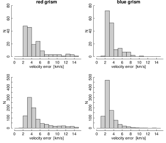
Figure 2: Distributions of the velocity errors of the red grism (left column) and blue grism (right column) for the spectra of M 55 (top panels) and $\omega$ Cen (bottom panels). The errors in the red grism are somewhat larger because of a smaller number of prominent absorption lines available for the cross-correlation procedure.

2 Observations and reductions

2.1 Data acquisition

The data were obtained on the nights 7-12 May 2002 at the VLT at ESO/Paranal (Chile) in visitor mode. The instrument was the FORS2 low dispersion spectrograph in combination with the mask exchange unit (MXU) and a 4 $\times$ 4 k MIT CCD with a field of view of 6.8 square arcminutes. On average, about 60 stars were observed per mask, with the candidates chosen from Strömgren photometry (Hilker & Richtler 2000). The slit width was fixed to 1^′′ and the slit length ranged from 5 to 7^′′. The seeing was always better than 1^′′. While Hilker et al. (2004) and Kayser et al. (2005) examined the main-sequence turn-off and SGB stars, the present work includes observations of the red giant and upper main sequence stars in both $\omega$ Cen and M 55. Each mask was observed through a ‘blue’ grism (ESO 600I+25, second order) and a ‘red’ grism (ESO 1400V+18) with maximum wavelength coverages of 3690 to 4888 Å and 4560 to 5860 Å. The corresponding dispersions are 0.58 Å pix^-1 and 0.62 Å pix^-1, respectively. The exposure times were chosen in such a way as to ensure that the minimum signal to noise ratio (S/N) per pixel was $\sim$ 40–50 for the majority of objects. For giant stars, the average S/N was slightly larger, about $\sim$ 70–80. In the same way, the observations for M 55 were carried out with different masks for main-sequence, subgiant and giant stars. In order to have reference spectra from stars with known stellar parameters, long slit spectra with the same grism/filter combinations were obtained for eleven bright stars with a typical S/N of about 100–150. These stars are referred to as ‘standard stars’ in the following. In addition to the science frames, bias, flat field and wavelength calibration images were obtained during daytime. The log of the observations reduced for this work is shown in Table 1. A summary and outline of the reductions and analysis based on line indices for the main sequence turn-off stars is found in Hilker et al. (2004) and Kayser et al. (2005). It should be noted that the sample of observed stars is not complete. The focus of these observations was to get a large sample of main-sequence turn-off and subgiant stars which are best suited to break the age-metallicity degeneracy. The upper main-sequence and red giant stars primarily serve to provide additional constraints for isochrone fitting of the different (age/metallicity) populations in $\omega$ Cen.

Table 1: Table of the observations reduced and analysed for this work in addition to those reported by Kayser et al. (2005). The different field names in $\omega$ Cen are abbreviated by their location in the cluster (e.g om-e corresponds to east). The ending ‘rgb’ refers to red giant stars, ‘to’ to main-sequence turn-off stars, ‘ms’ correspondingly to upper main-sequence stars. The field of view of a MXU mask is 6$.\mkern-4.0mu^{\prime}$8 $\times$ 6$.\mkern-4.0mu^{\prime}$8.

date	mask	$\alpha_{2000}$	$\delta_{2000}$	exp.time (red) [sec.]	exp.time (blue) [sec.]
2002/05/10	om-n-rgb	13:26:46.7	-47:18:43.3	1 $\times$ 120, 1 $\times$ 240	2 $\times$ 300
2002/05/11	om-e-rgb	13:27:48.1	-47:27:27.4	2 $\times$ 180	2 $\times$ 240
2002/05/11	om-s1-rgb	13:26:57.4	-47:37:43.1	2 $\times$ 180	2 $\times$ 240
2002/05/11	om-n-ms	13:26:46.7	-47:18:43.2	3 $\times$ 1080	3 $\times$ 1200
2002/05/12	om-s2-rgb	13:26:57.3	-47:43:42.9	2 $\times$ 180	2 $\times$ 240
2002/05/12	om-s2-ms	13:26:57.3	-47:43:40.0	3 $\times$ 960	3 $\times$ 1200
2002/05/12	om-s1-ms	13:26:57.8	-47:37:43.7	3 $\times$ 900	3 $\times$ 1200
2002/05/12	om-e-ms	13:27:48.1	-47:27:30.8	3 $\times$ 900	3 $\times$ 1200
2002/05/10	M 55-to	19:39:59.1	-30:53:01.2	3 $\times$ 600	3 $\times$ 720
2002/05/11	M 55-rgb	19:39:58.9	-30:52:56.4	2 $\times$ 180	2 $\times$ 240
2002/05/12	M 55-ms	19:39:58.9	-30:52:59.0	2 $\times$ 900	2 $\times$ 900

Table 2: Summary of the stars used for validating the network model. The [Fe/H], log $g$ and $T_{\rm eff}$ values given are the averages from the works of several authors found in the literature (see Cayrel de Strobel et al. 2001). The uncertainties are either the standard deviations about the mean values (in the case that multiple values are listed) or the errors stated by the author (when there is only a single measurement). The last column shows the number of separate determinations in each case.

ID	$\overline{\mbox{[Fe/H]}}$ [dex]	$\sigma$([Fe/H]) [dex]	$\overline{\mbox{log\hskip 2.84526pt$g$}}$ [dex]	$\sigma$(log $g$)[dex]	$\overline{\mbox{$T_{\rm eff}$}}$ [K]	$\sigma$($T_{\rm eff}$) [K]	num
BD-032525∗	$-$1.90	0.08	4.00	0.57	5739	40	2
BD-052678	$-$1.89	$-$	4.43	$-$	5570	$-$	1
BD-084501	$-$1.59	0.27	4.00	$-$	5750	210	2
BD-133442	$-$2.95	0.21	3.92	0.25	6240	75	3
HD089499∗∗	$-$2.14	0.08	2.92	0.88	4875	100	3
HD097916	$-$1.05	0.19	4.09	0.10	6222	140	5
HD179626	$-$1.26	0.04	3.70	0.06	5625	40	1
HD192718	$-$0.74	0.04	4.00	0.06	5650	40	1
HD193901	$-$1.08	0.12	4.38	0.32	5713	70	8
HD196892	$-$1.02	0.10	4.04	0.27	5900	100	4
HD205650	$-$1.12	0.13	3.93	0.64	5729	90	3
∗ Spectroscopic binary
∗∗ Star in binary system

2.2 Data reduction

The data reduction of the observations was done by various tools within IRAF. The images of each mask were bias corrected, (dome) flat fielded and cleaned of cosmic rays. The image was then corrected for pixel-to-pixel variations and in a next step the individual spectra were extracted, both being performed by the ‘apall’ task. The sky was generally subtracted using adjacent regions in the same slit, but in a few cases it was necessary to take the background information from other slit regions in the mask. In these cases, the sky correction was performed by the task ‘skytweak’. Although normally satisfactory, this procedure did result in erroneous sky subtractions in some cases. We therefore excluded spectra reduced with ‘skytweak’ from the analysis. Each stellar spectrum was wavelength calibrated by 10 to 15 lines of He, Ne, Hg and Cd and rebinned to a final dispersion of 1 Å pix^-1, yielding an effective resolution of 2 to 2.5 Å.

The continuum normalization of the spectra is crucial, since it can directly influence the parametrization performance. We tried several techniques to divide out the continuum. These included different combinations of line exclusion, median filtering techniques and continuum fitting functions. It was found that excluding the regions adjacent to the strongest absorption lines in combination with the IRAF task ‘continuum’ and careful adjustment of the various parameter settings therein yielded the best results. But we note that a good continuum fit is naturally harder to find for metal-rich stars ([Fe/H] $\sim$ $-$0.5 dex) due to heavy line blending. This should be kept in mind when interpreting the parametrization results for the more metal-rich stars. Furthermore, the S/N in some cases is not the same for the two grisms for the same object. We did not explicitly test how this influences the overall parametrization but the results suggest that this effect is of little importance.

Since the slits cover a range of positions on the mask, the wavelength coverage is not the same for all stars. In order to produce a homogeneous grid of all spectra, we restricted the wavelength range from 3850 to 5700 Å with an overlap of the red and blue grisms’ contributions at 4700 Å. Moreover, for the analysis only certain wavelength ranges in the spectra were used, the regions being defined after extensive simulations on synthetic spectra. These are 3900–4400 Å, 4820–5000 Å and 5155–5350 Å. As expected, these regions, found by comparing the parametrization results for networks trained on different ranges, contain the most prominent metal and hydrogen lines. The restriction to certain wavelength intervals and the exclusion of (hopefully) unimportant ranges minimizes the number of inputs to the network, thus increasing the ratio of training templates to free parameters in the network (see Sect. 5). Examples of typical spectra are shown in Fig. 1.

3 Grid of observed spectra

We determined stellar radial velocities by cross-correlating the spectra with suitably chosen template spectra. With these data at hand, we corrected the spectra of each star individually in each grism (blue and red). The radial velocities were also used as an extra indicator for cluster membership (in addition to the position of the star in the colour-magnitude diagram) by comparing them to the velocities of the clusters. These are 175 km s^-1 and 238 km s^-1 for M 55 and $\omega$ Cen, respectively (Harris 1996). In order to account for systematic effects not corrected in this data reduction (such as small mismatches between the wavelength calibration and science images), we chose rather large velocity intervals for the cluster membership decision, namely [100:200] km s^-1 for M 55 and [150:350] km s^-1 for $\omega$ Cen. In this way about 6 % of all stars were excluded as being nonmembers.

The distributions of the velocity errors from the red and blue grism are shown in Fig. 2. Each error combines the individual cross-correlating error for a given spectrum (as determined from the IRAF routine ‘fxcor’) and that of the corresponding template stars.

Some additional spectra were eliminated because of the presence of light polluting bright stars next to the slit. However, two effects coming from bright stars that are close to the observed field can cause erroneous sky subtraction. First, there may be reflections that cause gradients in the background, and second, there may be a contamination in the wings of the PSF. Finally, some low quality spectra were also eliminated.

We split our observed stars into two luminosity class categories based on the available Johnson photometry: MSSGB (comprising all main-sequence and subgiant stars) and RGB (all red giant stars). This cut is sensible since the stellar parameters log $g$ and $T_{\rm eff}$ of these two groups are significantly different. Moreover, in order to improve the neural network performance, it is generally recommended to simplify the problem as much as possible (see e.g. Haykin 1999). More explicitly, by splitting the regression problem (the mapping from inputs to outputs) into two parts (in terms of stellar parameters), we hope that the overall approximation of the underlying function by the network is improved by lifting possible ambiguities in the mapping function. Tests showed that the results are indeed better when considering two object categories instead of one. This is certainly also due to the different S/N of the MSSGB and RGB objects. As described in Sect. 2, the giants have generally higher S/N than the subgiants and main sequence stars. It was therefore necessary to train networks on different ranges in S/N (see below). For M 55 there are 130 stars in the MSSGB and 35 stars in the RGB sample, while for $\omega$ Cen the numbers are 800 and 66, respectively.

Since we have synthetic training samples only for stars up to the helium flash, we removed all horizontal branch and suspected asymptotic giant branch stars in both our M 55 and $\omega$ Cen samples. We will consider the parametrization of these in a future study, which will also include an analysis of $\alpha$ and CN abundances.

4 Grid of synthetic spectra

We have calculated synthetic (template) spectra using the model atmospheres from Castelli et al. (1997) in combination with the latest version of SPECTRUM (Gray & Corbally 1994) along with its line list. Since our study focuses on globular clusters, the metallicity range of the calculated spectra was limited to $-$ 2.5 dex $\leq$ [Fe/H] $\leq$ $-$ 0.5 dex, while temperature and surface gravity are limited to 3500 K $\leq$ $T_{\rm eff}$$\leq$ 8500 K and 0 dex $\leq$ log $g$$\leq$ 5.0 dex respectively. Note that the grid is not complete, i.e. not all parameter combinations exist. The spectra were calculated with a step size of 0.02 Å in the wavelength range 3850 to 5700 Å. The microturbulence was fixed at 2 km s^-1. Similarly to the procedure of Bailer-Jones et al. (1997), the spectra were dispersion-corrected and binned to have the same resolution and wavelength range as the observed data.

As will be described in Sect. 5, we used spectra with different S/N to train the network models. To do so, we added the corresponding noise for a given S/N before normalizing the spectra. The wavelength of scaling the S/N was chosen at 4500 Å which is in the overlap region of the two grisms.

For the present tests we considered solar scaled $\alpha$ abundances, something which is empirically found to be only the case for halo objects with metallicities $>-$1 dex (see e.g. McWilliam 1997). However, this does not pose a problem since the parametrizer is explicitly trained only on metallicity as expressed by [Fe/H] (and not on $\alpha$ abundances). The regression model (the neural network) is therefore expected to focus on the changes as caused by different [Fe/H] values, thus ignoring spectral dependencies caused by other specific elements.

5 Artificial Neural Networks

Neural networks have proven useful in many scientific disciplines for analysing data by providing a nonlinear mapping between an input domain (in this case the spectra) and an output domain (the stellar parameters). For details on this subject with special emphasis on stellar parametrization see, for example, Willemsen et al. (2003), Bailer-Jones et al. (1997), Bailer-Jones (2000), Snider et al. (2001), and especially Bailer-Jones (2002) for a general overview. The software used in this work is that of Bailer-Jones (1998).

A neural network can be visualized by several layers, where each layer is made up of several so-called nodes or neurons. In general, for the type of network used in this work, one distinguishes an input-layer, one or two hidden-layers, and an output-layer. The nodes in each layer are connected to all the nodes in the preceding and/or following layer via some free parameters (‘weights’). While the nodes in the input layer simply hold the inputs to the network (i.e. the fluxes in the wavelength bins of the spectrum), each node in the hidden layer performs a weighted summation of all its inputs. This sum is then passed through a nonlinear ‘transfer function’ (here the $tanh$ function) and the result is then passed further to a node in the next layer. The output nodes do the same as the nodes in the hidden layer, except that the transfer function is here chosen to be linear. Before the network can be applied to predict the stellar parameters for previously unseen (observed) spectra, it must be trained on an existing set of (here synthetic) spectra with known stellar parameters. During this training phase, the weights of the network are iteratively adjusted in order to accurately predict the outputs (stellar parameters), based on the inputs (spectral fluxes). This weight adjustment is done according to some measure of error (‘cost function’). Here we use the sum-of-squares error calculated from the networks’ outputs and the corresponding true stellar parameters for a given synthetic spectrum. Once this error is sufficiently small, the training is stopped and the weights are fixed. The network can now be used to predict the stellar parameters of a star based on the fluxes in a stellar spectrum.

There are several parameters in a neural network which must be adjusted, often by careful experiments. In the model used here these are essentially a weight decay term (which inhibits overfitting by a too complex network), a weighting term for each stellar parameter in the cost function, the number of hidden layers, as well as the number of weights in each hidden layer and the number of training iterations. After extensive tests we found that a network with two hidden layers each having 13 neurons provided the best results. More neurons did not significantly improve the results but only increased the training time, while a smaller number of neurons resulted in a poorer model with larger errors.

In principle, one could train three independent network models, each with a single output, for each of the three stellar parameters ($T_{\rm eff}$, log $g$ and [Fe/H]). It is well known, however, that changes in the values of these stellar parameters may have similar effects on a stellar spectrum (both lines and continuum). A special example is the helium abundance, where an increase of this element changes the line shapes in the same way as does surface gravity (Gray 1992). To account for such degeneracies we therefore trained the networks on all three stellar parameters simultaneously. As expected from the above, but contrary to what Snider et al. (2001) found, a network with multiple outputs performed better than one trained only on one single parameter. A possible reason for this might be that we used two hidden layers. It is generally known that a second hidden layer is important to model the ‘subtle’ information in the data (here metallicity and surface gravity), see e.g. Bishop (1995). Networks with two hidden layers might therefore be better suited for this kind of parametrization problem.

5.1 Network training and regularization

The observed spectra cover a range of different S/N. The neural network model (or the training data) should account for this. Indeed, we found that networks trained on templates with high S/N and then validated on spectra with a much lower S/N increased the bias and (to a smaller degree) also the variance of the distribution of residuals. This behaviour was also found in tests by Snider et al. (2001). To investigate this further, we trained networks on different training sets with multiple noise versions of a spectrum (only one noisy spectrum at each S/N) for a given stellar parameter combination. In addition, we tried different values for the weight decay (regularization) parameter $\gamma$. We found that a network trained only on high S/N templates (S/N =100) can reproduce the stellar parameters for spectra with different S/N reasonably well, but only if the weight decay term is chosen to be rather large. This shows that this is a regularization problem, i.e. a network trained on high S/N spectra will overfit the data unless ‘restrained’. When using multiple noisy versions of a training template the results improved slightly, which is understandable since additional noise in the training data serves as an additional regularization mechanism (noise being hard to fit). The results of these tests are summarized in Table 3.

Table 3: Summary of the regularization results from neural networks with different training sets and weight decay term $\gamma$. Increasing $\gamma$ results in smaller weights of the network and thus a more regularized solution. However, too large a value of $\gamma$ will again result in larger deviations, i.e. there is a trade-off in setting this parameter. The metallicity deviations for the standard stars are given in terms of the median values of the difference (computed value $-$ literature value). It can be seen that training on noise-free data and validating on noisy data systematically underestimated metallicities. The results demonstrate that noise in the network inputs can help improve the regularization.

noise in training set	$\gamma$	[Fe/H] offset
no	0.0001	$-$0.16
no	0.001	$-$0.11
no	0.01	$-$0.07
yes	0.0001	0.18
yes	0.001	0.02
yes	0.01	0.05

We therefore trained the networks on sets of noisy versions of the training templates (synthetic spectra). A training sample of size $N$ is a collection of several stellar parameter combinations expressed by y_i ($i\in[1,N]$) and associated spectral flux vectors x_i, where each of these is represented $P$ times with different S/N ratios, i.e.

$$\left(\begin{array}[]{c}(\boldsymbol{x_{1}};\boldsymbol{y_{1}})\\ (\boldsymbol{x_{2}};\boldsymbol{y_{2}})\\ \vdots\\ (\boldsymbol{x_{N}};\boldsymbol{y_{n}})\end{array}\right)\mathrm{where}\,\,\boldsymbol{x_{i}}=\left(\begin{array}[]{c}\boldsymbol{x_{i}^{SN_{1}}}\\ \boldsymbol{x_{i}^{SN_{2}}}\\ \vdots\\ \boldsymbol{x_{i}^{SN_{P}}}\\ \end{array}\right)$$ (1)

For the MSSGB case (main sequence and subgiants) we used synthetic spectra with 3.5 dex $\leq$ log $g$ $\leq$ 5.0 dex, 4000 K $\leq$ $T_{\rm eff}$$\leq$ 8750 K, $-$2.5 dex $\leq$ [Fe/H]$\leq$ $-$0.5 dex and scaled to S/N ratios between 10 and 100, in steps of 10. For the RGB stars, the stellar parameters were 0.0 dex $\leq$ log $g$ $\leq$ 3.5 dex, 3500 K $\leq$ $T_{\rm eff}$$\leq$ 6000 K and the same metallicity range but with S/N ratios in the range from 50 to 150, in steps of 10. Note that there is an overlap in log $g$ and $T_{\rm eff}$ for the two samples which is necessary to properly test those stars with parameters at the edge of the grids.

As mentioned above, the networks can also be tuned by a weighting term for each stellar parameter in the cost function. We used this term to set up two network models as follows.

model1 is a network tuned to yield good metallicity parametrization results. This network was trained on all three stellar parameters, i.e. [Fe/H], log $g$ and $T_{\rm eff}$, but with special weight on metallicity.

model2 is a network tuned to yield good log $g$ and $T_{\rm eff}$ performance. As model1, this network was trained on all stellar parameters, but with a higher weight on surface gravity and temperature.

Note that each model was trained on each of the two training sets (MSSGB and RGB) separately. Since the minimization process can become trapped in local minima during learning, we set up a committee of 10 networks (with different initial weight settings) for each of the models.

As described in Sect. 2.2, we used three disjoint wavelength ranges from the spectrum, yielding a total of 878 wavelength bins (network inputs). Including the ‘bias’ weights in the input and hidden layers, the total number of weights is therefore 11 648. This is large and it might be surprising that there are meaningful results given that there are only 4990 and 4818 training templates for the MSSGB and RGB cases, respectively. However, the effective number of free parameters in the network is certainly much lower, because much of the spectrum contains redundant information. Furthermore, the smoothness of the input-output function which is to be approximated by the network will also lower the effective number of free parameters.

5.2 Error estimates from Bootstrapping neural networks

In most applications of neural networks to determine stellar parameters, uncertainties (error bars) on the estimated parameters are derived from the distribution of the parameter residuals of some validation set with known target values. While this method is correct in order to get an overall estimate of the precision to which parameters can be determined, it does not yield individual uncertainties for each determined parameter. This is crucial, however, since objects that lie close to the boundary of the training grid tend to have higher uncertainties, given that the performance of neural networks (or indeed any regression model) is generally weak at the grid boundaries (see e.g. Bishop 1995). The concept of using the bootstrap method for the determination of error bars in the framework of neural networks is discussed in several articles (e.g. Heskes 1997 and Dybowski & Roberts 2000). For the special case of stellar parametrization see Willemsen et al. (2004).

Since a neural network is a regression model that maps inputs onto outputs, we can use the concepts of standard errors and confidence intervals also for this kind of parametrizer. There are basically two sources of uncertainty arising with neural networks. The first stems from the fact that the training data are noisy and incomplete, i.e. the construction of a training grid by (randomly) sampling templates is already prone to sampling variations. The second source of uncertainty is given by the model limitations which arise from the optimization failing to find the global optimum. Another source of error is an inappropriate (e.g. inflexible) parametrization model (e.g. linear). Since we assume that our network model approximates the underlying mapping from the inputs to the outputs reasonably well, the latter source of uncertainty is not considered further.

The bootstrap was introduced by Efron (1979) for estimating various sample properties such as bias, variance and confidence intervals on any population parameter estimate. Given a (random) training sample S comprising pairs of inputs x and corresponding outputs $y$, i.e. S = ${(\textbf{x}_{1},y_{1}),(\textbf{x}_{2},y_{2}),...,(\textbf{x}_{N},y_{N})}$, drawn from a population $F$, we want to estimate some parameter (e.g. the network weights) $\theta=f(F)$. This could be done by calculating $\hat{\theta}=g(\textbf{S})$ based on S. The bootstrap is a data-based method for statistical inference which allows us to estimate the error in the network outputs from different values of $\hat{\theta}$. To determine this bootstrap standard error, one needs to build bootstrap samples. A bootstrap sample, S^∗, is a random sample of the same size $N$ as the original sample which is created by randomly resampling S with replacement (i.e. S^∗ $\subseteq$ S $\subset$ $F$). In this way, one obtains $B$ bootstrap samples, the $b$th bootstrap sample given by ${(\textbf{x}_{1}^{*b},y_{1}^{*b}),(\textbf{x}_{2}^{*b},y_{2}^{*b}),...,(\textbf{x}_{N}^{*b},y_{N}^{*b})}$. For each sample, we minimize $\sum_{n=1}^{N}[y_{n}^{*b}-y(\theta;\textbf{x}_{n}^{*})]^{2}$ (i.e. we derive $B$ regression functions by training a network on each of the $B$ bootstrap samples) to yield $\hat{\theta}^{*b}$ in each case. The (nonparametric) estimate of the bootstrap standard error, bse, is the square root of the variance of the distribution, which for the $n$th predicted value $y_{n}$ is

$${\rm\sc{BSE}}(\textbf{x})=\sqrt{\frac{1}{B-1}\sum_{1}^{B}[y(\textbf{x}_{n};\hat{\theta}^{*b})-y_{\rm boot}(\textbf{x}_{n};\cdot)]^{2}}$$ (2)

where $y_{\rm boot}(\textbf{x}_{n};\cdot)$ is shorthand for the bootstrap committee’s prediction given by $\frac{1}{B}\sum_{b=1}^{B}y(\textbf{x}_{n};\hat{\theta}^{*b})$.

Note that the random resampling is done over the stellar parameters and not over the noise versions.

It is generally recommended that the number of bootstrap samples be in the range from 25 to 200 (Efron & Tibshirani 1993). For this work, we chose $B$ = 30 to save computational power. Limited tests showed that larger numbers did not significantly change the results. The random resampling was done with a uniform random number generator as given in Press et al. (1992).

Table 4: Table of Strömgren observations of M 55. The columns show the central coordinates of the observed fields and the exposure times in the different filters. Certain parts of these fields overlap with those of the FORS2 spectroscopic observations.

date	field	$\alpha_{2000}$	$\delta_{2000}$	exp.time($v$) [sec]	exp.time($b$) [sec]	exp.time($y$) [sec]
2001/07/12	M 55-1	19:40:19.0	-30:59:30.0	2 $\times$ 30, 3 $\times$ 240	1 $\times$ 20, 2 $\times$ 90	3 $\times$ 10, 3 $\times$ 60
2001/07/13	M 55-2	19:40:19.0	-30:53:30.0	1 $\times$ 30, 2 $\times$ 240	1 $\times$ 20, 2 $\times$ 90	1 $\times$ 10, 2 $\times$ 60
2001/07/14	M 55-3	19:39:47.1	-30:56:01.1	1 $\times$ 30, 2 $\times$ 240	1 $\times$ 20, 2 $\times$ 90	1 $\times$ 10, 2 $\times$ 60

6 Validation of the network model

In the following, the results of the network validation are presented. As mentioned before, the metallicity results were obtained from network model1 which was tuned to yield accurate results for this parameter. The results for surface gravity log $g$ and temperature $T_{\rm eff}$ were found from network model2, i.e. a network trained on all three stellar parameters as outputs but with a higher weight on log $g$ and $T_{\rm eff}$ (see Sect. 5.1).

Unless stated otherwise, we summarize the overall parametrization results in terms of the average absolute deviation (over some set of spectra), i.e.

$$A=\frac{1}{N}\cdot\sum_{p=1}^{N}\left|C(p)-T(p)\right|$$ (3)

where $p$ denotes the $p^{\rm th}$ spectrum and $T$ is the target (or ‘true’) value for this parameter. The quantity $C(p)$ is the parametrization output averaged over a committee of 10 networks (see Sect. 5).

6.1 Results for M 55

In order to compare the networks’ outputs of surface gravity and temperature based on the observed spectra, we have to get an estimate of the ‘true’ values for these parameters. For this, we did not use the pre-imaging $BV$ Johnson photometry (because of missing photometric standard star observations and saturated giant stars), but rather decided to use more precise measurements of M 55 obtained in the Strömgren system. These data were obtained (in addition to observations in other filters) at the Danish 1.5 m telescope at La Silla on the nights 12-15 July 2001. The instrument’s field of view is 6$.\mkern-4.0mu^{\prime}$3 $\times$ 6$.\mkern-4.0mu^{\prime}$3, the seeing was typically about 1$.\!\!^{\prime\prime}$5. A summary of the data reduction is given in the next section.

6.1.1 Strömgren photometry of M 55

Initially the photometric calibration, relating instrumental to standard magnitudes, was determined. For this we used observations of 12 E region stars (Jønch-Sørensen 1993) which were reduced in a standard way (bias subtracted and flat fielded) and the instrumental magnitudes determined via aperture photometry. The extracted magnitudes were then combined in one calibration equation that takes the airmass of the images into account. The science images for a given filter were bias subtracted and flatfielded in a standard way. The corrected science frames were then averaged to increase the signal to noise ratio. Instrumental magnitudes were derived via PSF photometry with the aid of the packages DAOPHOT and ALLSTAR (Stetson 1987). A summary of the observations is given in Table 4. The calibrated data were finally extinction corrected using the transformation $E(b-y)$= 0.7 $\cdot$ $E(B-V)$ (Crawford & Barnes 1970) and $E(v-y)$= 1.68 $\cdot$ $E(b-y)$ as calculated from a synthetic extinction curve taken from Fitzpatrick (1999) in combination with the Strömgren filter transmission curves. Upper limits for the photometric errors are 0.02 mag for the $y$ and $b$ bands and $0.03$ mag for the $v$ band. Since the fields of the MXU and the Danish 1.5m observations only overlapped in certain parts, photometric information was not available for all objects.

6.1.2 Surface gravities and temperatures for stars in M 55

To determine log $g$ and $T_{\rm eff}$ from the Strömgren photometry, we measured the distances in the three-dimensional $v$,$b$,$y$ space between the observed magnitudes and the corresponding filter magnitudes of an appropriate isochrone. For this we used the isochrone taken from Bergbusch & VandenBerg (1992) (transformed to Strömgren colours by Roberts & Grebel 1995) with an age of 16 Gyr and [Fe/H] = $-$1.80 dex with an assumed cluster distance of 5.3 kpc and a reddening of $E(B-V)$ = 0.08 mag (Harris 1996). We found that these parameters could best fit the ($b-y$):$y$ and ($v-y$):$y$ colour magnitude diagrams. The reason why we used Strömgren isochrones which are still on the old age scale is that we had no access to newly calculated models in this photometric system.

We then ‘projected’ each observed star onto the isochrone by calculating the distances between the tabulated values of $v$, $b$ and $y$ of the isochrone and the corresponding observed magnitudes. A star was then assigned the log $g$ and $T_{\rm eff}$ value of the isochrone for which the calculated distance in this three-dimensional magnitude space is minimum. Stellar parameter uncertainties $\Delta$(log $g$) and $\Delta$($T_{\rm eff}$) are found by defining a (three-dimensional) error ellipse from the photometric errors $\Delta(v)$, $\Delta(b)$ and $\Delta(y)$ and by calculating the distance to the isochrone for equally spaced steps on this ellipsoid. The errors of log $g$ and $T_{\rm eff}$ are then found from the resulting maximum and minimum values for each parameter. This procedure is visualized in Fig. 4. Note that because of the slope of the isochrone and the position of a particular star in the colour magnitude diagram, these errors are not symmetric.

Note that the age value of the Strömgren isochrone is offset by 2.5 Gyr from the 13.5 Gyr as determined by the best fitting ($\alpha$-enhanced) isochrone for Johnson photometry (Fig. 3). To check for consistency, we did tests with the available pre-imaging Johnson photometry and the [$\alpha$/Fe] = 0.3 dex Johnson isochrone (taken from Kim et al. 2002). We found that there were significant differences (of about $\sim$ 80 K) in the $T_{\rm eff}$ values only for the upper main sequence and turn-off region stars, while the log $g$ differences were of the order of 0.1 to 0.2 dex. Since we only want to demonstrate the principal capability of the networks to derive surface gravity and temperature estimates, we did not investigate this further.

Figure 3: Photometry in M 55. The upper plot is the pre-imaging Johnson $BV$ photometry for a selected range of luminosities. Two isochrones both with 13.5 Gyr and [Fe/H] = $-$1.8 dex are overplotted. The left one has solar scaled $\alpha$ abundances, the right one has [$\alpha$/Fe] = 0.3 dex. The lower plot shows $v-y$ Strömgren photometry and an isochrone with [Fe/H] = $-$1.8 dex and 16 Gyr (the old age scale). The heavy points show the stars for which spectra have been obtained.

Figure 4: A sketch to help visualize the procedure to find log $g$ and $T_{\rm eff}$ values from the Strömgren photometry. The solid line is an isochrone in the three-dimensional magnitude space, while the ellipsoid is a three-dimensional error box about the measured point. The size of the error ellipsoid has been magnified by a factor 15 and displaced for clarity. The surface gravity and temperature for the measured point is found from the shortest distance between this point and the isochrone. The errors for these two stellar parameters are found by projecting the error ellipsoid onto the isochrone and taking the difference between the extreme values of $T_{\rm eff}$ and of log $g$. This is shown in the two-dimensional projection on the $b,v$ plane.

Figure 5: Parametrization results for log $g$ (upper line) and $T_{\rm eff}$ (lower line) for stars in M 55. The left panels shows the parameter values as determined from the isochrone versus the corresponding computed value from the network for the two parameters. The solid line is the identity. The horizontal and vertical error bars for each point are calculated from the photometric error ellipse (see Fig. 4) and from 30 bootstrap networks, respectively. The right panel shows the boxplots of the residuals for each parameter, $Delta$ = (computed value - isochrone value). The solid line in the box shows the median value of the residuals while the borders of the box are the first and third quartiles. Single points which have a larger distance to the median than 1.5 times the boxlength and are identified as outliers. The overall parametrization errors as defined in Eq. 3 are 0.32 dex and 190 K for the two parameters.

The parametrization performances for log $g$ and $T_{\rm eff}$ for stars in M 55 for which Strömgren photometry was available are presented in Fig. 5. Note that these results were obtained from network model2, i.e. networks trained with a higher weight on log $g$ and $T_{\rm eff}$. In order to appreciate the results one should keep in mind that the networks were trained on synthetic spectra with a single microturbulence value of $\xi$ = 2 kms^-1. However, as Gray et al. (2001) showed, a range of different microturbulences is important in order to correctly estimate surface gravity values. It should also be noted that the $T_{\rm eff}$ and log $g$ values as estimated from the isochrone have uncertainties of their own. This is especially the case for those stars that lie close to the main-sequence turn-off, where a perpendicular projection of a star onto the isochrone (see above) gives rise to larger uncertainties.

From the plots, it can be seen that the parametrization yields reasonable results. The scatter is somewhat larger for high log $g$ and $T_{\rm eff}$ values, which is most likely due to the fact that the values determined from the isochrone are uncertain in these regimes. For $T_{\rm eff}$ we observe a small systematic offset of about 80 K. Given the intrinsic uncertainties of the target values and the fact that these are only limited tests (i.e. we did not put too much effort into finding the optimum network configurations), we conclude that the results are close to what can be obtained from such data in general (see Sect. 6.3).

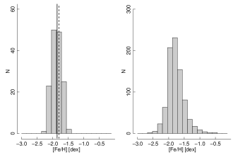
Figure 6: Distribution of the metallicities for stars (combined MSSGB and RGB sample) in M 55 (left panel) and $\omega$ Cen (right panel) as determined by our method. The dashed line is centred at $-$1.80 dex (the literature value of [Fe/H] for M 55) while the solid line denotes the mean of the distribution. There is only a small offset of 0.06 dex. The overall error for the determined metallicities in M 55 as defined in Eq. 3 is 0.15 dex.

6.1.3 Metallicity results for M 55

The metallicity values determined from the neural networks for the combined MSSGB and RGB sample are shown in the left panel in Fig. 6. These results were obtained from network model1, i.e. networks trained on all stellar parameters but with a higher weight on metallicity, see Sect. 5.1. The overall parametrization performance is good. The mean value of the metallicity distribution is $-$1.86 dex compared with a literature value of $-$1.80 dex. The overall error as defined in Eq. 3 is 0.15 dex.

Figure 7: As in Fig. 5 but for the ‘standard’ stars showing the network outputs compared to the averaged literature values for each of the parameters [Fe/H], log $g$ and $T_{\rm eff}$ (from top to bottom). The errors for the literature values are found from the scatter about the unweighted mean value for the different stated values (see Tab. 2), while the computed errors are found from 30 bootstrap networks. Note that the metallicity range on which the networks were trained was limited to values larger than $-$2.5 dex, so we cannot expect good parametrization performances for metallicities below this value. Excluding the single point with the literature value [Fe/H] = $-$2.95 dex, we find an overall average error in [Fe/H] as defined in Eq. 3 of 0.15 dex, while that for log $g$ and $T_{\rm eff}$ are 0.42 dex and 145 K respectively.

6.2 Model validation for standard stars

We compared the parameter determinations of the neural networks on standard stars with those found from other methods and listed in the catalogue of Cayrel de Strobel et al. (2001). In cases of multiple observations (from different authors) in this catalogue, we calculated the (unweighted) mean and the corresponding standard error for those values which were determined from high resolution spectroscopy. A summary of the values is given in Table 2. The network models were then validated on the spectra of these stars (see Sect. 2). We only used the networks trained for the MSSGB sample for this test (see Sect. 3). The results for log $g$ and $T_{\rm eff}$ were obtained from network model2 with a higher weight (during minimization) on surface gravity and temperature, while the results for [Fe/H] are from network model1 with a higher weight on metallicity, see Sect. 5.1. The parametrization results are summarized in Fig. 7.

From the plots we see that the metallicity results are quite good, with an overall error of less than 0.15 dex. Interestingly, the overall parametrization performance for log $g$ is not as good as for the stars in M 55, despite the fact that the S/N of the standard stars is much higher (but there are only 11 stars so the statistics is rather poor). Given that the stellar parameters of the standard stars are similar to those of the main-sequence stars in M 55, and from the fact that the input spectral ranges to the networks are identical for both types of stars, we conclude that these larger deviations are, paradoxically, related to the larger S/N. As outlined above, the S/N of the template spectra with which the networks were trained influences the degree of regularization, thus effecting the extent of systematic offsets (see Sect. 5). Indeed, the S/N of the template spectra was in the range from 10 to 100, i.e. lower than that of the standard stars. To investigate this further, we performed limited tests with networks trained on spectra with S/N values in the range from 100 to 150 while keeping the weight decay parameter fixed. We found that the systematic offset in log $g$ for the standard stars could indeed be decreased in this way (albeit not completely removed), while the variance remained almost the same. While these results support the idea of insufficient regularization, such a strong sensitivity of the network training to the S/N of the template spectra is surprising and needs to be investigated in more detail in future studies. An explanation of why there are no systematic trends for [Fe/H] is possibly given by the fact that the networks for this parameter were highly tuned, in order to eliminate inaccuracies.

Taking the stellar parameters predicted by the network for a given observed spectrum, we can generate the corresponding synthetic spectrum. Fig. 9 shows a comparison between two (observed) standard star spectra and the appropriate synthetic spectrum produced by interpolating the training sample using the stellar parameters as predicted by the neural networks. It can be seen that the model spectra represent the observed spectra rather well, especially in the case that the network’s predictions of the stellar parameters are close to the literature values.

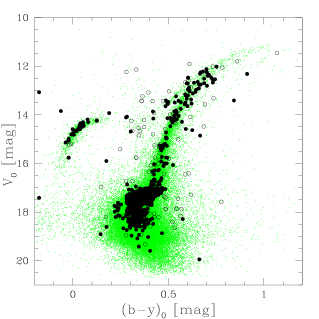
Figure 8: The spectroscopically observed stars in $\omega$ Cen are marked as heavy dots in the Strömgren colour magnitude diagram from Hilker & Richtler (2000). Based on the radial velocities, filled circles were identified as members, while open circles denote non-members.

6.3 Discussion of the parametrization results

The overall parametrization performance can be compared with that of Snider et al. (2001). They trained networks on real spectral data with similar resolutions and for stars with similar parameter ranges as in this project. They reported precisions of the parameter determinations for log $g$ of 0.25 to 0.30 dex and 135–150 K for $T_{\rm eff}$ while that for [Fe/H] was 0.15 to 0.20 dex. Our results are in absolute agreement with these values, even though our networks were trained on synthetic data.

6.4 Metallicity results for $\omega$ Cen

We applied the neural networks to the MSSGB and RGB samples of $\omega$ Cen to determine metallicities for these stars. We stress, however, that the metallicities found are somewhat preliminary and we do not attempt to give a more detailed analysis. The complex formation and evolution history of $\omega$ Cen will ultimately require a much more sophisticated approach in which synthetic spectra with different helium and/or $\alpha$ element abundances are taken into account. The results were obtained from network model1 which was tuned to improve metallicity performance. A plot of all stars observed is shown in Fig. 8. Note that we only considered the stars up to the top of the giant branch in this study (see Sect. 3), i.e. there are no HB or AGB stars. These will be examined in a future study.

The overall distribution of the metallicities found by our neural network analysis for $\omega$ Cen is shown in the right panel of Fig. 6. When compared to the distribution of metallicities found for M 55, we note a significantly larger spread. From the bootstrap errors for the metallicity values plus the smaller overall metallicity spread found for the stars in M 55 (Fig. 6), we must conclude that this large spread does not indicate an erroneous parametrization but rather a real effect of the multiple stellar populations in $\omega$ Cen.

Figure 9: A comparison of two observed standard star spectra (solid lines) with the corresponding synthetic spectra (dotted lines) as predicted by the neural network. The network predicts only the stellar parameters, but from these the synthetic spectra were generated through interpolation of the training template grid of synthetic spectra. The upper plot is for a star with stellar parameter residuals of $\Delta$([Fe/H])= $-$0.04 dex, $\Delta$(log $g$)= 0.12 dex and $\Delta$($T_{\rm eff}$)= $-$89 K, where $\Delta$ is the difference (network output $-$ literature value). The corresponding network outputs are [Fe/H] = $-$1.06 dex, log $g$= 4.16 dex and $T_{\rm eff}$= 5811 K. The lower plot shows an example were the difference between the log $g$ prediction of the network and the literature value is rather large. For this star, we find $\Delta$([Fe/H])= $-$0.01 dex, $\Delta$(log $g$)=1.11 dex and $\Delta$($T_{\rm eff}$)= 109 K and networks outputs of [Fe/H] = $-$2.15 dex, log $g$= 4.03 dex and $T_{\rm eff}$= 4984 K. The S/N of the synthetic spectra was decreased to 150, i.e. similar to that of the observed spectra.

7 Concluding Remarks

We have shown that the metallicity information in medium resolution spectra can be readily assessed by neural networks trained on synthetic spectra and without additional photometric information. The neural network approach works in an objective way and is, ultimately, time efficient, relevant when large sets of spectra of stars in different objects (clusters) are to be analysed. In order to obtain some measure of uncertainty on the stellar parameters determined, we applied the bootstrap method to neural networks for the first time for this kind of parametrization problem.

The estimated metallicity accuracies are of the order of $\sim$ 0.2 dex which is close to what one can expect from such data with any method. We additionally performed limited tests on the retrieval of log $g$ and $T_{\rm eff}$ and found that the overall accuracies for these parameters are $\sim$ 0.3 to 0.4 dex and $\sim$ 150 to 190 K. These results could probably be further improved once a suitable grid of synthetic spectra with a range of different microturbulent velocities is available. In addition, the effects of $\alpha$ abundances should be taken into account to test how well this additional parameter can be determined and whether neural networks are able to discriminate between the effects of [Fe/H] and [$\alpha$/Fe] from normalized spectra alone. Moreover, and especially with regard to $\omega$ Cen, the recent suggestions of enhanced helium abundances for the intermediate metallicity population (Norris 2004) should be taken into account in future simulations of the synthetic templates. As mentioned above, an increased helium abundance results in an overall increased molecular weight which affects the absorption lines in similar ways to log $g$.

Future tests could also include photometric data (e.g. from the pre-imaging observations). Since temperature strongly affects the continuum of a stellar energy distribution, any colour information should improve the performance for this parameter. Once a larger set of observed spectra for stars in normal globular clusters (i.e. with a well defined metallicity) is available, we will train networks on these data. Although synthetic spectra can reproduce observed stellar energy distributions rather well, we believe that a network trained on real data with similar noise and detector characteristics will result in better metallicity estimates for previously unseen data.