Quasi-Periodic Oscillations in Relativistic Tori

Abstract

Motivated by recent interesting work on p-mode oscillations in axisymmetric hydrodynamic black-hole tori by Rezzolla, Zanotti, and collaborators, I explore the robustness of these oscillations by means of two and three-dimensional relativistic hydrodynamic and MHD simulations. The primary purpose of this investigation is to determine how the amplitudes of these oscillations are affected by the presence of known instabilities of black-hole tori, including the Papaloizou-Pringle instability (PPI) and the magneto-rotational instability (MRI). Both instabilities drive accretion at rates above those considered in Rezzolla’s work. The increased accretion can allow wave energy to leak out of the torus into the hole. Furthermore, with the MRI, the presence of turbulence, which is absent in the hydrodynamic simulations, can lead to turbulent damping (or excitation) of modes. The current numerical results are preliminary, but suggest that the PPI and MRI both significantly damp acoustic oscillations in tori.

I Introduction

“Diskoseismology” (Nowak and Wagoner, 1991) is a relatively new subfield of accretion disk physics. Often diskoseismic oscillations have been overlooked as uninteresting because, to be observable from the outside, they must be trapped in a particular region of the disk or have a global pattern. For a Keplerian disk in a Newtonian potential, there are no global modes and relatively few trapped modes. Relativistic gravity helps the situation somewhat by providing a richer set of trapped modes. Nevertheless, even in general relativity, Keplerian thin disks have only a few trapped modes, which mostly occur in very restricted regions of the disk.

Non-Keplerian disks, on the other hand, have a much richer set of diskoseismic modes available for two fundamental reasons. First, in contrast to Keplerian disks, which in principle extend to infinity, non-Keplerian disks can be constructed to have a finite size and can thus act as a single resonant cavity. Second, unlike Keplerian disks, non-Keplerian disks necessarily have radial pressure gradients that can provide an additional restoring force (along with the centrifugal force and gravity) in support of oscillations.

In this work I focus on inertial-acoustic (p-mode) oscillations in finite tori. Two interesting consequences of such oscillations have previously been identified. First, they can cause periodic changes in the mass quadrupole moment of the disks. For massive tori of nearly nuclear densities, this may produce gravitational radiation detectable by LIGO, especially for sources located within our galaxy (Zanotti et al., 2003). Such massive tori could form from the gravitational collapse of a massive rotating star or as an intermediate state in a binary neutron star merger. These oscillations may also be important in explaining quasi-periodic oscillations (QPOs), particularly the harmonically related high-frequency QPOs (HFQPOs) seen in some black-hole candidate low-mass X-ray binaries (LMXBs) (Rezzolla et al., 2003).

My goal here is to extend previous numerical simulations of oscillating tori (Zanotti et al., 2003, 2005) to include magnetic fields and nonaxisymmetric perturbations. I proceed in §II by reviewing the equations of general relativistic magnetohydrodynamics as solved in the numerical code used in this work. The code itself is briefly described in §III. In §IV I present the results of this study. I conclude with some final thoughts in §V.

II General Relativistic MHD Equations

This work uses a form of the general relativistic MHD equations similar to De Villiers and Hawley (2003a). Nevertheless, it is worth explicitly writing these equations out for clarity. In flux-conserving form, the conservation equations for mass, internal energy, and momentum and the induction equation for magnetic fields are:

$$\frac{\partial D}{\partial t}+\frac{\partial(DV^{i})}{\partial x^{i}} = 0,$$ (1)

$$\frac{\partial E}{\partial t}+\frac{\partial(EV^{i})}{\partial x^{i}} = -P\frac{\partial W}{\partial t}-P\frac{\partial(WV^{i})}{\partial x^{i}},$$ (2)

$$\frac{\partial S_{j}}{\partial t}+\frac{\partial(S_{j}V^{i})}{\partial x^{i}} = \frac{\partial(\sqrt{-g}B_{j}B^{0}/{4\pi})}{\partial t}$$

$${}+\frac{\partial(\sqrt{-g}B_{j}B^{i}/{4\pi})}{\partial x^{i}}$$

$${}+\frac{1}{2}\left(\frac{S^{\mu}S^{\nu}}{S^{0}}-\frac{\sqrt{-g}}{4\pi}B^{\mu}B^{\nu}\right)\frac{\partial g_{\mu\nu}}{\partial x^{j}}$$

$${}-\sqrt{-g}\frac{\partial(P+||B||^{2}/{8\pi})}{\partial x^{j}},$$

$$\frac{\partial\mathcal{B}^{i}}{\partial t}+\frac{\partial(\mathcal{B}^{i}V^{j})}{\partial x^{j}} = \mathcal{B}^{j}\frac{\partial V^{i}}{\partial x^{j}},$$ (4)

where $g$ is the determinant of the 4-metric, $W=\sqrt{-g}u^{t}$ is the relativistic boost factor, $D=W\rho$ is the generalized fluid density, $P=(\Gamma-1)E/W$ is the fluid pressure, $V^{i}=u^{i}/u^{t}$ is the transport velocity, $S_{i}=W\rho hu_{i}$ is the covariant momentum density, and $E=We=W\rho\epsilon$ is the generalized internal energy density. There are two representations of the magnetic field in these equations: $B^{\mu}$ is the magnetic field 4-vector ($||B||^{2}=g_{\mu\nu}B^{\mu}B^{\nu}$) and

$$\mathcal{B}^{\mu}=W(B^{\mu}-B^{0}V^{\mu})$$ (5)

is the divergence-free ($\partial\mathcal{B}^{i}/\partial x^{i}=0$), spatial ($\mathcal{B}^{0}=0$) representation of the field. The time component of the magnetic field $B^{0}$ is recovered from the orthogonality condition $B^{\mu}u_{\mu}=0$.

These equations are evolved in a Kerr-Schild polar coordinate system $({t},{r},{\theta},{\phi})$, although all of the simulations in this work assume a non-rotating ($a=0$) Schwarzschild black hole. The computational advantages of the “horizon-adapted” Kerr-Schild form of the Kerr metric are described in Papadopoulos and Font (1998) and Font et al. (1998). The primary advantage is that, unlike Boyer-Lindquist coordinates, there are no singularities in the metric terms at the event horizon. This is particularly important for numerical calculations as it allows one to place the grid boundaries inside the horizon, thus ensuring that they are causally disconnected from the rest of the flow.

III Numerical Method

These simulations are carried out using the numerical code Cosmos++, a massively parallel, multidimensional (one, two, or three dimensions), adaptive-mesh, magnetohydrodynamic code for evolving both Newtonian and relativistic flows. Cosmos++ employs a time-explicit, operator-split, finite volume discretization method with second-order spatial accuracy. A detailed description of Cosmos++, including test results, will be presented in an upcoming paper.

The simulations are initialized with the analytic solution for an axisymmetric torus with constant specific angular momentum $l$. For the initialization, we assume an isentropic equation of state $P=\kappa\rho^{\Gamma}$, although during the evolution, the adiabatic form $P=(\Gamma-1)E/W$ is used to recover the pressure when solving equations (2) and (II). We set $\Gamma=4/3$ and $\kappa=0.0229$ (in $G=c=1$ units).

This work presents both two-dimensional (axisymmetric) and three-dimensional simulations. The two-dimensional simulations are carried out on a grid extending from $0.98r_{BH}\leq r\leq r_{max}$ and $0\leq\theta\leq\pi$, where $r_{BH}=2GM/c^{2}$ is the radius of the black-hole horizon. The three-dimensional simulations include the full azimuthal range $0\leq\phi<2\pi$. We choose $r_{max}$ to be about twice the initial outer radius $r_{out}$ of the torus. In order to increase the resolution inside the torus, we replace the radial coordinate ${r}$ with a logarithmic coordinate $x_{1}=1+\ln(r/r_{BH})$ and the angular coordinate $\theta$ with a coordinate $x_{2}$ satisfying $\theta=x_{2}+\frac{1}{4}\sin(2x_{2})$. The grid is resolved with $128\times 128$ zones in 2D, giving a radial spacing of $0.04r_{G}$ near the horizon and $0.6r_{G}$ near the outer boundary. In the present work, the 3D simulations are limited to $64^{3}$ zones.

In the “background” regions not determined by the initial torus solution, we initialize the gas following the spherical Bondi accretion solution (Michel, 1972). We fix the parameters of this solution such that the rest mass present in the background is negligible compared to the mass in the torus. The outer radial boundary is held fixed with the analytic Bondi solution for all evolved fields. The inner radial boundary uses outflow ($V^{r}<0$) boundary conditions. Data are shared appropriately across angular boundaries.

IV Results

Results are presented in geometrized units ($G=c=1$) with units of length parameterized in terms of the gravitational radius of the black hole, $r_{G}=GM/c^{2}$.

IV.1 2D Axisymmetric Hydro

It is instructive to begin this work by reproducing the results of a previously published axisymmetric hydrodynamic simulation of an oscillating torus. This will be useful for illustrating how p-mode oscillations are generally manifested in axisymmetric hydrodynamic tori and facilitate easier comparison with the subsequent MHD and non-axisymmetric results. This is also important as a validation of the new code used here. I choose Model (a) from Zanotti et al. (2003) for this purpose. In this model, the specific angular momentum, which is constant throughout the torus, is $l/M=3.8$. The torus just fills the largest closed equipotential surface so that the inner torus boundary corresponds with the location of the cusp $r_{in}=r_{cusp}=4.576$. The outer radius for such a torus is $r_{out}=15.889$. The density center of this torus is located at $r_{center}=8.352$; the orbital period at this radius is $t_{orb}=151.7$. This will serve as a reference dynamical timescale for all these simulations. To excite the resonant acoustic mode I use an initial radial velocity kick. For convenience this velocity is set at a small fraction ($\eta=0.12$) of the background Bondi inflow velocity.

I use the $L_{2}$ norm of the rest mass density, defined as $||\rho||^{2}=\sum_{i=1}^{N_{r}}\sum_{j=1}^{N_{\theta}}\rho_{ij}^{2}$, to characterized the global oscillatory behavior of the torus. The time history and Fourier power spectrum of this quantity are shown in Figures 1 and 2, respectively. The power spectrum, in particular, reveals the rich harmonic structure characteristic of diskoseismic modes (Kato, 2001). Rezzolla et al. (2003) also showed that this structure is consistent with predictions of linear perturbation analysis of vertically integrated relativistic tori.

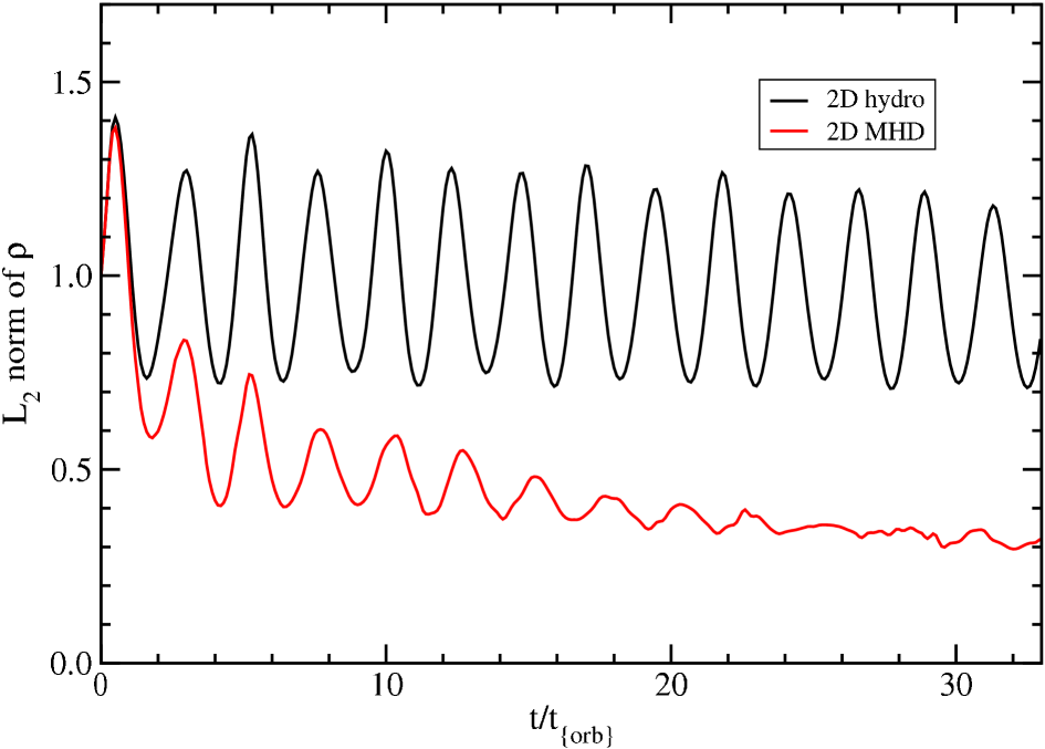
Figure 1: Time history of the $L_{2}$ norm of the rest-mass density. The vertical scale has been adjusted to the initial value of $||\rho||^{2}$.

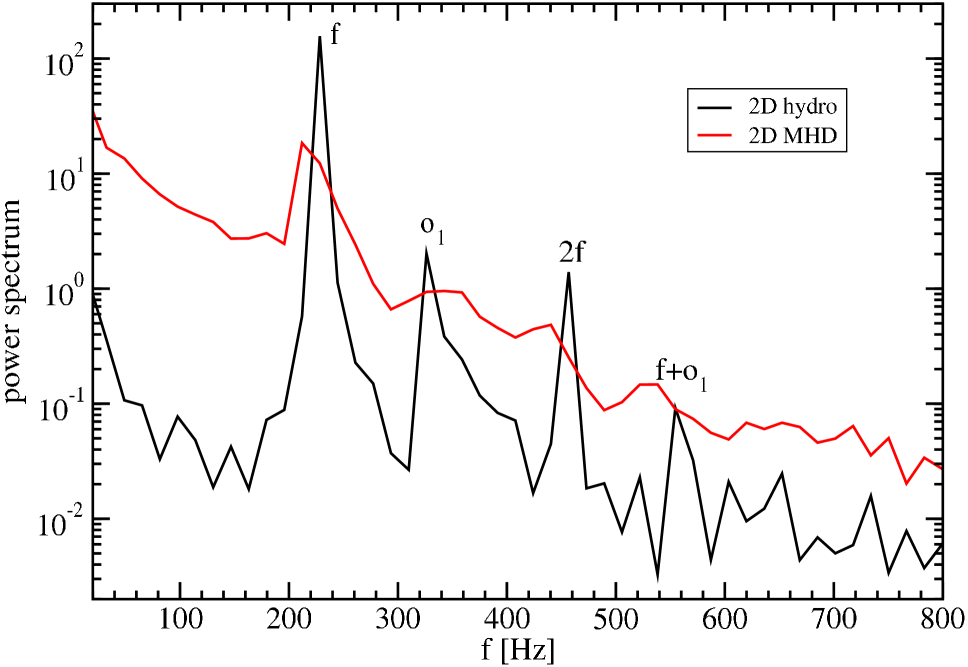
Figure 2: Power spectra of the $L_{2}$ norm of the rest-mass density. The spectra have been arbitrarily normalized such that the strongest frequency bin has a value of 100. The frequency is set assuming a black hole mass $M_{BH}=2.5M_{\odot}$.

Although the p-mode of interest in this work is an acoustic wave within the disk, the torus parameters for this model are such that this wave periodically pushes material over the cusp and out of the torus. This material is accreted into the black hole on a dynamical timescale. Therefore, one manifestation of the p-mode in (marginally stable) tori is a periodic fluctuation in the black-hole mass accretion rate as shown in Figure 3. The Fourier power spectrum of the accretion history (Figure 4) reveals the same fundamental frequency and first overtone as Figure 2, confirming the connection.

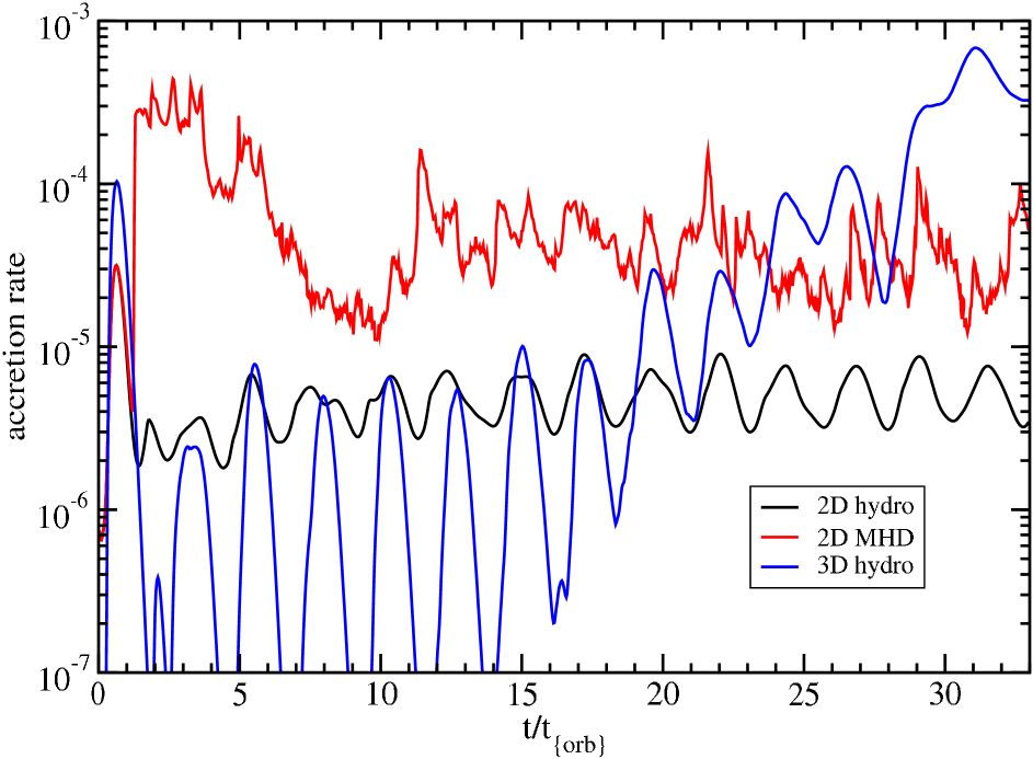
Figure 3: Rest mass accretion rate normalized by the initial mass of the torus.

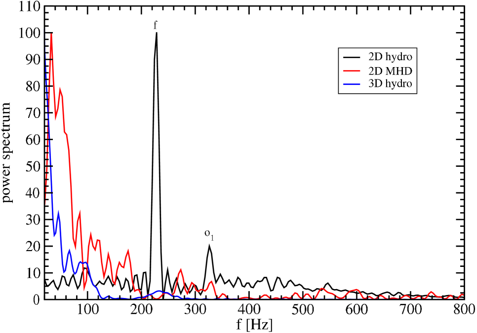
Figure 4: Power spectra of the mass accretion rate. The spectra have been arbitrarily normalized such that the strongest frequency bin has a value of 100. The frequency is set assuming a black hole mass $M_{BH}=2.5M_{\odot}$.

IV.2 3D Hydro

I now drop the restriction of axisymmetry and consider a three-dimensional hydrodynamic torus. The concern here is that such a structure is known to be unstable to low-order non-axisymmetric modes (the Papaloizou-Pringle instability or PPI). Note that this simulation uses a slightly different initial setup than the previous one. First, the velocity perturbation is slightly smaller in this case ($\eta=0.06$ instead of 0.12). In my testing I have found that the amplitude of this perturbation has little effect on the results, so this difference shouldn’t be important. This simulation also uses a different set of parameters for the background Bondi solution. These differences account for the much larger amplitude of oscillations in the accretion rate for the three-dimensional model (Figure 3). Nevertheless, the frequency of the oscillations in both cases is the same, indicating that the different background treatments do not effect the behavior of the p-mode oscillations.

It is useful for this simulation to add a diagnostic to track the growth of the main PPI modes. We extract the $m=1$ and 2 modes by computing azimuthal density averages as (De Villiers and Hawley, 2002)

$$\mathrm{Re}[k_{m}(r)]=\int_{0}^{2\pi}\rho(r,\pi/2,\phi)\cos(m\phi)d\phi~{},$$ (6)

$$\mathrm{Im}[k_{m}(r)]=\int_{0}^{2\pi}\rho(r,\pi/2,\phi)\sin(m\phi)d\phi~{}.$$ (7)

The power in mode $m$ is then

$$f_{m} = \frac{1}{r_{max}-r_{min}}\int_{r_{min}}^{r_{max}}\ln\left[\left(\left\{\mathrm{Re}[k_{m}(r)]\right\}^{2}\right.\right.$$

$${}+\left.\left.\left\{\mathrm{Im}[k_{m}(r)]\right\}^{2}\right)\right]dr~{},$$

where $r_{min}$ and $r_{max}$ are the approximate inner and outer edges of the disk. In Figure 5 we show the growth of these two modes as a function of time. As expected, there is significant mode growth for this slender torus. Furthermore, this mode growth does not appear to saturate before the end of the simulation. Figure 6 shows the midplane density of this model at $t/t_{orb}=33$. An $m=1$ “planet” and inflowing spiral wave are both apparent.

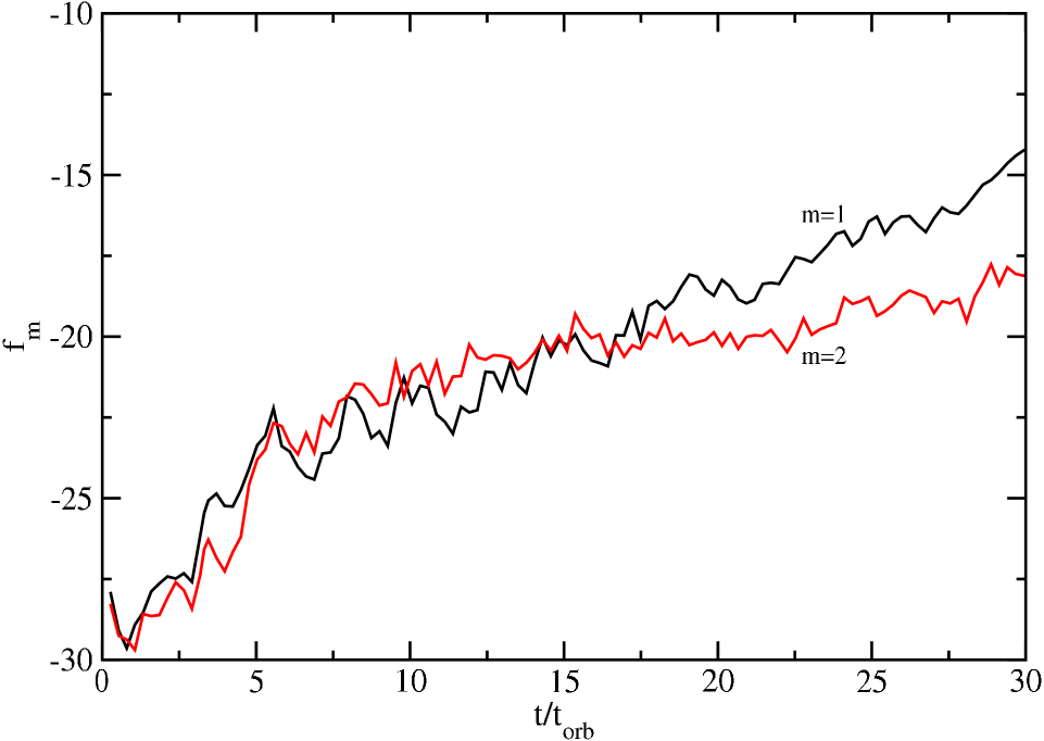
Figure 5: PPI mode growth.

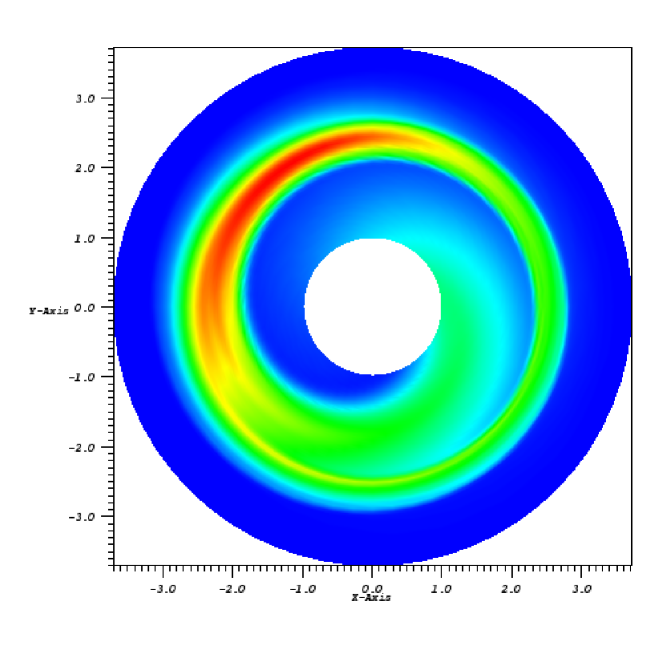
Figure 6: Density in the midplane of the torus. This plot is shown using the logarithmic radial coordinate.

The question of interest now is what effect this PPI growth has on the p-mode oscillations. From Figure 3 it is clear that the PPI growth coincides with a significant increase in the mass accretion rate, due to the angular momentum transport of the spiral waves generated in the torus. Despite the very significant changes to the structure of the torus, the fundamental p-mode is able to survive at least to the end of this simulation, as is apparent in Figure 3. However, the power in this mode is significantly reduced and it is smeared out in frequency space as shown in Figure 4. The frequency broadening is probably due to changes in the internal structure of the torus. The damping is probably a result of leaking wave energy into the black hole along the accretion stream.

IV.3 2D Axisymmetric MHD

I now explore the effect of adding initially weak poloidal magnetic field loops to the axisymmetric torus investigated in §IV.1. The presence of the poloidal field triggers the violent growth of the magneto-rotational instability (MRI Balbus and Hawley, 1991; Hawley, 1991). The MRI facilitates angular momentum transport through magnetohydrodynamic turbulence. Similar to §IV.2, the focus here is to determine whether the p-mode oscillations seen in the 2D hydrodynamic simulation can survive in the presence of a known instability, in this case the MRI.

The initial magnetic field vector potential is (De Villiers and Hawley, 2003a)

$$A_{\phi}=\left\{\begin{array}[]{ccc}k(\rho-\rho_{min})&\mathrm{for}&\rho\geq\rho_{min}~{},\\ 0&\mathrm{for}&\rho<\rho_{min}~{}.\end{array}\right.$$ (9)

The non-zero spatial magnetic field components are then $\mathcal{B}^{r}=-\partial_{\theta}A_{\phi}$ and $\mathcal{B}^{\theta}=\partial_{r}A_{\phi}$. These poloidal field loops coincide with the isodensity contours of the torus. The constant $k$ is normalized such that initially $\beta=P/(||B||^{2}/8\pi)\geq 100$ throughout the torus. The parameter $\rho_{min}=0.5*\rho_{center}$ is used to keep the field a suitable distance inside the surface of the torus.

The presence of MRI turbulence dramatically increases the mass accretion rate compared to the hydrodynamic torus (see Figure 3) and also redistributes the disk material into a broader, more radially extended structure as shown in Figure 7. It is important to note that axisymmetric MRI simulations are susceptible to a particularly violent form of the poloidal MRI, called the channel solution (Hawley and Balbus, 1992), which can itself lead to highly episodic mass accretion (cf. De Villiers and Hawley, 2003b), apparent in Figure 3.

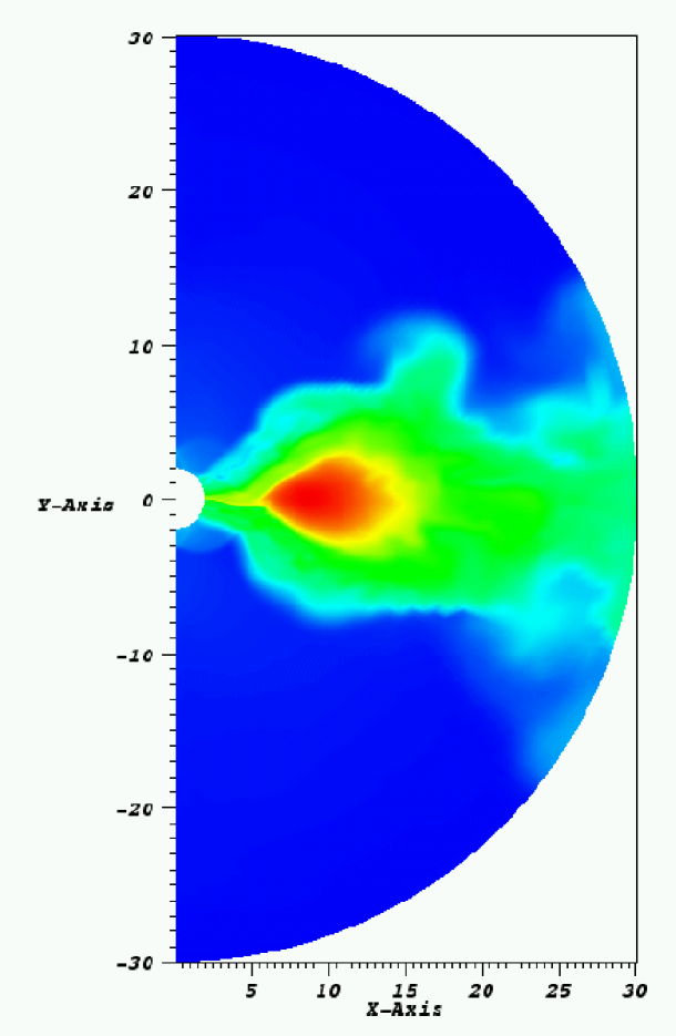
Figure 7: Logarithm of density for the initial and final torus states for the 2D MHD simulation.

Comparisons of the power spectra of the $L_{2}$ density norms (Figure 2) and mass accretion rates (Figure 4) suggest that the violent nature of the channel solution strongly damps the p-mode oscillations. The accretion spectrum of this simulation shows no power in the fundamental mode or its overtones. The $L_{2}$ density norm spectrum shows some power in the fundamental mode, although the amplitude of the oscillation decays with time, as apparent in Figure 1. It remains to be seen if this strong damping is restricted to the onset of the MRI or is a more general feature of these turbulent tori.

V Summary

An obvious extension of this work will be to perform 3D MHD simulations. There are two potentially important differences between magnetized axisymmetric (2D) and nonaxisymmetric (3D) tori. One is the fact that the very violent channel solution of MRI (seen in Figure 7) is itself susceptible to a nonaxisymmetric instability that destroys its coherence (Goodman and Xu, 1994). As a consequence, accretion from a nonaxisymmetric torus is much less episodic than the equivalent 2D torus (De Villiers and Hawley, 2003b). The second is that the MRI is unable to sustain itself through dynamo action in axisymmetry. The sustained activity of the MRI in three-dimensions will be important in assessing the importance of p-mode oscillations in magnetized relativistic tori.

If acoustic modes are indeed strongly damped in turbulent MRI disks, then the puzzle of QPOs in black-hole X-ray binaries becomes more problematic. The MRI only requires that a disk be differentially rotating at a rate that decreases with radial distance and that it have a weak magnetic field. Both of these conditions are thought to be generally met in astrophysical accretion disks. In light of this and the results presented here, it appears that p-mode oscillations may not be a viable mechanism for generating observable QPOs in realistic accretion disks, but 3D MHD simulations will be necessary to confirm this.

Animated movies of these results are available at
http://www.physics.ucsb.edu/$\sim$fragile/research.html.