Gravitational Radiation from an Accreting Millisecond Pulsar with a Magnetically Confined Mountain

Abstract

The amplitude of the gravitational radiation from an accreting neutron star undergoing polar magnetic burial is calculated. During accretion, the magnetic field of a neutron star is compressed into a narrow belt at the magnetic equator by material spreading equatorward from the polar cap. In turn, the compressed field confines the accreted material in a polar mountain which is misaligned with the rotation axis in general, producing gravitational waves. The equilibrium hydromagnetic structure of the polar mountain, and its associated mass quadrupole moment, are computed as functions of the accreted mass, $M_{\rm a}$, by solving a Grad-Shafranov boundary value problem. The orientation- and polarization-averaged gravitational wave strain at Earth is found to be $h_{\rm c}=6\times 10^{-24}(M_{\rm a}/M_{\rm c})(1+M_{\rm a}b^{2}/8M_{\rm c})^{-1}(f/0.6\,{\rm kHz})^{2}(d/1\,{\rm kpc})^{-1}$, where $f$ is the wave frequency, $d$ is the distance to the source, $b$ is the ratio of the hemispheric to polar magnetic flux, and the cut-off mass $M_{\rm c}\sim 10^{-5}M_{\sun}$ is a function of the natal magnetic field, temperature, and electrical conductivity of the crust. This value of $h_{\rm c}$ exceeds previous estimates that failed to treat equatorward spreading and flux freezing self-consistently. It is concluded that an accreting millisecond pulsar emits a persistent, sinusoidal gravitational wave signal at levels detectable, in principle, by long baseline interferometers after phase-coherent integration, provided that the polar mountain is hydromagnetically stable. Magnetic burial also reduces the magnetic dipole moment $\mu$ monotonically as $\mu\propto(1+3M_{\rm a}/4M_{\rm c})^{-1}$, implying a novel, observationally testable scaling $h_{\rm c}(\mu)$. The implications for the rotational evolution of (accreting) X-ray and (isolated) radio millisecond pulsars are explored.

1 Introduction

The current generations of resonant bar antennas and long baseline interferometers are capable of detecting gravitational wave signals from incoherent sources with strain amplitudes $h$ exceeding $\sim 10^{-20}$ and $\sim 10^{-21}$ respectively at frequencies near $f\approx 0.6\,{\rm kHz}$ (Schutz, 1999). The sensitivity can be improved by a factor $(f\tau)^{1/2}$ for periodic sources of known $f$ by integrating coherently for a total observing time $\tau$, as in heirarchical Fourier searches (Dhurandhar et al., 1996; Brady et al., 1998; Brady & Creighton, 2000). Several classes of sources with promising event rates have been identified in the kilohertz regime: coalescing neutron-star binaries (Phinney, 1991), r-modes in young, hot neutron stars (Andersson, 1998; Lindblom et al., 1998), and neutron stars in low-mass X-ray binaries whose crusts are deformed by temperature gradients (Bildsten, 1998; Ushomirsky et al., 2000). More generally, every isolated and accreting millisecond pulsar is potentially a kilohertz source, because the stellar magnetic field, which is usually not symmetric about the rotation axis, deforms the crust and interior hydromagnetically. It is presently believed that hydromagnetic deformations are too small to produce gravitational waves detectable by the current generation of interferometers, with $h\sim 10^{-31}(B/10^{12}\,{\rm G})^{2}(f/0.6\,{\rm kHz})^{2}(d/1\,{\rm kpc})^{-1}$ for an object with surface magnetic field $B$, situated at a distance $d$ from Earth (Katz, 1989; Bonazzola & Gourgoulhon, 1996). Magnetars, with $B\gtrsim 10^{15}\,{\rm G}$, are invoked as a possible exception (Konno et al., 2000; Ioka, 2001; Palomba, 2001), as are objects whose internal toroidal fields are many times greater than $B$ (Cutler, 2002), or whose macroscopically averaged Maxwell stress tensor is enhanced relative to uniform magnetization because the internal field is concentrated in flux tubes, e.g. in a type II superconductor (Jones, 1975; Bonazzola & Gourgoulhon, 1996).

In this paper, we show that previous calculations materially underestimate the hydromagnetic deformation of recycled pulsars, e.g. accreting millisecond pulsars such as SAX J1808.4$-$3658 (Wijnands & van der Klis, 1998; Chakrabarty & Morgan, 1998; Galloway et al., 2002; Markwardt et al., 2002). During accretion, in a process termed magnetic burial, material spreads equatorward from the polar cap, compressing the magnetic field into a narrow belt at the magnetic equator and increasing the field strength locally while reducing the global dipole moment $\mu$ (Melatos & Phinney, 2000, 2001; Payne & Melatos, 2004), in accord with observations of low- and high-mass X-ray binaries and binary radio pulsars (Taam & van de Heuvel, 1986; van den Heuvel & Bitzaraki, 1995). In turn, the compressed equatorial magnetic field reacts back on the accreted material, confining it in a polar mountain which is misaligned with the rotation axis in general (Melatos & Phinney, 2000, 2001). The gravitational ellipticity $\epsilon$ (Brady et al., 1998) of the mountain, calculated here self-consistently, can approach $\epsilon\sim 10^{-7}$, materially greater than for an undistorted dipole [$\epsilon\approx 6\times 10^{-13}(B/10^{12}\,{\rm G})^{2}$, e.g. Katz (1989)] due to the enhanced stress from the compressed field. A mountain of this size generates gravitational waves at levels detectable by the current generation of interferometers and can explain the observed clustering of the spin periods of accreting millisecond pulsars through the stalling effect discovered by Bildsten (1998).

In §2, we review the physics of magnetic burial and calculate the hydromagnetic structure of the polar mountain as a function of accreted mass $M_{\rm a}$ by solving an appropriate Grad-Shafranov boundary value problem, connecting the initial and final states self-consistently, and treating Ohmic diffusion semiquantitatively (Melatos & Phinney, 2001; Payne & Melatos, 2004). In §3, we predict the orientation- and polarization-averaged gravitational wave strain $h_{\rm c}(M_{\rm a})$ and compare it against the sensitivity of the Laser Interferometer Gravitational-Wave Observatory (LIGO). We also combine $h_{\rm c}(M_{\rm a})$ with $\mu(M_{\rm a})$ from previous work (Payne & Melatos, 2004) to deduce a novel, observationally testable scaling $h_{\rm c}(\mu)$ for accreting millisecond pulsars (Melatos & Phinney, 2000). In §4, we discuss the implications of magnetic burial for the sign of the net torque acting on an X-ray millisecond pulsar and the evolution of $h_{\rm c}$ and $\mu$ after accretion ends (e.g. in radio millisecond pulsars). Our conclusions rely on the assumption that the polar mountain is not disrupted by hydromagnetic (e.g. Parker) instabilities; the justification of this assumption is postponed to future work. Deformation by magnetic burial also occurs in white dwarfs (Katz, 1989; Heyl, 2000; Cumming, 2002).

2 Polar magnetic burial

2.1 Equilibrium hydromagnetic structure of the polar mountain

The equilibrium mass density $\rho({\bf x})$ and magnetic field intensity ${\bf B}({\bf x})$ in the polar mountain are determined by the equation of hydromagnetic force balance,

$$\nabla p+\rho\nabla\phi-(4\pi)^{-1}(\nabla\times{\bf B})\times{\bf B}=0~{},$$ (1)

supplemented by (i) the condition $\nabla\cdot{\bf B}=0$, (ii) the gravitational potential $\phi$ (with $|\nabla\phi|\approx GM_{\ast}/R_{\ast}^{2}$, where $M_{\ast}$ and $R_{\ast}$ are the stellar mass and radius, because the mountain is much shorter than $R_{\ast}$), and (iii) an equation of state for the pressure $p$ (isothermal for simplicity, i.e. $p=c_{\rm s}^{2}\rho$, where $c_{\rm s}$ is the sound speed). We define spherical polar coordinates $(r,\theta,\phi)$, such that $\theta=0$ coincides with the magnetic axis before accretion, and we seek solutions to (1) that are symmetric about this axis, such that ${\bf B}$ can be constructed from a scalar flux function $\psi(r,\theta)$ according to ${\bf B}=(r\sin\theta)^{-1}\nabla\psi\times{\bf\hat{e}}_{\phi}$. Upon resolving (1) into components parallel and perpendicular to ${\bf B}$, we arrive respectively at the barometric formula $\rho=c_{\rm s}^{-2}F(\psi)\exp[-(\phi-\phi_{0})/c_{\rm s}^{2}]$, with $\phi_{0}=GM_{\ast}/R_{\ast}$, and the Grad-Shafranov equation describing cross-field force balance (Hameury et al., 1983; Brown & Bildsten, 1998; Litwin et al., 2001; Melatos & Phinney, 2001; Payne & Melatos, 2004),

$$\frac{\partial^{2}\psi}{\partial r^{2}}+\frac{\sin\theta}{r^{2}}\frac{\partial}{\partial\theta}\left(\frac{1}{\sin\theta}\frac{\partial\psi}{\partial\theta}\right)=-4\pi r^{2}\sin^{2}\theta F^{\prime}(\psi)\exp[-(\phi-\phi_{0})/c_{\rm s}^{2}]~{}.$$ (2)

It is customary to choose an arbitrary (albeit physically plausible) functional form of $F(\psi)$ in order to solve (2) (Uchida & Low, 1981; Hameury et al., 1983; Brown & Bildsten, 1998; Litwin et al., 2001). However, this approach leads to an inconsistency. In the perfectly conducting limit, material is frozen to magnetic field lines. Hence the mass $dM=2\pi d\psi\int ds\,\rho[r(s),\theta(s)]r\sin\theta|\nabla\psi|^{-1}$ enclosed between two adjacent flux surfaces $\psi$ and $\psi+d\psi$ (where the integral is along a field line) equals the mass enclosed before accretion plus any mass added during accretion, without any cross-field transport of material (Mouschovias, 1974; Melatos & Phinney, 2001; Payne & Melatos, 2004). To calculate $\psi$ correctly, one must specify $dM/d\psi$ according to the global accretion physics, with $F(\psi)$ following from

$$F(\psi)=\frac{c_{\rm s}^{2}}{2\pi}\frac{dM}{d\psi}\left\{\int ds\,r\sin\theta|\nabla\psi|^{-1}\exp[-(\phi-\phi_{0})/c_{\rm s}^{2}]\right\}^{-1};$$ (3)

otherwise, if $F(\psi)$ is specified, $dM/d\psi$ changes as a function of $M_{\rm a}$ in a manner that inconsistently leads to cross-field transport. The functional form of $F(\psi)$, determined self-consistently through (3), changes as $M_{\rm a}$ increases. This property, newly recognized in the context of magnetic burial (Melatos & Phinney, 2001; Payne & Melatos, 2004), has an important astrophysical consequence: it produces a greater hydromagnetic deformation than predicted by previous authors, because polar (accreting) and equatorial (nonaccreting) flux tubes maintain strictly separate identities through (3), without exchanging material, and hence the equatorial magnetic field is highly compressed.

We solve (2) and (3) simultaneously for $\psi(r,\theta)$ and $\rho(r,\theta)$ subject to the line-tying (Dirichlet) boundary condition $\psi(R_{\ast},\theta)=\psi_{\ast}\sin^{2}\theta$ at the stellar surface, such that the footpoints of magnetic field lines are anchored to the heavy, highly conducting crust (Melatos & Phinney, 2001; Payne & Melatos, 2004). We adopt a mass-flux distribution, $M(\psi)=\text@frac{1}{2}M_{\rm a}(1-e^{-\psi/\psi_{\rm a}})(1-e^{-\psi_{\ast}/\psi_{\rm a}})^{-1}$, that embodies the essence of disk accretion, namely that the accreted mass is distributed rather evenly within the polar flux tube $0\leq\psi\leq\psi_{\rm a}$, with minimal leakage onto equatorial flux surfaces $\psi_{\rm a}\leq\psi\leq\psi_{\ast}$, where $\psi_{\ast}=\psi(R_{\ast},\pi/2)$ denotes the hemispheric flux and $\psi_{\rm a}$ is the flux surface touching the inner edge of the accretion disk (radius $R_{\rm a}$). Payne & Melatos (2004) verified that the results do not depend sensitively on the exact form of $M(\psi)$, only on the ratio $\psi_{\rm a}/\psi_{\ast}$.

The boundary value problem (2) and (3) with surface line-tying can be solved analytically, in the small-$M_{\rm a}$ limit, by Green functions after approximating the source term on the right-hand side of (2) to sever the coupling between (2) and (3) (Payne & Melatos, 2004). It can also be solved numerically by an iterative scheme that solves the Poisson equation (2) for a trial source term by successive overrelaxation then updates $F(\psi)$ from (3) by integrating numerically along a set of contours (including closed and edge-interrupted loops) (Mouschovias, 1974; Payne & Melatos, 2004). The numerical scheme is valid for arbitrarily large $M_{\rm a}$, although convergence deteriorates as $M_{\rm a}$ increases. Typically, we use a $256\times 256$ grid and $255$ contours (linearly or logarithmically spaced) and target an accuracy of $|\Delta\psi/\psi|\leq 10^{-2}$ after $\sim 10^{3}$ iterations. We rescale the $r$ and $\theta$ coordinates logarithmically in the regions where steep gradients develop, e.g. $\theta\approx\pi/2$ (Payne & Melatos, 2004).

2.2 Ohmic diffusion

The structure of the polar mountain evolves quasistatically, over many Alfvén times, in response to (i) accretion, which builds up the mountain against the confining stress of the compressed equatorial magnetic field, and (ii) Ohmic diffusion, which enables the mountain to relax equatorward as magnetic field lines slip through the resistive fluid. The competition between accretion and Ohmic diffusion has been studied in detail in the context of neutron stars (Brown & Bildsten, 1998; Litwin et al., 2001; Cumming et al., 2001) and white dwarfs (Cumming, 2002). In these papers, steady-state, one-dimensional profiles of the magnetic field are computed as functions of depth, from the ocean down to the outer crust, and the Ohmic ($t_{\rm d}$) and accretion ($t_{\rm a}$) time-scales are compared, under the assumptions that the magnetic field is flattened parallel to the surface by polar magnetic burial, the accreted material is unmagnetized, and the accretion is spherical; ‘the complex problem of the subsequent spreading of matter’ is not tackled (Cumming, 2002). The field penetrates the accreted layer if the accretion rate satisfies $\dot{M}_{\rm a}\lesssim 0.1\dot{M}_{\rm Edd}$, where $\dot{M}_{\rm Edd}$ is the Eddington rate, but it is screened diamagnetically (i.e. buried) if $\dot{M}_{\rm a}\gtrsim 0.1\dot{M}_{\rm Edd}$, such that the surface field is reduced $\approx(\dot{M}_{\rm a}/0.002\dot{M}_{\rm Edd})$-fold relative to the base of the crust (Cumming et al., 2001).

In the regime $t_{\rm d}\lesssim t_{\rm a}$, Ohmic diffusion outpaces accretion. As material is added, it does not compress the equatorial magnetic field further; instead, it diffuses across field gradients and distributes itself uniformly over the stellar surface. Hence the polar mountain (i.e. the asymmetric component of $\rho$) ‘stagnates’ at the structure attained when $t_{\rm d}\sim t_{\rm a}$. The accretion time-scale is defined as $t_{\rm a}=M_{\rm a}/\dot{M}_{\rm a}$. The Ohmic diffusion time-scale is given by $t_{\rm d}=4\pi\sigma L^{2}/c^{2}$, where $\sigma$ denotes the electrical conductivity and $L=(|\psi|/|\nabla\psi|)_{\rm min}$ is the characteristic length-scale of the steepest field gradients; $L$ reduces to the hydrostatic scale-height in the one-dimensional geometry employed in earlier work (Brown & Bildsten, 1998; Cumming et al., 2001; Cumming, 2002) but is dominated by latitudinal gradients here. Following Cumming et al. (2001), we assume that the electrical resistivity is dominated by electron-phonon scattering in the outer crust ($M_{\rm a}\gtrsim 10^{-10}M_{\sun}$), as expected if the crustal composition is primordial, although electron-impurity scattering may dominate if the products of hydrogen/helium burning leach into the crust. In the relaxation time approximation, with all Coulomb logarithms set to unity, the electron-phonon conductivity is given by $\sigma=7.6\times 10^{26}(\rho/10^{11}\,{\rm g\,cm^{-3}})(\nu_{\rm c}/10^{16}\,{\rm s^{-1}})^{-1}(m_{\rm eff}/m_{\rm e})^{-1}(A/2)^{-1}\,{\rm s^{-1}}$, where $A$ and $Z$ denote the mean molecular weight and atomic number per electron, $m_{\rm eff}$ is the effective electron mass, $\nu_{\rm c}=1.2\times 10^{18}(T/10^{8}\,{\rm K})\,{\rm s^{-1}}$ is the electron-phonon collision frequency, $T$ is the temperature of the crust, and $\rho=6.2\times 10^{10}AZ^{-1}(M_{\rm a}/10^{-5}M_{\sun})^{3/4}\,{\rm g\,cm^{-3}}$ is the density at the base of the accreted layer (Brown & Bildsten, 1998; Cumming et al., 2001). Ohmic diffusion therefore arrests the growth of the polar mountain for

$$\frac{|\psi|}{|\nabla\psi|}\lesssim 4.2\times 10^{2}Z^{1/2}\left(\frac{M_{\rm a}}{10^{-5}M_{\sun}}\right)^{1/8}\left(\frac{T}{10^{8}\,{\rm K}}\right)^{1/2}\left(\frac{m_{\rm eff}}{m_{\rm e}}\right)^{1/2}\left(\frac{\dot{M}_{\rm a}}{\dot{M}_{\rm Edd}}\right)^{-1/2}{\rm cm}~{},$$ (4)

corresponding to the condition $t_{\rm d}\leq t_{\rm a}$. The left-hand side of (4) is computed directly from the numerical solution, by scanning over the grid, or from the approximate analytic solution in §2.3; it depends implicitly on $M_{\rm a}$. We denote by $M_{\rm d}$ the minimum accreted mass for which (4) is satisfied. Note that $t_{\rm d}/t_{\rm a}$ is constant with depth for electron-phonon scattering but decreases with depth for electron-impurity scattering (Brown & Bildsten, 1998; Cumming et al., 2001).

Several second-order effects, neglected in (4), are postponed to future work. The Hall conductivity vanishes in plane-parallel geometry (Cumming et al., 2001) but more generally amounts to a fraction $1.8\times 10^{-3}(B/10^{8}\,{\rm G})(\nu_{\rm c}/10^{18}\,{\rm s^{-1}})^{-1}(m_{\rm eff}/m_{\rm e})^{-1}$ of $\sigma$ (Cumming et al., 2001, 2004), i.e. the electron cyclotron frequency divided by $\nu_{\rm c}$. It may therefore dominate near the equator, where the compressed field can reach $B\sim 10^{15}\,{\rm G}$. In addition, the process of thermomagnetic drift is negligible in the ocean and outer crust, but it can dominate in the thin hydrogen/helium skin overlying the ocean (Geppert & Urpin, 1994; Cumming et al., 2001). Neither the Hall nor the thermomagnetic drifts are diffusive; they do not smooth out field gradients as $\sigma$ does. Indeed, the Hall drift tends to intensify field gradients by twisting the magnetic field in regions where the velocity of the electron fluid is sheared. The time-scale of this process is sensitive to the field geometry (as well as the radial profiles of the electron density and elastic shear modulus in the crust) (Cumming et al., 2004); it will be interesting to evaluate it for the distorted field produced by magnetic burial.

2.3 Mass quadrupole and magnetic dipole moments

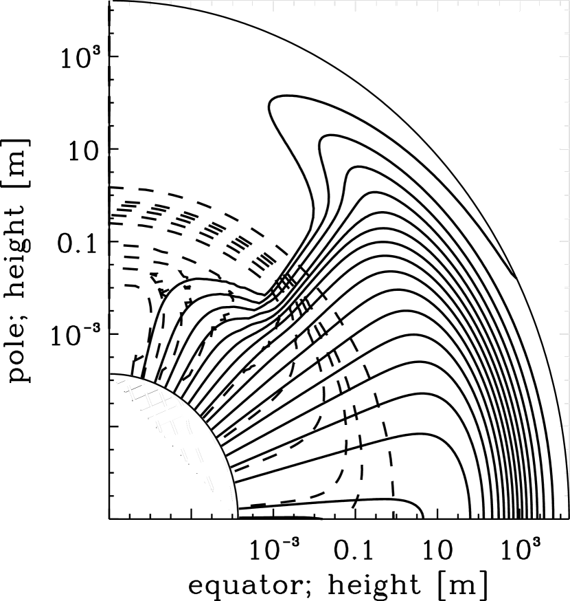
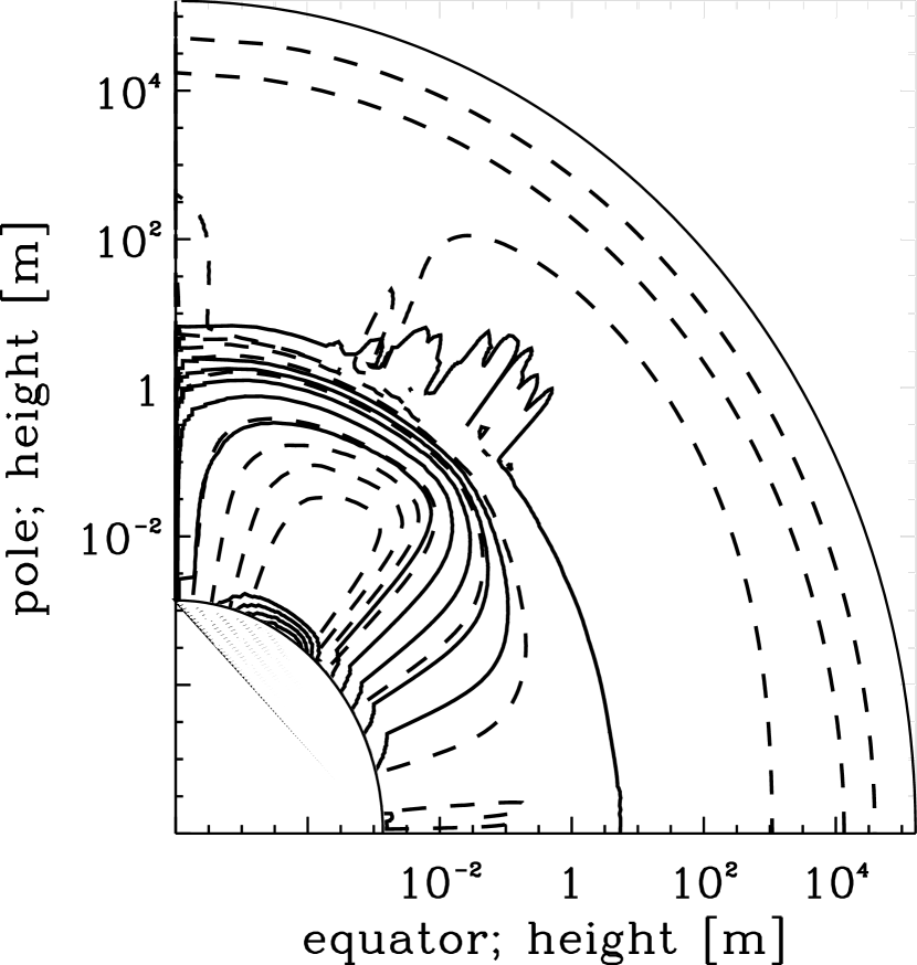
Figure 1: ($a$) Numerical calculation of the hydromagnetic structure of the accreted layer, showing contours of $\psi$ (solid) and $\rho$ (dashed). ($b$) Contours of Lorentz force density (solid) and magnetic field intensity (dashed). Parameters: $M_{\rm a}=10^{-5}M_{\sun}$, $b=10$. The contours are at fractions $\eta=0.8$, 0.6, 0.4, 0.2, $10^{-2}$, $10^{-3}$, $10^{-4}$, $10^{-5}$, $10^{-6}$, and $10^{-12}$ of the respective maxima.

Figure 1$a$ depicts the density profile of the polar mountain (dashed $\rho$ contours) and the flaring geometry of the magnetic field (solid $\psi$ contours), for $M_{\rm a}=10^{-5}M_{\sun}$ and $\psi_{\rm a}/\psi_{\ast}=10^{-1}$. The accreted material spreads equatorward under its own weight until its advance is halted near the equator by the stress of the compressed (and hence amplified, by flux conservation) magnetic field. Figure 1$b$ illustrates this balance of forces; the Lorentz force per unit volume, $(4\pi)^{-1}(\nabla\times{\bf B})\times{\bf B}$ (solid contours), peaks at the boundary $\psi_{\rm a}$ of the polar flux tube that receives accreted material, while the local magnetic field intensity, $|{\bf B}|$ (dashed contours), is amplified $\approx 4\times 10^{3}$ times above its initial polar value.

In Figure 2$a$, we plot the gravitational ellipticity $\epsilon=|I_{1}-I_{3}|/I_{1}$, where $I_{1}$ and $I_{3}$ denote principal moments of inertia, as a function of $M_{\rm a}$ for several values of $\psi_{\rm a}/\psi_{\ast}$. The reduced mass quadrupole moment is then given by $2\epsilon I_{zz}/3$, with $I_{zz}\approx 0.4M_{\ast}R_{\ast}^{2}$ (Shapiro & Teukolsky, 1983; Bonazzola & Gourgoulhon, 1996). There is good agreement between the numerical and analytic results for $\psi_{\rm a}/\psi_{\ast}=0.3$, where the gradients are manageable and the code converges reliably. The analytic results follow from a Green function analysis in the small-$M_{\rm a}$ limit, where the source term on the right-hand side of (2) is evaluated for a dipole, yielding (Payne & Melatos, 2004)

$$\psi(x,y)=\psi_{\ast}(1-y^{2})(1+x/a)^{-1}[1-(M_{\rm a}/M_{\rm c})b^{2}yg(y)f(x)]~{},$$ (5)

$$\rho(x,y) = M_{\rm a}ab[2\pi R_{\ast}^{3}f(b)]^{-1}[y^{2}+(1-y^{2})(M_{\rm a}/M_{\rm c})b^{2}yg(y)f(x)]^{1/2}$$

$$\times\exp[-b(1-y^{2})-x+(M_{\rm a}/M_{\rm c})b^{3}yg(y)f(x)]~{},$$

$$\mu=\psi_{\ast}R_{\ast}(1+3M_{\rm a}/4M_{\rm c})^{-1}~{},$$ (7)

$$\epsilon=(5M_{\rm a}/2M_{\ast})(1-3/2b)(1+M_{\rm a}b^{2}/8M_{\rm c})^{-1}~{},$$ (8)

to leading order in $M_{\rm a}/M_{\rm c}$, with

$$M_{\rm c}=GM_{\ast}\psi_{\ast}^{2}/4c_{\rm s}^{4}R_{\ast}^{2}~{}.$$ (9)

We define the dimensionless quantities $x=a(r/R_{\ast}-1)$, $y=\cos\theta$, $f(x)=1-\exp(-x)$, $g(y)=\exp[-b(1-y^{2})]$, $a=GM_{\ast}/c_{\rm s}^{2}R_{\ast}$, and $b=\psi_{\ast}/\psi_{\rm a}$. Typically, the hydrostatic scale height is small compared to $R_{\ast}$, as is the polar fraction of the hemispheric flux, implying $a\gg 1$ and $b\gg 1$ respectively. The critical accreted mass $M_{\rm c}$ depends on the natal magnetic flux and crustal temperature through (9), with $M_{\rm c}/M_{\sun}=3\times 10^{-4}(\psi_{\ast}/10^{24}\,{\rm G\,cm^{2}})^{2}(T/10^{8}\,{\rm K})^{-2}$.

The $\epsilon$($M_{\rm a}$) relation (8) associated with magnetic burial is new, while the $\mu$($M_{\rm a}$) relation (7) is closely related to the phenomenological scaling invoked by Shibazaki et al. (1989) to model observations of binary and millisecond radio pulsars (Taam & van de Heuvel, 1986; van den Heuvel & Bitzaraki, 1995). It is important to note that magnetic burial affects $\epsilon$ and $\mu$ in different ways. The accreted mass above which $\epsilon$ saturates, $8M_{\rm c}b^{-2}$, and the saturation ellipticity, $\epsilon_{\rm max}=20(M_{\rm c}/M_{\ast})b^{-2}(1-3/2b)$, are inversely proportional to $b^{2}$ (for $b\gg 1$), whereas the accreted mass above which $\mu$ is screened, $4M_{\rm c}/3$, is independent of $b$. This theoretical prediction conforms with observations in two key respects. First, most accreting millisecond pulsars have $b\gtrsim 10$ (Litwin et al., 2001) and hence $\epsilon_{\rm max}\lesssim 10^{-7}$ from (8), consistent with the upper limit $\epsilon\lesssim 10^{-5}$ inferred from spin down (Dhurandhar et al., 1996; Brady et al., 1998) and the failure of bar antennas and interferometers to detect gravitational waves so far (Schutz, 1999). Contours of $\epsilon_{\rm max}$ are plotted in the $\psi_{\ast}$-$T$ plane in Figure 2$b$. Second, the floor magnetic moment of recycled neutron stars, which is observed to be ‘universal’, is given by $\mu_{\rm min}\sim 10^{26}\,{\rm G\,cm^{-3}}$ (for $M_{\rm a}\sim 10^{-1}M_{\sun}$) from (7). Theoretically, it is independent of $b$ (and hence $\dot{M}_{\rm a}$) in the regime $t_{\rm d}\gtrsim t_{\rm a}$, and weakly dependent on $\dot{M}_{\rm a}$ in the regime $t_{\rm d}\lesssim t_{\rm a}$ (Shibazaki et al., 1989; Melatos & Phinney, 2001).

The dipole and quadrupole moments saturate at $\mu(M_{\rm d})$ and $\epsilon(M_{\rm d})$ respectively when Ohmic diffusion dominates ($M_{\rm a}>M_{\rm d}$; see §2.2). From (4), (5), and (9), we obtain

$$\frac{M_{\rm d}}{M_{\sun}}=3.4\times 10^{-7}Z^{-4/9}\left(\frac{\psi_{\rm a}}{0.1\psi_{\ast}}\right)^{16/9}\left(\frac{T}{10^{8}\,{\rm K}}\right)^{-20/9}\left(\frac{\psi_{\ast}}{10^{24}\,{\rm G\,cm^{2}}}\right)^{16/9}\left(\frac{\dot{M}_{\rm a}}{\dot{M}_{\rm Edd}}\right)^{4/9}.$$ (10)

Contours of $M_{\rm d}$ in the $\dot{M}_{\rm a}$-$T$ plane are displayed in Figure 3.

The distorted magnetic field in Figure 1$a$ may be disrupted by interchange, Parker, and doubly diffusive instabilities wherever the local field strength exceeds $B\sim 10^{10}\,{\rm G}$ (Cumming et al., 2001; Litwin et al., 2001; Payne & Melatos, 2004). However, more work is required to settle this issue; existing stability calculations are linear and plane-parallel, unlike the situation in Figure 1$a$. The equilibrium field may not be disrupted completely if the instability saturates promptly in the nonlinear regime; for example, the interchange instability is inhibited topologically by the line-tying boundary condition, which constrains the mobility of closely packed flux tubes. In a separate effect, Payne & Melatos (2004) proved analytically that the magnetic field develops bubbles for $M_{\rm a}\gtrsim 10^{-4}M_{\sun}$; the source term on the right-hand side of (2) creates flux surfaces $\propto F^{\prime}(\psi)\propto M_{\rm a}$ that are disconnected from the star ($\psi<0$, $\psi>\psi_{\ast}$). Further work is required to determine how the bubbles evolve in the large-$M_{\rm a}$ regime (e.g. $M_{\rm a}\sim 10^{-1}M_{\sun}$), where the theory in §2.1 breaks down.

3 Gravitational radiation

3.1 Detectability

The mass distribution resulting from polar magnetic burial is not rotationally symmetric in general; the principal axis of inertia ${\bf e}_{3}$ (i.e. the dipole axis of the natal magnetic field) is inclined at an angle $\alpha$ to the rotation axis. Gravitational waves are emitted by the deformed star at the spin frequency $\Omega=f/2$ and its first harmonic $2\Omega=f$ (unless $\alpha=\pi/2$, when there is no $f/2$ component), and the spin-down luminosity is proportional to $(16\sin^{2}\alpha+\cos^{2}\alpha)\sin^{2}\alpha$ (Shapiro & Teukolsky, 1983; Bonazzola & Gourgoulhon, 1996). Upon averaging over $\alpha$, polarization, and orientation (the position angle of the rotation axis on the sky cannot normally be measured), one can define the characteristic gravitational wave strain $h_{\rm c}=(128\pi^{4}/15)^{1/2}GI_{zz}f^{2}\epsilon/(dc^{4})$ (Brady et al., 1998), which reduces to

$$h_{\rm c}=7.7\times 10^{-19}\left(\frac{M_{\rm a}}{M_{\ast}}\right)\left(1-\frac{3}{2b}\right)\left(1+\frac{M_{\rm a}b^{2}}{8M_{\rm c}}\right)^{-1}\left(\frac{f}{0.6\,{\rm kHz}}\right)^{2}\left(\frac{d}{1\,{\rm kpc}}\right)^{-1}$$ (11)

upon substituting (8). Polar magnetic burial therefore generates gravitational radiation whose amplitude $h_{\rm c}\approx 6\times 10^{-26}$ (for typical parameters $M_{\rm a}\gtrsim M_{\rm c}\sim 10^{-5}M_{\ast}$ and $b=30$) is $\sim 10^{5}$ times greater than that produced by the natal, undistorted magnetic dipole, $h_{\rm c}\approx 10^{-31}(B/10^{12}\,{\rm G})^{2}(f/0.6\,{\rm kHz})^{2}(d/1\,{\rm kpc})^{-1}$ (Katz, 1989; Bonazzola & Gourgoulhon, 1996), due to the enhanced Maxwell stress from the compressed equatorial magnetic field. The self-consistent form of $F(\psi)$ defined by (3) is needed to calculate this stress properly; cf. Melatos & Phinney (2001).

Figure 4$a$ is a plot of $h_{\rm c}$ versus $f$ for $10^{-8}\leq M_{\rm a}/M_{\sun}\leq 10^{-2}$ and $10\leq b\leq 10^{2}$. The sensitivity curves for initial LIGO ($L$) and advanced LIGO ($AL$) are superimposed, corresponding to the weakest source detectable with 99 per cent confidence in $\tau=10^{7}\,{\rm s}$ of integration time, if the frequency and phase of the signal at the detector are known in advance (Brady et al., 1998; Schutz, 1999). The plot suggests that the prospects of detecting objects with $M_{\rm a}\gtrsim 10^{-5}M_{\sun}$ are encouraging, a point first made in the context of magnetic burial by Melatos & Phinney (2000). Such objects include the five accreting X-ray millisecond pulsars discovered at the time of writing, SAX J1808.4$-$3658, XTE J1751$-$305, XTE J0929$-$314, XTE J1807$-$294, and XTE J1814$-$338 (Wijnands & van der Klis, 1998; Chakrabarty & Morgan, 1998; Galloway et al., 2002; Markwardt et al., 2002; Strohmayer et al., 2003; Campana et al., 2003). Detectability is facilitated if the time-dependent Doppler shift from the binary orbit is known well enough to be subtracted, but this is only practical for some objects of known $f$, not for an all-sky search (Brady et al., 1998).

The characteristic gravitational wave strain $h_{\rm c}$ is a lower limit in an important sense: it contains the assumption that, after averaging over polarization and orientation, the bulk of the gravitational wave signal is emitted at $f=2\Omega$. This is true when the observer views the system along its rotation axis and measures $h^{+}\propto h^{\times}\propto e^{2i\Omega t}\sin^{2}\alpha$ in the two polarizations. It is not true when the observer views the system perpendicular to its rotation axis and measures $h^{+}\propto e^{2i\Omega t}\sin^{2}\alpha$ and $h^{\times}\propto e^{i\Omega t}\sin\alpha\cos\alpha$, for example (Shapiro & Teukolsky, 1983; Bonazzola & Gourgoulhon, 1996). One certainly expects, as a matter of chance, to observe some systems in the latter orientation, or close to it. For these sources, the average quantity $h_{\rm c}$ substantially underestimates the true wave strain (which is dominated by $h^{\times}$ in the above example), especially if $\alpha$ is small. (The observed pulse modulation indices of accreting millisecond pulsars imply a range of $\alpha$ values.) The effect on detectability is even greater when one takes into account the shape of the interferometer’s noise curve; for example, LIGO is $1.5$–$2.5$ times more sensitive at $\Omega\sim 0.3\,{\rm kHz}$ than at $2\Omega\sim 0.6\,{\rm kHz}$.

3.2 $h_{\rm c}$ versus $\mu$

Polar magnetic burial is not the only mechanism whereby accreting neutron stars with $M_{\rm a}\gtrsim 10^{-5}M_{\sun}$ can act as gravitational wave sources detectable by long baseline interferometers. Crustal deformation due to temperature gradients (§4) is one of several alternatives (Bildsten, 1998; Ushomirsky et al., 2000). In principle, we can distinguish between these mechanisms by eliminating $M_{\rm a}$ from (7) and (8) to derive a unique — and testable — scaling $h_{\rm c}(\mu)$ for magnetic burial that relates observable quantities only, unlike (11), which features $M_{\rm a}$ (usually inferred from evolutionary models) (van den Heuvel & Bitzaraki, 1995). The scaling,

$$h_{\rm c}\propto(1-3/2b)[\mu/(\psi_{\ast}R_{\ast}-\mu)+b^{2}/6]^{-1},$$ (12)

is graphed in Figure 4$b$ for $3\leq b\leq 100$. The vertical segments of all the curves represent the regime $M_{\rm a}\ll M_{\rm c}$, where $\mu$ retains its natal value while the ellipticity grows as $M_{\rm a}$. The horizontal segments represent the regime $M_{\rm a}\gg M_{\rm c}$, where $\epsilon$ saturates while $\mu$ decreases, with the turn-off mass and $\epsilon_{\rm max}$ scaling as $b^{-2}$. The proportionality (12) does depend on $b$ and $\psi_{\ast}$, neither of which can be measured, but the relevant scalings are moderately weak (e.g. $b\propto\dot{M}_{\rm a}^{-2/7}\psi_{\ast}^{4/7}$). Consequently, the overall trend in Figure 4$b$ may emerge statistically, once many gravitational wave sources have been detected, provided that the range of neutron star magnetic fields at birth is relatively narrow. Drawing upon population synthesis simulations, Hartman et al. (1997) inferred that $\approx 90$ per cent of radio pulsars are born with $10^{23.5}\,{\rm G\,cm^{2}}\leq\psi_{\ast}\leq 10^{24.5}\,{\rm G\,cm^{2}}$, but the existence of anomalous X-ray pulsars implies a wider range of $\psi_{\ast}$ in a subset of the neutron star population (Regimbau & de Freitas Pacheco, 2001).

4 Discussion

In this paper, we report on two new results concerning the gravitational radiation emitted by accreting neutron stars undergoing polar magnetic burial. First, upon calculating rigorously the hydromagnetic structure of the polar mountain, by solving a Grad-Shafranov boundary value problem with the correct flux freezing condition connecting the initial and final states, we find that the ellipticity of the star materially exceeds previous estimates, due to the enhanced Maxwell stress exerted by the compressed equatorial magnetic field, with $\epsilon\approx 20M_{\rm c}/M_{\ast}b^{2}$ for $M_{\rm a}\gtrsim M_{\rm c}\sim 10^{-5}M_{\sun}$, as given by (9). The associated gravitational wave strain at Earth, $h_{\rm c}=6\times 10^{-24}(M_{\rm a}/M_{\rm c})(1+M_{\rm a}b^{2}/8M_{\rm c})^{-1}(f/0.6\,{\rm kHz})^{2}(d/1\,{\rm kpc})^{-1}$, averaged over polarization and orientation, is detectable in principle by the current generation of long baseline interferometers, e.g. LIGO. (The wave strain at $f/2=\Omega$ in one polarization can exceed $h_{\rm c}$ for many orientations and $\alpha$ values.) Second, the stellar magnetic moment $\mu$ decreases as the polar mountain grows and spreads equatorward, implying a distinctive, observable scaling $h_{\rm c}(\mu)$, displayed in Figure 4$b$, which can be used to test the magnetic burial hypothesis. Accreting neutron stars are easier to detect as gravitational wave sources than other kilohertz sources like coalescing neutron star binaries: they are persistent rather than transient, the waveform is approximately sinusoidal, and, if X-ray pulsations or thermonuclear burst oscillations are observed in advance (e.g. SAX J1808.4$-$3658), extra sensitivity can be achieved by integrating coherently.

The range of $\epsilon$ predicted by the theory of magnetic burial is consistent with that invoked by Bildsten (1998) to explain the clustering of spin frequencies (within 40 per cent of $0.45\,{\rm kHz}$) of weakly magnetized, accreting neutron stars (Chakrabarty et al., 2003) in terms of a stalling effect where the gravitational wave torque ($\propto\Omega^{5}$) balances the accretion torque ($\propto\dot{M}_{\rm a}R_{\rm a}^{1/2}\propto\dot{M}_{\rm a}^{6/7}\mu^{2/7}$). Importantly, the theory of magnetic burial predicts that $\epsilon$ increases monotonically with $M_{\rm a}$ — a key precondition for the stalling effect to operate properly, otherwise the stall frequency $\Omega$ would not be a stable fixed point. In an alternative scenario, Bildsten (1998) and Ushomirsky et al. (2000) attribute the requisite mass quadrupole moment, $2\times 10^{-7}I_{zz}(\dot{M}_{\rm a}/\dot{M}_{\rm Edd})^{1/2}(f/0.6\,{\rm kHz})^{-5/2}$, to lateral temperature gradients in the outer crust, which induce gradients in the electron capture rate and hence $\rho$.

Magnetic burial, acting in concert with the stalling effect, influences the rotational evolution of an accreting neutron star in two observationally testable ways. First, during the late stages of accretion, the instantaneous net torque is zero, because the gravitational wave and accretion torques balance (Bildsten, 1998), but the average torque (on the time-scale $t_{\rm a}$) is effectively negative, because the gravitational wave torque increases with $M_{\rm a}$ as the polar mountain grows; that is, the instantaneous stall frequency $\Omega\propto\dot{M}_{\rm a}^{6/35}\mu(M_{\rm a})^{2/35}\epsilon(M_{\rm a})^{-2/5}$ decreases with $M_{\rm a}$. This effect ought to be detectable by X-ray timing experiments in progress (Galloway et al., 2002), although it may be masked if $\dot{M}_{\rm a}$ fluctuates stochastically on the time-scale $t_{\rm a}$, as commonly happens. Second, magnetic burial predicts a distinctive evolutionary relation between $\mu$ and $\Omega$. During the early stages of accretion, before the star is spun up to the stall frequency, $\Omega$ increases while $\mu$ decreases due to burial, with $\Omega\propto R_{\rm a}^{1/2}M_{\rm a}\propto\dot{M}_{\rm a}^{-1/7}\mu^{-5/7}$ in the regime $\mu\propto M_{\rm a}^{-1}$. However, during the late stages of accretion, $\Omega$ and $\mu$ both decrease as explained above. Hence there exists a maximum spin frequency $\Omega/2\pi\lesssim 1\,{\rm kHz}$ bounding the population of accreting millisecond pulsars in the $\Omega$-$\mu$ plane, and objects follow $\Lambda$-shaped evolutionary tracks in that plane.

Once accretion ends, do we expect to detect the neutron star as a radio millisecond pulsar? There are two arguments against this from the perspective of magnetic burial. First, the gravitational wave spin-down time, $t_{\rm g}\approx 5\times 10^{7}(\epsilon/10^{-7})^{-2}(\Omega/2\,{\rm krad\,s^{-1}})^{-4}\,{\rm yr}$, is shorter than the observed age, so the neutron star rapidly brakes below the radio pulsar death line ($\Omega/2\pi<0.1\,{\rm kHz}$) and is extinguished as a radio source. Note that this occurs no matter what generates the quadrupole moment inferred from the stalling effect. Second, this rapid spin-down is interrupted if the stellar deformation relaxes quickly (compared to $t_{\rm g}$), for example if the buried, polar magnetic field is resurrected on the Ohmic time-scale $t_{\rm d}$ of the outer crust, which satisfies $t_{\rm d}\sim t_{\rm a}=6\times 10^{7}(M_{\rm a}/M_{\sun})(\dot{M}_{\rm a}/\dot{M}_{\rm Edd})^{-1}\,{\rm yr}$ in the regime $M_{\rm a}\gtrsim 10^{-5}M_{\sun}$. However, the buried field is resurrected in stages; the steepest gradients are smoothed out ($L\propto t_{\rm a}^{1/2}$), but the natal field is not fully restored over the typical lifetime of a millisecond pulsar, because one has $\mu\propto L\propto t_{\rm a}^{1/2}$ and hence $B\sim 10^{9-10}\,{\rm G}$ after $\sim 10^{9}\,{\rm yr}$ (Cumming et al., 2001; Melatos & Phinney, 2001). This scenario leaves the radio millisecond pulsars with the lowest fields unexplained unless they have low fields initially.

Figure 2: ($a$) Ellipticity $\epsilon=|I_{1}-I_{3}|/I_{1}$ as a function of accreted mass $M_{\rm a}$, for $b=\psi_{\ast}/\psi_{\rm a}=3$, $10$, $30$, $100$. The curves are theoretical, based on the expressions (5)–(9). The points are numerical results for $b=3$. Parameters: $\psi_{\ast}=10^{24}\,{\rm G\,cm^{2}}$, $T=10^{8}\,{\rm K}$. ($b$) Contours of maximum ellipticity $\epsilon_{\rm max}=20M_{\rm c}/(M_{\ast}b^{2})$, from (7) and (9), as a function of total magnetic flux $\psi_{\ast}$ and crustal temperature $T$. Contours are spaced logarithmically in the range $10^{-9}\leq M_{\rm c}/M_{\sun}\leq 10^{-4}$. In both panels, the regime $t_{\rm d}>t_{\rm a}$ is considered to highlight the effects of burial in isolation.

Figure 3: Contours of $M_{\rm d}$, the minimum accreted mass for which Ohmic diffusion arrests the growth of the polar mountain ($t_{\rm d}\leq t_{\rm a}$). The plot shows the variation of $M_{\rm d}$ with accretion rate $\dot{M}_{\rm a}$ (in units of $\dot{M}_{\rm Edd}$) and crustal temperature $T$ (in kelvins), in the range $10^{-8}\leq M_{\rm d}/M_{\sun}\leq 10^{-5}$, with $\psi_{\rm a}/\psi_{\ast}=0.1$, $Z=1$, and $\psi_{\ast}=10^{24}\,{\rm G\,cm^{2}}$. $M_{\rm d}$ is calculated from (4), (5), and (9).

Figure 4: ($a$) Polarization- and orientation-averaged gravitational wave strain $h_{\rm c}$ as a function of wave frequency $f$. The initial and advanced LIGO noise curves (solid) correspond to detection with 99 per cent confidence after $10^{7}\,{\rm s}$ of coherent integration (Schutz, 1999). Theoretical curves are shown for $b=10$, $M_{\rm a}/M_{\sun}=10^{-2}$, $10^{-4}$, $10^{-6}$ (dashed, top to bottom) and $b=10^{2}$, $M_{\rm a}/M_{\sun}=10^{-4}$, $10^{-8}$ (dotted, top to bottom). ($b$) Gravitational wave strain $h_{\rm c}$ versus magnetic moment $\mu$ (scaled to the natal magnetic moment $\mu_{\rm i}=\psi_{\ast}R_{\ast}$) for $b=3$, 10, $30$, $100$, from (7) and (8).

References

- Andersson (1998) Andersson, N. 1998, ApJ, 502, 708
- Bildsten (1998) Bildsten, L. 1998, ApJ, 501, L89+
- Bonazzola & Gourgoulhon (1996) Bonazzola, S., & Gourgoulhon, E. 1996, A&A, 312, 675
- Brady & Creighton (2000) Brady, P. R., & Creighton, T. 2000, Phys. Rev. D, 61, 82001
- Brady et al. (1998) Brady, P. R., Creighton, T., Cutler, C., & Schutz, B. F. 1998, Phys. Rev. D, 57, 2101
- Brown & Bildsten (1998) Brown, E. F., & Bildsten, L. 1998, ApJ, 496, 915
- Campana et al. (2003) Campana, S., Ravasio, M., Israel, G. L., Mangano, V., & Belloni, T. 2003, ApJ, 594, L39
- Chakrabarty & Morgan (1998) Chakrabarty, D., & Morgan, E. H. 1998, Nature, 394, 346
- Chakrabarty et al. (2003) Chakrabarty, D., Morgan, E. H., Muno, M. P., Galloway, D. K., Wijnands, R., van der Klis, M., & Markwardt, C. B. 2003, Nature, 424, 42
- Cumming (2002) Cumming, A. 2002, MNRAS, 333, 589
- Cumming et al. (2004) Cumming, A., Arras, P., & Zweibel, E. 2004, ApJ, 609, 999
- Cumming et al. (2001) Cumming, A., Zweibel, E., & Bildsten, L. 2001, ApJ, 557, 958
- Cutler (2002) Cutler, C. 2002, Phys. Rev. D, 66, 84025
- Dhurandhar et al. (1996) Dhurandhar, S. V., Blair, D. G., & Costa, M. E. 1996, A&A, 311, 1043
- Galloway et al. (2002) Galloway, D. K., Chakrabarty, D., Morgan, E. H., & Remillard, R. A. 2002, ApJ, 576, L137
- Geppert & Urpin (1994) Geppert, U., & Urpin, V. 1994, MNRAS, 271, 490
- Hameury et al. (1983) Hameury, J. M., Bonazzola, S., Heyvaerts, J., & Lasota, J. P. 1983, A&A, 128, 369
- Hartman et al. (1997) Hartman, J. W., Bhattacharya, D., Wijers, R., & Verbunt, F. 1997, A&A, 322, 477
- Heyl (2000) Heyl, J. S. 2000, MNRAS, 317, 310
- Ioka (2001) Ioka, K. 2001, MNRAS, 327, 639
- Jones (1975) Jones, P. B. 1975, Ap&SS, 33, 215
- Katz (1989) Katz, J. I. 1989, MNRAS, 239, 751
- Konno et al. (2000) Konno, K., Obata, T., & Kojima, Y. 2000, A&A, 356, 234
- Lindblom et al. (1998) Lindblom, L., Owen, B. J., & Morsink, S. M. 1998, Physical Review Letters, 80, 4843
- Link & Epstein (2001) Link, B., & Epstein, R. I. 2001, ApJ, 556, 392
- Litwin et al. (2001) Litwin, C., Brown, E. F., & Rosner, R. 2001, ApJ, 553, 788
- Markwardt et al. (2002) Markwardt, C. B., Swank, J. H., Strohmayer, T. E., Zand, J. J. M. i., & Marshall, F. E. 2002, ApJ, 575, L21
- Melatos & Phinney (2000) Melatos, A., & Phinney, E. S. 2000, in ASP Conf. Ser. 202: IAU Colloq. 177: Pulsar Astronomy - 2000 and Beyond, 651–+
- Melatos & Phinney (2001) Melatos, A., & Phinney, E. S. 2001, Publications of the Astronomical Society of Australia, 18, 421
- Mouschovias (1974) Mouschovias, T. C. 1974, ApJ, 192, 37
- Palomba (2001) Palomba, C. 2001, A&A, 367, 525
- Payne & Melatos (2004) Payne, D. J. B., & Melatos, A. 2004, MNRAS, 351, 569
- Phinney (1991) Phinney, E. S. 1991, ApJ, 380, L17
- Regimbau & de Freitas Pacheco (2001) Regimbau, T., & de Freitas Pacheco, J. A. 2001, A&A, 374, 182
- Schutz (1999) Schutz, B. F. 1999, Classical and Quantum Gravity, 16, A131
- Shapiro & Teukolsky (1983) Shapiro, S. L., & Teukolsky, S. A. 1983, Black holes, white dwarfs, and neutron stars: The physics of compact objects (Research supported by the National Science Foundation. New York, Wiley-Interscience, 1983, 663 p.)
- Shibazaki et al. (1989) Shibazaki, N., Murakami, T., Shaham, J., & Nomoto, K. 1989, Nature, 342, 656
- Strohmayer et al. (2003) Strohmayer, T. E., Markwardt, C. B., Swank, J. H., & in’t Zand, J. 2003, ApJ, 596, L67
- Taam & van de Heuvel (1986) Taam, R. E., & van de Heuvel, E. P. J. 1986, ApJ, 305, 235
- Uchida & Low (1981) Uchida, Y., & Low, B. C. 1981, Journal of Astrophysics and Astronomy, 2, 405
- Ushomirsky et al. (2000) Ushomirsky, G., Cutler, C., & Bildsten, L. 2000, MNRAS, 319, 902
- van den Heuvel & Bitzaraki (1995) van den Heuvel, E. P. J., & Bitzaraki, O. 1995, A&A, 297, L41+
- Wijnands & van der Klis (1998) Wijnands, R., & van der Klis, M. 1998, Nature, 394, 344