Measuring the Galaxy-Galaxy-Mass Three-point Correlation Function with Weak Gravitational Lensing

Abstract

We discuss the galaxy-galaxy-mass three-point correlation function and show how to measure it with weak gravitational lensing. The method entails choosing a large of pairs of foreground lens galaxies and constructing a mean shear map with respect to their axis, by averaging the ellipticities of background source galaxies. An average mass map can be reconstructed from this shear map and this will represent the average mass distribution around pairs of galaxies. We show how this mass map is related to the projected galaxy-galaxy-mass three-point correlation function. Using a large N-body dark matter simulation populated with galaxies using the Halo Occupation Distribution (HOD) bias prescription, we compute these correlation functions, mass maps, and shear maps. The resultant mass maps are distinctly bimodal, tracing the galaxy centers and remaining anisotropic up to scales much larger than the galaxy separation. At larger scales, the shear is approximately tangential about the center of the pair but with small azimuthal variation in amplitude. We estimate the signal-to-noise ratio of the reconstructed mass maps for a survey of similar depth to the Sloan Digital Sky Survey (SDSS) and conclude that the galaxy-galaxy-mass three-point function should be measurable with the current SDSS weak lensing data. Measurements of this three-point function, along with galaxy-galaxy lensing and galaxy auto-correlation functions, will provide new constraints on galaxy bias models. The anisotropic shear profile around close pairs of galaxies is a prediction of cold dark matter models and may be difficult to reconcile with alternative theories of gravity without dark matter.

1 Introduction

The last few years have seen the emergence of an observationally consistent cosmological model based on firm physical ideas. The hot big bang model of the expanding universe, whose structure and dynamics can be described by general relativity (GR), has a number of cosmological parameters that are now well constrained by numerous observations. WMAP measurements of the cosmic microwave background radiation (CMB) (Spergel et al., 2003), supernova measurements (Riess et al., 1998; Perlmutter et al., 1999), and measurements of large scale structure (Tegmark et al., 2003) among others, have settled on a concordance model of a spatially flat universe with matter density about 25% of critical. This concordance model is consistent with the ages of the oldest stars (Jimenez et al., 1996), Hubble parameter measurements (Freedman et al., 2001), and primordial abundances of light elements from Big Bang Nucleosynthesis (BBN) (Burles et al., 2001).

One of the main requirements of a successful cosmological model is that it connect measurements of the early universe, e.g. the CMB and BBN, to the measurements of the local universe of galaxies and stars. The large scale structure of galaxies that we observe in galaxy surveys must have formed through gravitational collapse of the small fluctuations left over from that earlier time. The properties of these large-scale mass densities can be predicted from the initial conditions as observed in the CMB combined with our understanding of gravity as described by general relativity. However, since the Universe in our model is dominated by dark matter, we need to make the connection between the distribution of galaxies relative to the dark matter if we want to compare these observed structures to what is predicted.

The relation between the galaxy density and the dark matter density is known as the bias. For the concordance model to be in agreement with the data on galaxy clustering, it is required that on large scales the bias parameter (which we will define shortly) is close to one. On smaller scales the bias must be different from one but of order unity. Moreover, the relative bias of different galaxy types is known to depend on spectral type and luminosity. One can do better than simply treating the bias as a free parameter. Galaxy biasing is after all closely linked to the physics of galaxy formation. Although galaxy formation is not completely understood, it is becoming increasingly amenable to theoretical modeling and numerical simulation. Gas dynamical N-body simulations and Semi-analytic models of galaxy formation (Benson et al., 2000; Kauffmann et al., 1999) each predict how galaxies are biased with respect to mass. Nevertheless, sufficient uncertainty on the details of galaxy formation remain that observational constraints on the bias are needed.

The apparent complexity of the bias has motivated the development of new probes of large-scale structure and bias that do not rely on luminous galaxies as tracers of the underlying mass. Gravitational lensing is a prime example. Lensing is ideally suited to studying dark matter since it is directly sensitive to the total mass density along the line of sight. Other probes of dark matter such as dynamical measurements must rely on some assumptions such as that a system has reached dynamical equilibrium. By contrast, lensing provides a clean probe of the dark matter.

Galaxy-galaxy lensing (GGL), in particular, probes the dark matter density profile around luminous galaxies. In galaxy-galaxy lensing, one measures the mean tangential distortion of a large number of source galaxies behind foreground lens galaxies by stacking the signal from the latter (Sheldon et al., 2004). To date, lensing measurements and theory have focused on the two-point galaxy-mass correlation function (2PCF). This correlation function can be measured from galaxy photometric surveys and compared to the results of N-body dark matter simulations. These measurements provide direct constraints on bias models. Although they do not measure the galaxy bias parameter, $b$ , directly, they do measure a closely related quantity and so these measurements do test the bias model.

While the 2PCF is the lowest order measurement of how much a distribution is clustered, it does not carry complete statistical information about a non-Gaussian distribution. The rest of the information is encoded in the infinite set of N-point correlation functions. In particular the higher order ($\mbox{N}>2$) functions provide the information about the coherence and shapes of large-scale structures such as filaments, walls, and voids that are apparent in both data and simulations. These higher order correlation functions add further constraints to be met by cold dark matter (CDM) models and new probes of the bias.

For the most part observational studies of higher order correlation functions have measured correlations between galaxies. In this paper we will describe a method for measuring the galaxy-galaxy-mass three-point correlation function (GGM3PCF) with weak lensing. This method is a generalization of the method for measuring the galaxy-mass two-point correlation function (GM2PCF) with galaxy-galaxy lensing. Just as the GM2PCF provided new constraints on the bias model, so too does the GGM3PCF. While the GM2PCF is a measure of the isotropic mass density around galaxies, the GGM3PCF gives us information about the shape of the mass distribution around pairs of galaxies. Together with galaxy N-point functions and the GM2PCF, the GGM3PCF provides independent constraints on models of galaxy biasing that are crucial for understanding both large scale structure and the processes of galaxy formation.

It is reasonable to assume that CDM models should predict that the mass around a pair of galaxies will have an anisotropic distribution. A priori it may be purely elliptical or clumped tightly about each galaxy with a distinctly bimodal appearance. This expectation comes from the fact that halos are not themeselves spherically symmetic and that the galaxies should also trace this ellipticity. Also the galaxies themselevs have mass associates with them; stellar mass at the least and probably dark matter sub-halos. Whatever the details of the distribution is, it will create a gravitational lensing effect that is also anisotropic. This anisotropic lensing signal should be measurable with current and future weak lensing surveys.

Another use of the GGM3PCF is to test for the existence of dark matter itself. Alternative theories of gravity with no dark matter, e.g. MOND (Milgrom, 1983), must eventually make prediction for gravitational lensing. This predicted lensing profile must agree with the lensing observations. With no dark matter, the lensing effect is only caused by the visible matter. Two galaxies that are close together will simply look like a monopole at large distance from them and the lensing effect produced should be nearly isotropic regardless of the form of the lensing profile. However, dark matter models predict (as we will demonstrate) that galaxy pairs have an extended dark matter halo about them that is anisotropic even at large distance from their center. This causes an anisotropic lensing effect at these large distances. Thus, dark matter models and alternative models should make different predictions for the lensing anisotropy and thus test the idea of the existence of dark matter. Hoekstra et al. 2003 have already claimed to have measured halo flattening around single galaxies, a similar effect, with weak lensing and argue that it would be difficult to reconcile this anisotropy with theories such as MOND. Measurements of the GGM3PCF would allow one to extend this result to scales larger than the size of individual galaxies. Also, since the GGM3PCF deals with only the locations of galaxies, it would not have to rely on simulations that predict how the shape of the galaxy light correlates with the shape of the halo.

In this paper, we show how the lensing pattern around pairs of galaxies is related to the GGM3PCF. In particular, we show how the 2D projection of the 3D GGM3PCF is directly measurable with weak lensing measurements such as the measurements being conducted (Sheldon et al., 2004; McKay et al., 2001) with data from the Sloan Digital Sky Survey (York & SDSS collaboration, 2000). We use an N-body dark matter simulation populated with galaxies using a bias model chosen to reproduce the results of the hydrodynamical simulations and make numerical calculations of the various two and three-point correlation functions in both 2D and 3D. We calculate the lensing effect and estimate the amount of noise that should be present to study the signal-to-noise that can be obtained. We conclude that the GGM3PCF can now be measured with the present SDSS data.

2 Correlation Functions and their Applications to Cosmology

We begin by reviewing galaxy correlation functions and then describe their extension to galaxy-mass cross-correlations. The probability of finding a galaxy (or any mass point) in an infinitesimal volume of space $dV_{1}$ is simply $dP_{g}=\rho_{g}dV_{1}$ where $\rho_{g}$ is the mean galaxy density. The probability of finding one galaxy in $dV_{1}$ and another in $dV_{2}$ defines the two-point correlation function $\xi_{gg}(r)$

$$dP_{gg}=\rho_{g}^{2}dV_{1}dV_{2}~{}[1+\xi_{gg}(r)]$$

The function $\xi_{gg}(r)$ can be thought of as the contribution of clustering to the joint probability in excess of random. By the assumed large scale homogeneity and isotropy, $\xi_{gg}$ can depend only on $r$ and not on angle or location in space. The marginal probability of finding a galaxy in $dV_{2}$ given that one already has found one in $dV_{1}$ is $dP(g_{2}|g_{1})=\rho_{g}^{2}dV_{1}dV_{2}~{}[1+\xi_{gg}(r)]/\rho_{g}dV_{1}=\rho_{g}dV_{2}~{}[1+\xi_{gg}(r)]$.

We can further consider the probability of finding a third galaxy in infinitesimal volume $dV_{3}$ in addition to the two in $dV_{1}$ and $dV_{2}$. The resulting joint probability defines the three-point correlation function (3PCF), $\zeta_{ggg}$ ,

$$dP_{ggg}=\rho_{g}^{3}dV_{1}dV_{2}dV_{3}~{}\left[~{}1+\xi_{gg}(r_{12})+\xi_{gg}(r_{13})+\xi_{gg}(r_{23})+\zeta_{ggg}\right]$$

Here $r_{ij}$ refers to the separation between galaxies $i$ and $j$. The point of defining $\zeta_{ggg}$ so as to result in a 5-term expression is similar to the reason we defined a 2-term expression for the 2-point case. If the third galaxy were simply put down at random or not clustered with the first two, or very far from the first two, we would have $dP_{ggg}=\rho_{g}^{3}dV_{1}dV_{2}dV_{3}[1+\xi_{gg}(r_{12})]$. Thus the other three terms, $\xi_{gg}(r_{13})$, $\xi_{gg}(r_{23})$, and $\zeta_{ggg}$, only contribute the excess over this random occurrence and by symmetry of this argument we also get the next two terms $\xi_{gg}(r_{13})$ and $\xi_{gg}(r_{23})$ . The last term $\zeta_{ggg}$ is needed since there is no reason to assume that the first four terms completely describe the joint probability.

The volume averages of the 2PCF, 3PCF, and higher order correlation functions are the moments of the probability distribution of the smoothed density field, e.g. the variance, skewness, kurtosis etc. Since a Gaussian distribution is characterized just by its 2PCF, the 3PCF is the lowest-order N-point statistic that characterizes non-Gaussianity of the density field. Generally non-linear gravitational effects generate a non-Gaussian density distribution even if the initial density field is Gaussian.

One can write down expressions for the joint probabilities of still more galaxies and these in turn will define the N-point correlation functions. The 3PCF $\zeta_{ggg}$, due to the large scale homogeneity and isotropy, is only a function of the three triangle sides $r_{12}$,$r_{13}$, $r_{23}$ (or any other parametrization of the triangle).

One can also define cross correlation functions between different species of objects, for example, between galaxies and dark matter mass particles. We can write down joint probabilities of finding a galaxy and a mass particle, a galaxy and two mass particles, and two galaxies and a mass particle respectively (taking all the $dV$ to be equal in size for simplicity),

$$dP_{gm}= \rho_{g}\rho_{m}dV^{2} [1+\xi_{gm}(r)]$$ (1)

$$dP_{gmm}= \rho_{g}\rho_{m}^{2}dV^{3} [1+\xi_{gm}(r_{g,m_{1}})+\xi_{gm}(r_{g,m_{2}})+\xi_{mm}(r_{m_{1},m_{2}})+\zeta_{gmm}]$$ (2)

$$dP_{ggm}= \rho_{g}^{2}\rho_{m}dV^{3} [1+\xi_{gg}(r_{g_{1},g_{2}})+\xi_{gm}(r_{g_{1},m})+\xi_{gm}(r_{g_{2},m})+\zeta_{ggm}]$$ (3)

These joint probabilities define the three two-point functions, $\xi_{gg}$ , $\xi_{gm}$, $\xi_{mm}$ and the four three-point functions $\zeta_{ggg}$ , $\zeta_{ggm}$, $\zeta_{gmm}$ and $\zeta_{mmm}$.

One can also make the same definitions in 2D for a set of points that have been projected over the third dimension. In this case we will refer to these 2D correlation functions as, for example, $w_{gm}$ for the two-point and $z_{ggm}$ for the three-point functions.

The uses of correlation functions in cosmology are many. In the inflation scenario, structure formation is seeded by random quantum fluctuations. In most models these initial fluctuations are predicted to be Gaussian distributed and therefore completely described by their two-point correlation $\xi(r)$ or its Fourier transform the power spectrum $P(k)$. In this scenario, the 3PCF and higher order correlation functions that arise are entirely due to the onset of non-linear gravitational collapse and so should be predictable with dark matter simulations given a set of cosmological parameters and a galaxy bias prescription.

The first measurements of the galaxy two-point correlation function (Totsuji & Kihara, 1969; Peebles, 1974a; Groth & Peebles, 1977; Gott & Turner, 1979) found that it was well described by a power law, $\xi_{gg}(r)=(r/r_{0})^{-\gamma}$, with $\gamma=1.8$ and $r_{0}\approx 5h^{-1}$ Mpc. The most recent measurements (Zehavi et al., 2003) are now sensitive enough to detect small deviations from a power law, in agreement with predictions that use N-body simulation combined with HOD bias models (see Section 6).

The first measurement of the 3PCF for galaxies was by Peebles & Groth (1975). For these early correlation function measurements, there was no redshift information, so these were measured in terms of angular coordinates $\theta_{12}$ rather than physical length scales $r_{12}$. Constraints on the 3D 2PCF and 3PCF came from inverting the projections. From this first measurement, it was found that to experimental accuracy the 3PCF could be written in a reduced form relating it to the 2PCFs (on scales less than a few Mpcs) as

$$z_{ggg}=~{}Q~{}[w_{gg}(\theta_{12})w_{gg}(\theta_{13})+w_{gg}(\theta_{12})w_{gg}(\theta_{23})+w_{gg}(\theta_{13})w_{gg}(\theta_{23})]$$ (4)

with Q being a constant $\approx 1$. This scaling relation is referred to as hierarchical scaling. Although much effort has gone into deriving such an equation from first principles, no one has shown analytically why this form should be true. However N-body simulations do indicate that the 3PCF approximately takes this form in the non-linear regime probed by these early measurements. On larger scales ($r>10h^{-1}$ Mpcs) where one can treat gravity perturbatively, this factor Q is indeed independent of scale however there is a non-vanishing dependence on triangle shape (Fry, 1984). This large scale shape dependence is a quantitative statement that co-linear triangles or filamentary structures are more likely than isosceles triangles or isotropic structures and physically relects the fact that gravitational collapse happens anisotropically with velocity flows along density gradients (Bernardeau et al., 2002). A visual inspection of recent N-body simulations (Jenkins et al., 1998; Evrard et al., 2002) as well as real data from galaxy redshift surveys (Huchra et al., 1999; Peacock et al., 2001; Tegmark et al., 2003) show the existence of large-scale filaments on the outskirts of giants voids.

The basic hierarchical scaling of Equation 4 was confirmed by Fry & Seldner (1982) however these early measurements from the Lick galaxy catalog did not extend to large enough scales to reveal the expected configuration-dependent signature from gravitational instability (Fry, 1984). Later results by Frieman & Gaztañaga (1999) using the APM survey data, Scoccimarro et al. (2001a) using the IRAS 1.2 Jy survey and Feldman et al. (2001) using the IRAS PSCz survey were in good agreement with the predictions from the gravitational instability picture and provided new constraints on the bias for these samples.

These studies have had much success at measuring the 2PCF and 3PCF of galaxies. Furthermore N-body simulations have been able to make precise predictions, given the cosmological parameters, of the 2PCF and 3PCF of the mass density. However until recently the galaxy-mass correlation functions have remained unmeasured. The measurements of the 3PCF of galaxies in fact can be used to constrain the large scale bias between galaxies and mass but the smaller scale bias has mostly remained a mystery. The fact that on small scales the observed 2PCF of galaxies and the 2PCF of mass from N-body simulations disagree leads to the requirement that there must be scale dependent bias between galaxies and mass if the CDM framework is correct. Another indicator of this complexity is that different populations of galaxies have different measured correlation functions and therefore are biased differently relative to each other. There is no reason why any particular sample of galaxies should trace the dark matter exactly. Trying to measure and model the bias using galaxy-mass correlations is one of the main goals of galaxy-galaxy lensing and the galaxy-mass 3PCF should help achieve this goal.

3 Measuring Correlation Functions with Weak Lensing

The general relativistic lens equation relates the bending angle of light rays to the mass distribution. In the thin lens approximation the deflection can be computed from the projected surface mass density $\Sigma(x,y)=\int dz\rho(x,y,z)$ where $z$ denotes the coordinate along the line of sight. It is customary make this dimensionless by dividing by the geometric factor $\Sigma_{crit}=c^{2}D_{S}/4\pi GD_{L}D_{LS}$, where the distances are the angular diameter distances to the lens, to the source, and from the lens to the source. This defines a dimensionless 2D mass density, or convergence, $\kappa(x,y)=\Sigma(x,y)/\Sigma_{crit}$. It is useful to define a 2D potential

$$\phi(\vec{x})=\frac{1}{\pi}\int d^{2}x^{\prime}\kappa(\vec{x}^{\prime})\ln|\vec{x}-\vec{x}^{\prime}|$$ (5)

One can show that $\kappa$ and $\phi$ satisfy Poisson’s equation

$$2\kappa=\nabla^{2}\phi=\phi_{,11}+\phi_{,22}$$ (6)

where the subscripts with commas denote derivatives transverse to the line of sight. The other second derivatives of $\phi(\vec{x})$ define the shear,

$$2\gamma_{1}\equiv\phi_{,11}-\phi_{,22}~{}~{}~{}\mbox{and}~{}~{}~{}\gamma_{2}\equiv\phi_{,12}$$ (7)

The two-component polar $\gamma$ is related to the anisotropic stretching of the source galaxy shapes in a linear way. With the ellipticity components defined in terms of the second moments of the galaxy light then it can be shown that $\langle e_{i}\rangle=2\gamma_{i}$. Thus measurements of galaxy ellipticities provide an estimate of the shear. These measurements are noisy because galaxies are intrinsically elliptical with $\langle e_{i}^{2}\rangle^{1/2}\approx 0.3$. Therefore accurate shear measurements require one to average over enough galaxies to reduce this “shape noise” to $(\langle e_{i}^{2}\rangle/N)^{1/2}$. See Bartelmann & Schneider (2001) for a review.

Because $\kappa$, $\gamma_{1}$, and $\gamma_{2}$ are all related to $\phi$ it is possible to determine $\kappa$ from the measurable $\gamma$. One such relation is

$$\nabla\kappa=\left(\begin{array}[]{c}\gamma_{1,1}+\gamma_{2,1}\\ \gamma_{2,1}-\gamma_{1,2}\end{array}\right)$$ (8)

To solve for $\kappa$ one needs to solve this partial differential equation, which states that the derivative of $\kappa$ is locally related to the derivative of the shear. By Fourier transforming this equation (or Equations 7 and 6) one can see that $\kappa$ is locally related to the shear in Fourier space, but in real space it is related to the shear non-locally (i.e. it involves a convolution). There is also the problem of the mass sheet degeneracy: $\kappa$ can only be measured up to a constant with shear data.

Weak lensing first became a useful tool in cosmology as a method of measuring the projected mass around rich clusters of galaxies (Fahlman et al., 1994; Clowe et al., 1998; Joffre et al., 2000; Irgens et al., 2002; Tyson & Fischer, 1995; Luppino & Kaiser, 1997). Rich clusters are massive enough that the surface mass density is close to the critical surface mass density $\Sigma_{crit}$ (sometimes greater) and so there are sometimes giant arcs (Hammer, 1991; Kneib et al., 1996) and even if not, the lensing shear is often very large and so can be measured reliably. Various methods of inverting the shear map to produce 2D mass maps for clusters have been developed (Lombardi & Bertin, 1999; Seitz & Schneider, 2001), based on the original work by Kaiser & Squires (1993). We will refer to any of these algorithms simply as KS algorithms.

4 Galaxy-galaxy lensing

Galaxy-galaxy lensing (GGL) denotes the lensing of background source galaxies by individual foreground lens galaxies. In this case, one does not have large enough signal-to-noise ratio to reliably measure the signal around each lens galaxy; instead one must average the signal for many lens galaxies and be content with this statistical measure. The first attempt to measure GGL (Tyson et al., 1984) found only an upper limit. The first detection was by Brainerd et al. (1996) followed by dell’Antonio & Tyson (1996); Griffiths et al. (1996); Hudson et al. (1998). The first very significant measurement was by Fischer et al. (2000) in the SDSS followed by other high S/N results (Wilson et al., 2001; Smith et al., 2001; McKay et al., 2001; Hoekstra et al., 2003). The latest result by Sheldon et al. (2004) makes high signal-to-noise ratio measurements of the 3D galaxy-mass correlation function and the bias.

The early GGL studies concentrated more on small scales ($R\leq 1~{}h^{-1}$ Mpc) and were interested in constraining the mass to light ratios by modeling the mass profiles as isothermal spheres and extracting a velocity dispersion. However the best way to interpret GGL, especially at larger scales, is as a measurement of the galaxy-mass two-point correlation function (GM2PCF), $\xi_{gm}(r)$. The average density of mass around a galaxy can be written

$$\rho_{m}(r)=\rho_{crit}\Omega_{m}[1+\xi_{gm}(r)]$$ (9)

After dropping the constant mass sheet which produces no lensing, the 2D mass over-density is just the projection

$$\Sigma(R)=\rho_{crit}~{}\Omega_{m}\int dz\xi_{gm}(r)\equiv\rho_{crit}~{}\Omega_{m}w_{gm}(R)$$ (10)

where $z$ denotes the radial coordinate; i.e., $r^{2}=R^{2}+z^{2}$. This defines the projected GM2PCF, $w_{gm}(R)$, where $R$ is the distance from galaxy to mass particle projected in the plane perpendicular to the line of sight. When the average mass profile is circularly symmetric, as in this case, the mean tangential shear $\gamma_{T}$ in an annulus of radius $R$ can be expressed in terms of $\Sigma(R)$ as

$$\Sigma_{crit}\gamma_{T}(R)\equiv\Delta\Sigma(R)=\overline{\Sigma}(<R)-\Sigma(R)$$ (11)

where $\overline{\Sigma}(<R)$ denotes the average $\Sigma$ inside a circle of radius $R$ and $\Sigma(R)$ is the mean in a narrow annulus of radius $R$. Written out in terms of $w_{gm}$, this is

$$\Delta\Sigma(R)=\rho_{crit}~{}\Omega_{m}\left[\frac{2}{R^{2}}\int_{0}^{R}dR^{\prime}R^{\prime}w_{gm}(R^{\prime})-w_{gm}(R)\right]$$ (12)

Differentiating with respect to $R$, one arrives at

$$\rho_{crit}~{}\Omega_{m}\frac{dw_{gm}(R)}{dR}=\frac{d\Delta\Sigma(R)}{dR}+2\frac{\Delta\Sigma(R)}{R}$$ (13)

One could then integrate this equation to get $w_{gm}(R)$ in terms of tangential shear measurements. The unknown constant of integration is simply due to the usual mass sheet degeneracy. This equation is the circularly symmetric equivalent to Equation 8 and in fact can be derived by writing that equation in polar coordinates and assuming $\kappa$ is only a function of $R$. However rather than integrating this equation to get $w_{gm}(R)$ one can calculate the 3D $\xi_{gm}(r)$ directly. Since $\xi_{gm}(r)$ is spherically symmetric, there exists an inversion formula for the projection called the Abel integral formula (Binney & Tremaine, 1987).

$$\xi_{gm}(r)=\frac{-1}{\pi}\int_{r}^{\infty}dR\frac{dw_{gm}(R)}{dR}\frac{1}{\sqrt{R^{2}-r^{2}}}$$ (14)

This equation was also used by Saunders et al. (1992) to obtain the galaxy-galaxy auto-correlation function from the measured projected correlation function in the IRAS survey. Equation 13 can be substituted into Equation 14 to compute the galaxy mass correlation function from the shear measurements. This inversion method was recently used in Sheldon et al. (2004) to make the first direct measurements of the 3D GM2PCF from weak lensing.

One thing to note about Equation 14 is that one does not have data out to infinitely large $R$. If one has data from scales $R_{min}$ to $R_{max}$ then one can measure $\xi_{gm}(r)$ only on these scales, and one can perform the integration only up to $R_{max}$,

$$\xi_{gm}(r>R_{min})=\frac{-1}{\pi}\int_{r}^{R_{max}}dR\frac{dw_{gm}(R)}{dR}\frac{1}{\sqrt{R^{2}-r^{2}}}+C(r)$$ (15)

where $C(r)$ is a correction

$$C(r)=\frac{-1}{\pi}\int_{R_{max}}^{\infty}dR\frac{dw_{gm}(R)}{dR}\frac{1}{\sqrt{R^{2}-r^{2}}}$$ (16)

To evaluate the correction term, one can either extrapolate $w_{gm}(R)$ beyond the data region or use a model for $\xi_{gm}(r)$. Either way, this results in a model dependence or uncertainty in the correction. Fortunately, because $\xi_{gm}(r)$ drops off rapidly (typically like $r^{-1.8}$ or faster at large scales) this correction term is negligible for any reasonable $\xi_{gm}(r)$ except for $r$ close to $R_{max}$. The first applicaion of this inversion method to galaxy-galaxy lensing was Sheldon et al. (2004) and a complete treatment of the method is given in Johnston et al. (2004).

5 Measuring the higher order functions

Just as the galaxy-mass two-point correlation function can be measured with the lensing signal around a galaxy, the galaxy-galaxy-mass three-point correlation function (GGM3PCF) can be measured with the lensing signal around pairs of galaxies. Here we derive the convergence field $\kappa$ around pairs of galaxies separated by a projected distance $R_{12}$.

In 3D, the probability of finding two galaxies and a mass particle in some triangular configuration in three infinitesimal volume elements, each of common size $dV$, is given by Equation 3. We call this $dP_{ggm}(r_{12},r_{13},r_{23})$, where 1 and 2 indicate the galaxies and 3 indicates the mass particle. When we already have a pair of galaxies and just ask what is the probability of finding a mass particle, this is the conditional probability

$$dP(m|g_{1},g_{2})=dP_{ggm}/dP_{gg}$$ (17)

Dividing this expression by $dV$ and multiplying by the mass per particle yields the average density of mass around pairs of galaxies separated by $r_{12}$.

$$\rho_{m}(r_{13},r_{23}|r_{12}) = \rho_{crit}\Omega_{m}~{}\left[~{}\frac{1+\xi_{gg}(r_{12})+\xi_{gm}(r_{13})+\xi_{gm}(r_{23})+\zeta_{ggm}}{1+\xi_{gg}(r_{12})}~{}\right]$$ (18)

$$= \rho_{crit}\Omega_{m}~{}\left[~{}1+\frac{\xi_{gm}(r_{13})+\xi_{gm}(r_{23})+\zeta_{ggm}}{1+\xi_{gg}(r_{12})}~{}\right]$$

With weak lensing, we find galaxy pairs at some projected distance $R_{12}$ and want to know the 2D projected mass density around these galaxies. So we need to project the mass over the radial direction but also average over the unknown radial distance between the two galaxies. Even though we may have measured redshifts for both galaxies, they cannot be used to calculate this radial distance precisely because the radial peculiar velocities cause redshift distortions. Following Peebles (1980), where a similar projection is performed, we define $u$ to be the unknown radial distance between the two galaxies and $v$ to be the unknown radial distance between galaxy 1 and the mass particle (labeled 3). The radial distance between galaxy 2 and the mass particle therefore is $(v-u)$, since the three points define a triangle. With these two numbers $u$ and $v$ we can write the 3D distances in terms of the 2D projected distances

$$r_{12}^{2} = R_{12}^{2}+u^{2}$$

$$r_{13}^{2} = R_{13}^{2}+v^{2}$$ (19)

$$r_{23}^{2} = R_{23}^{2}+(v-u)^{2}$$

To average over $u$, we need the normalized probability distribution $P(u|R_{12})$,

$$P(u|R_{12}) = \frac{1+\xi_{gg}(\sqrt{u^{2}+R_{12}^{2}})}{\int du~{}(1+\xi_{gg}(\sqrt{u^{2}+R_{12}^{2}}))}$$ (20)

$$= \frac{1+\xi_{gg}(\sqrt{u^{2}+R_{12}^{2}})}{L_{U}+w_{12}(R_{12})}$$ (21)

One can see that this distribution is improper in the sense that one cannot normalize it over $(-\infty,\infty)$. Rather one needs to specify a maximum radial separation between galaxies to do the integration, which we will call $L_{U}/2$. We will similarly take the maximum range for the $v$ integral as $L_{V}/2$.

Now we can write down the equation for the 2D mass density around galaxy pairs at separation $R_{12}$ by taking Equation 18 and projecting this over $v$ and averaging over $u$,

$$\Sigma(R_{13},R_{23}|R_{12})=\rho_{crit}\Omega_{m}~{}\int\int dv~{}du~{}P(u|R_{12})~{}\rho_{m}(r_{13},r_{23}|r_{12})$$

$$=\rho_{crit}\Omega_{m}~{}\int_{-L_{V}/2}^{L_{V}/2}dv~{}\int_{-L_{U}/2}^{L_{U}/2}duP(u|R_{12})\left[1+~{}\frac{\xi_{gm}(r_{13})+\xi_{gm}(r_{23})+\zeta_{ggm}}{1+\xi_{gg}(r_{12})}~{}\right]$$

$$=\rho_{crit}\Omega_{m}~{}\left[L_{V}+\frac{L_{U}}{L_{U}+w_{gg}(R_{12})}(w_{gm}(R_{13})+w_{gm}(R_{23}))+\frac{z_{ggm}}{L_{U}+w_{gg}(R_{12})}\right]$$

(22)

where we have defined the projected correlation functions,

$$w_{gm}(R_{13}) = \int dv~{}\xi_{gm}(\sqrt{v^{2}+R_{13}^{2}})$$ (23)

$$w_{gm}(R_{23}) = \int dv~{}\xi_{gm}(\sqrt{v^{2}+R_{23}^{2}})$$ (24)

$$w_{gg}(R_{12}) = \int du~{}\xi_{gg}(\sqrt{u^{2}+R_{12}^{2}})$$ (25)

$$z_{ggm}(R_{12},R_{23},R_{23}) = \int\int du~{}dv~{}\zeta_{ggm}(u,v,R_{12},R_{23},R_{23})$$ (26)

From here on we will ignore the constant term $\propto L_{V}$ in Equation 22 since it is not observable with shear measurements. Since this is the only term which involves $L_{V}$ explicitly, we can now let $L_{V}~{}\rightarrow~{}\infty$ so the integrals involving $v$ are now over all space. We can rewrite Equation 22 without the constant as

$$\Sigma(R_{13},R_{23}|R_{12})=\frac{\rho_{crit}\Omega_{m}}{1+\frac{w_{gg}(R_{12})}{L_{U}}}~{}\left[w_{gm}(R_{13})+w_{gm}(R_{23})+\frac{z_{ggm}}{L_{U}}~{}\right]$$ (27)

For lensing we need the dimensionless mass density $\kappa$, and so we divide by $\Sigma_{crit}$. This Euclidean projection and division by $\Sigma_{crit}$ implictly assumes that the correlation functions do not extend over large enough distances to change the focusing strength. A more general expression would include the radially varying $\Sigma_{crit}^{-1}$ inside the projection (Takada & Jain, 2003b). However, the correlation functions are only appreciable over several Mpcs, while $\Sigma_{crit}^{-1}$ typically varies over several hundred Mpcs and so this is a reasonable approximation.

Given galaxy redshifts $z_{1}$ and $z_{2}$ and a source galaxy redshift $z_{s}$, Equation 27 yields

$$\kappa(R_{13},R_{23}|R_{12})=\frac{\rho_{crit}\Omega_{m}}{1+\frac{w_{gg}(R_{12})}{L_{U}}}~{}\left[\frac{w_{gm}(R_{13})}{\Sigma_{crit}(z_{1},z_{s})}+\frac{w_{gm}(R_{23})}{\Sigma_{crit}(z_{2},z_{s})}+\frac{z_{ggm}}{L_{U}~{}\Sigma_{crit}(z_{1},z_{s})}\right]$$ (28)

Here we have assumed that $z_{1}\simeq z_{2}$ in the third term, since $z_{ggm}$ vanishes if this is not the case. In most cases, we do not know the redshifts of the source galaxies precisely, so we need to integrate over their probability distribution $P(z_{s})$ which can usually be estimated, e.g., using photometric redshift estimates. We define the univariate $\Sigma_{crit}(z_{i})$ as

$$\Sigma_{crit}(z_{i})^{-1}=\int dz_{s}P(z_{s})\Sigma_{crit}(z_{i},z_{s})^{-1}$$ (29)

Now we can rewrite Equation 28 as

$$\kappa(R_{13},R_{23}|R_{12})=\frac{\rho_{crit}\Omega_{m}}{1+\frac{w_{gg}(R_{12})}{L_{U}}}~{}\left[\frac{w_{gm}(R_{13})}{\Sigma_{crit}(z_{1})}+\frac{w_{gm}(R_{23})}{\Sigma_{crit}(z_{2})}+\frac{z_{ggm}}{L_{U}~{}\Sigma_{crit}(z_{1})}\right]$$ (30)

This is the main expression we will use to predict the shear around pairs of galaxies separated by $R_{12}$. N-body simulations will be used to calculate the projected galaxy-mass correlation functions, $w_{gm}$, and $z_{ggm}$, and Equation 30 then predicts $\kappa(R_{13},R_{23}|R_{12})$ around galaxy pairs for a survey of a given depth.

Equations 5 to 7 tell us how to take a convergence $\kappa$ and compute the resulting shear map. Furthermore we can apply the KS algorithm to the shear map to reconstruct the $\kappa$ map. Equation 30 also tells us how to interpret this reconstructed $\kappa$ map in terms of projected correlation functions. Since the term $w_{gg}(R_{12})$ is just the projection of the galaxy-galaxy correlation function $\xi_{gg}$, which we can measure, and since we can also will measure $w_{gm}$ by the usual two-point galaxy-galaxy lensing method (described in Section 4) , we can measure the 2D three-point function $z_{ggm}$ directly from these other measured functions and the reconstructed $\kappa$.

If one lets the maximum radial galaxy separation, $L_{U}$, go to infinity, one does not get any contribution from $z_{ggm}$. This just says that with an infinite background of galaxies, the ratio of physical galaxy pairs to random projected galaxy pairs will go to zero. If one’s goal is to measure the GGM3PCF, then one should not make this measurement around pairs with widely different redshifts: they only give contributions from their projected two-point terms $w_{gm}(R_{13})$ and $w_{gm}(R_{23})$, which provides no new information beyond what one has already measured with two-point galaxy-galaxy lensing.

Instead one should set $L_{U}$ no larger than the scale of measurable galaxy correlations. A good value might be $30h^{-1}$ Mpc, since the 2PCFs are small beyond that and dominate over the 3PCF though one might want to make $L_{U}$ larger when making measurements at larger scales. At a minimum, one will want $L_{U}$ greater than a few times the maximum projected scales at which one is making the measurements. In fact one could choose $L_{U}$ smaller to attempt to maximize the signal-to-noise ratio of the measurement. However at smaller scales redshift distortions make the interpretation of radial distance problematic and so this probably will not prove useful. Making cuts on redshift differences at any scale should really be interpreted as a “fuzzy selection” in physical space. This selection function $\phi(u)$ can be modeled with N-body simulations and incorporated into the integrals above, rather than assume the top-hat form, to better interpret the measurements.

We can now estimate at which scales the three-point function $z_{ggm}$ will dominate over the two-point terms in Equation 30. For simplicity we choose the isosceles triangle configuration so that $R_{12}=R_{13}=R_{23}=R$. Let us model the three 2PCFs as power laws, $\xi_{gg}(r)=\xi_{gm}(r)=(r/r_{0})^{-\gamma}$, ignoring bias parameters which are of order unity. We will take $r_{0}=6h^{-1}$ Mpc and $\gamma=1.8$. The three projected 2PCFs are all then given by $w(R)=3.7r_{0}(r_{0}/R)^{\gamma-1}$. We will further assume that the projected three-point function $z_{ggm}$ can be written as $z_{ggm}=Q[w_{gg}(R)w_{gm}(R)+w_{gg}(R)w_{gm}(R)+w_{gm}(R)w_{gm}(R)]$, with $Q$ approximately constant. From Equation 27 we can write the three-point mass density $\Sigma(R)$ for this configuration as

$$\Sigma(R)=\frac{\rho_{crit}\Omega_{m}}{1+\frac{3.7~{}r_{0}}{L_{U}}(\frac{r_{0}}{R})^{\gamma-1}}~{}3.7~{}r_{0}\left(\frac{r_{0}}{R}\right)^{\gamma-1}\left[2+3Q\frac{3.7~{}r_{0}}{L_{U}}\left(\frac{r_{0}}{R}\right)^{\gamma-1}\right]$$ (31)

Since the usual two-point contribution from each galaxy, which we will write here as $\Sigma_{2}(R)$, is $\Sigma_{2}(R)=\rho_{crit}\Omega_{m}~{}3.7~{}r_{0}(r_{0}/R)^{1-\gamma}$ (Equation 10), we can write Equation 31 as

$$\Sigma(R)=\frac{\Sigma_{2}(R)}{1+\frac{3.7~{}r_{0}}{L_{U}}(\frac{r_{0}}{R})^{\gamma-1}}~{}\left[2+3Q\frac{3.7~{}r_{0}}{L_{U}}\left(\frac{r_{0}}{R}\right)^{\gamma-1}\right]$$ (32)

The first term in brackets comes from the two-point terms in Equation 27. The next term is due to the three-point function and equals the first term at $R=R_{eq}$, where

$$R_{eq}=r_{0}\left(\frac{2L_{U}}{3.7~{}3~{}Qr_{0}}\right)^{\frac{1}{\gamma-1}}\approx 0.9h^{-1}\mbox{Mpc}$$ (33)

where we have taken $Q=1$ and $L_{U}=30h^{-1}$Mpc. For small scales $R\ll R_{eq}$, where the three-point term dominates, we see that $\Sigma(R)\simeq 3~{}Q~{}\Sigma_{2}(R)$, independent of $L_{U}$. In general we want to subtract off the two-point term so we define the reduced three-point surface mass density

$$\Sigma_{3}(R)=\Sigma(R)-\frac{2\Sigma_{2}(R)}{1+\frac{R_{0}}{L_{U}}(\frac{r_{0}}{R})^{\beta}}$$

We see that at $R=10h^{-1}$ Mpc, $\Sigma_{3}(R)=0.5~{}\Sigma_{2}(R)$ and at $R=100h^{-1}$ Mpc, $\Sigma_{3}(R)=0.1~{}\Sigma_{2}(R)$. Since we can measure the GM2PCF to at least $R=10h^{-1}$ Mpc in the SDSS (Sheldon et al., 2004), we should be able to measure the GGM3PCF if we have a similar number of galaxy-pairs as we have galaxies. We will study this further in Section 10.

6 Halo occupation models

The halo occupation distribution models (HOD) provide a simplified prescription for populating simulated or analytic dark matter halos with galaxies. In the HOD framework (Berlind & Weinberg, 2002; Berlind et al., 2003), one makes the assumption that the number of galaxies, $N$, that occupy a dark matter halo is drawn from a distribution $P(N|M)$ that only depends on $M$, the mass of the halo. A priori, one might imagine that this is too restrictive and that the probability distribution could depend on other parameters such as the shape of the halo, the formation time, the local density of other halos, or a host of other parameters. However, hydrodynamical simulations indicate that halo mass is the controlling factor. Once one has determined the number of galaxies in each halo, one needs to decide on how to distribute the galaxies within each halo. Together these two choices define a complete halo occupation prescription.

The chief usefulness of the HOD model for large scale structure studies is that it provides a model for galaxy bias and therefore allows one to compute the various galaxy correlation functions in a straightforward manner. This technique was first used with randomly placed clusters with specified radial profiles by Neyman & Scott (1952) to predict clustering statistics and also by McClelland & Silk (1977); Peebles (1974b) used similar models to compute the galaxy correlation function. More modern treatments benefit from knowledge of the halo mass function (Press & Schechter, 1974; Sheth & Tormen, 1999; Jenkins et al., 2001; White, 2002) and halo mass profiles (Navarro, Frenk, & White, 1997) that are seen in N-body simulations. Another reason for the recent revival of this technique is the success of semi-analytic models of galaxy formation (White & Rees, 1978; White & Frenk, 1991; Lacey & Cole, 1993; Kauffmann & White, 1993). These models, which try to simulate the complex physics of galaxy formation, produce HODs which when combined with N-body dark matter simulations, result in a galaxy auto-correlation function that resembles the observed power law (Benson et al., 2000; Kauffmann et al., 1999). Due to this improved knowledge of the mass function, halos profiles, and the HOD, there has been much recent work on computing the various N-point galaxy correlation functions with the halo model formalism (Seljak, 2000; Ma & Fry, 2000a, b; Peacock & Smith, 2000; Scoccimarro et al., 2001b; Takada & Jain, 2003a; Scranton, 2003).

In the purely analytic halo model formalism, one combines the HOD with an analytic halo mass function and analytic halos profiles that are fit from N-body simulations. Another approach is to take an N-body dark matter simulation, identify halos, and populate these halos directly with galaxies using the HOD prescription. This is the method we will use in this study. This method yields a set of dark matter positions and a set of galaxy positions that one can use to calculate the various correlation and cross correlation functions. It has the advantage that it samples a realistic distribution of halo shapes and structures not captured by the analytic method, which usually assumes spherical halos with a universal profile. In particular, while the constraint of spherical halos should not matter for the 2PCFs, it may be more important for the higher N-point functions since they are anisotropic. In fact, the analytic halo models do not agree precisely with N-body predictions for the 3PCF, because the former are not hierarchical on small scales.

However, populating dark matter simulations with galaxies also has its drawbacks. One problem is that if one wants to change the dark matter power spectrum or vary other cosmological parameters, one needs to run another N-body simulation. With the purely analytic technique, one can calculate the various correlation functions simply with numerical integrations; to change cosmological parameters one just has to re-run these integration routines, which take far less CPU time. Thus with the purely analytic technique one can explore parameter space more efficiently. Also with the purely analytic technique one can compute the various statistics with no errors. With the N-body population technique one always has shot noise and sample variance. However if one has a large enough volume and enough particles and galaxies, one can make predictions that will have theoretical errors smaller than errors coming from real survey data. Another thing to note about the analytic models is that the 2PCFs are easily computed with simple one dimensional numerical integrations but the higher order N-point functions can require much higher order numerical integration. For example, to compute the full three-point function one must compute a seven-dimensional numerical integral and since this is generally intractable, one has to resort to some approximation methods (Takada & Jain, 2003a). In addition to the extra numerical computation, the mathematical expressions become significantly more complicated and require more assumptions about parameters and input from simulations.

7 The N-body simulation

The N-body dark matter simulation used for this study is the public simulation made available at http://pac1.berkeley.edu/Sim1/. This simulation has $512^{3}$ particles in a periodic cube of length 300 $h^{-1}$ Mpc. The simulation is evolved from $z=60$ to $z=0$ using a TreePM code (White, 2002, 2003). The initial conditions are set using the Zel’dovich approximation to displace the particles from the uniform grid. The cosmological parameters used are $\Omega_{M}=0.3$, $\Omega_{\Lambda}=0.7$, $h=0.7$, $n=1$, $\Omega_{b}~{}h^{2}=0.02$ and $\sigma_{8}=1$. The CDM transfer function used is that of Eisenstein & Hu (1998) with the baryon wiggles smoothed over. The simulation has an effective Plummer force-softening scale of 20 $h^{-1}$ kpc which is fixed in comoving coordinates. The mass of each dark matter particle is $1.7\times 10^{10}h^{-1}M_{\sun}$. The simulation outputs three positions and three velocities for each particle but only the positions are used for this study. The dark matter halos are found using a Friends-of-Friends (FoF) algorithm (Davis et al., 1985) with a linking length of 0.2 in units of the mean inter-particle separation.

The N-body simulation is then populated with galaxies at $z=0$ using halo occupation distribution (HOD) techniques based on Berlind & Weinberg (2002), courtesy of Berlind. The HOD parameters are chosen to produce a galaxy 2PCF that matches $\xi_{gg}(r)$ of the SDSS volume-limited sample of Zehavi et al. (2003) for absolute magnitudes $M_{r}<-21$. There are 123081 galaxies corresponding to a comoving number density of $n_{g}=4.56\times 10^{-3}h^{3}/Mpc^{3}$. This number density corresponds to an absolute magnitude cut $M_{r}<-20.2$ according to the luminosity function of Blanton et al. (2003). The $P(N|M)$ used is one that has a mean $\langle N(M)\rangle$ which is as follows

$$\langle N(M)\rangle=\left\{\begin{array}[]{ll}0&M<M_{min}\\ 1&M_{min}<M<M_{1}\\ (M/M_{1})^{\beta}&M>M_{1}\end{array}\right.$$ (34)

The parameters we use are $M_{min}=1.09\times 10^{12}h^{-1}M_{\sun}$ and $M_{1}=9.97\times 10^{12}h^{-1}M_{\sun}$, with $\beta=0.83$.

Equation 34 gives the mean number of galaxies for a halo of mass $M$. We must allow some scatter when we choose the number of galaxies for each halo. Since we must choose an integer number, we choose either one of the integers bracketing the mean with relative probabilities that keep the mean constrained to equal Equation 34 when the mean is non-integer. When $\langle N\rangle$ is an integer, we simply choose that number with no variance. This leads to a variance that is substantially sub-Poisson and in fact is the minimum variance that is not identically zero. To be more specific, if the mean galaxy number is $\overline{N}=N+\epsilon$ with $N$ an integer and $\epsilon$ the fractional part, then we choose $N$ with probability $1-\epsilon$ and $N+1$ with probability $\epsilon$. One can easily show that the resulting variance is $\sigma^{2}=\epsilon(1-\epsilon)$. The variance therefore depends on where between two integers $\overline{N}$ happens to lie, and it is maximized at $\sigma^{2}=1/4$, half way between two integers ($\epsilon=0.5$).

Once the number of galaxies is chosen for a given halo, the first galaxy is always placed at the halo center of mass and the remaining galaxies are each placed randomly at the positions of one of the other dark matter particles in that halo. For more details of this HOD model see Zehavi et al. (2003); Berlind & Weinberg (2002).

8 Correlation functions from the simulation

8.1 The 3D two-point functions

We measure the 3D two-point correlation functions in the simulation using two different methods. On large scales we bin the data onto a cube of $256^{3}$ pixels, Fourier transform to measure the power spectrum, and then transform back to get the correlation function. This method works well but because of the finite resolution imposed by memory limitations, it is limited to measuring only on large scales. This method makes reliable measurements of $\xi(r)$ on scales 2$h^{-1}$ Mpc to 50$h^{-1}$ Mpc.

For smaller scales, we do simple pair counting to estimate $\xi(r)$. We break the entire region of data into $N_{seg}^{3}$ different segments and write each to a different file. This enables one to search quickly for pairs since one only needs to read in the neighboring 27 (or 9 in 2D) segments to measure pairs within a separation of 1 segment. We typically use $N_{seg}=100$, which gives a maximum search radius of 300/100=3$h^{-1}$ Mpc. This range overlaps the range of the Fourier method, and we find excellent agreement between the two methods in the overlap region.

The 3D correlation functions are shown in Figure 1. These plots show that on scales greater than about 1$h^{-1}$ Mpc, the three curves trace each other fairly well. However, on smaller scales both $\xi_{gm}(r)$ and $\xi_{gg}(r)$ are biased positively with respect to the mass. The bias of $\xi_{gg}(r)$ is expected, since it is neccesary to have substantial bias at small scales to fit the observed $\xi_{gg}(r)$, which is known to be close to a power law. Also one can see that on these small scales, $\xi_{gm}(r)$ is greater than $\xi_{gg}(r)$. Both of these qualitative results are expected with the HOD framework. On small scales, the 2PCFs are dominated by the contribution of galaxies in the smaller halos (Seljak, 2000), which are the most abundant; many of them contain only one galaxy at the center of the halo. Because the galaxy is at the center, $\xi_{gm}(r)$ traces the cusp of the dark matter halo and will therefore be steepest at small scales. $\xi_{mm}(r)$ is smoothed out somewhat, because this is basically the halo profile convolved with itself. In the case of $\xi_{gg}(r)$, it is suppressed at small scales due to the fact that small halos have a $P(N|M)$ that excludes a second galaxy, so $\xi_{gg}$ only gets contributions from bigger halos and the two-halo term (galaxies in different halos). This argument explains qualitatively why $\xi_{gm}(r)$ is the largest at small scales. The most likely reason why $\xi_{gg}(r)$ is larger than $\xi_{mm}(r)$ is that the $P(N|M)$ gives more weight to smaller halos for $\xi_{gg}(r)$ and one galaxy is always at the center. These effects must be more important than the exclusion effect described above, for $\xi_{gg}(r)$ to be larger than $\xi_{mm}(r)$.

Figure 1: The three 3D two-point correlations functions from 0.06$h^{-1}$Mpc to 50 $h^{-1}$Mpc in the N-body simulation. The solid curve denotes $\xi_{gm}(r)$, the triangles denote $\xi_{gg}(r)$, and the squares denote $\xi_{mm}(r)$.

8.2 Scale dependent bias

It is conventional to define the bias parameters as ratios of the correlation functions or power spectra. The bias parameters can therefore be scale dependent; in fact scale dependent bias is necessary if one is to get a nearly power-law galaxy correlation function (that one sees in galaxy surveys), from a non-power-law mass correlation function that one sees in N-body simulations. We define the galaxy bias parameter as $b^{2}(r)=\xi_{gg}(r)/\xi_{mm}(r)$ and the galaxy-mass cross correlation coefficient $\mbox{r}(r)=\xi_{gm}(r)/\sqrt{\xi_{mm}(r)\xi_{gg}(r)}$ (Pen, 1998). From these definitions one can also see that $b(r)/\mbox{r}(r)=\xi_{gg}(r)/\xi_{gm}(r)$. The ratio $b/\mbox{r}$ is directly measurable from combining galaxy-galaxy lensing measurements with galaxy auto-correlation measurements (Sheldon et al., 2004).

These three quantities $b$, r, $b/\mbox{r}$ for the simulation are shown in Figure 2. The bias parameter $b$ starts at about 1.5 at $r=0.05h^{-1}$ Mpc, decreases to about 0.95 at about $r=1.5h^{-1}$ Mpc and then increases slightly at larger separation. This behavior is most likely due to the transition from the one-halo term to the two-halo term. At large scales, $b$ plateaus at about 1.05, though there is some indication that it falls off slowly toward larger scales. The r parameter is decreasing monotonically with $r$ out to $2~{}h^{-1}$ Mpc and beyond that it is flat at $\mbox{r}=1$.

Figure 2: The bias parameters as a function of scale. The solid curve is $b=\sqrt{\xi_{gg}/\xi_{mm}}$. The dashed curve is $\mbox{r}=\xi_{gm}/\sqrt{\xi_{gg}\xi_{mm}}$ and the dot-dashed curve is $b/\mbox{r}$.

The ratio $b/\mbox{r}$ is shown as the dot-dashed curve. It is fairly flat from $r=0.2~{}h^{-1}$ Mpc to $1.0~{}h^{-1}$ Mpc and then rises to a slightly higher plateau by $3.0h^{-1}Mpc$; beyond $r=2~{}h^{-1}$ Mpc $b/\mbox{r}=b$ since $\mbox{r}=1$.

On small scales $r<0.2h^{-1}$ Mpc, $b/\mbox{r}$ drops by almost half. This scale dependence of $b/\mbox{r}$ would not yet be apparent in SDSS lensing data but it should become measurable in future surveys. The overall amplitude $b/\mbox{r}\approx 1$ agrees with SDSS galaxy-galaxy lensing measurements (Sheldon et al., 2004) for $\Omega_{m}\approx 0.3$.

8.3 The 2D two-point functions

We also measure the 2D two-point functions where we first project the data (i.e. ignore the third coodinate) and measure correlation functions of the 2D densities. However these are simply projected versions of the 3D two-point functions and the analytic projections of the 3D functions agree very well with the measured 2D functions. We note that projected correlation functions, which are usually referred to as $w_{p}$, have dimensions of length. If one measures a 2D correlation function by first projecting the points to 2D and then computing the 2D correlation function $w_{2D}$ in the usual way, the result is dimensionless and it is equal to $w_{p}$/L, where L is the dimension of the box in the radial direction. When we refer simply to $w$, we mean $w_{p}$, which has dimensions of length. Figure 3 shows the three projected correlation functions.

Figure 3: The three projected two-point correlations functions from $R=0.05~{}h^{-1}$Mpc to 10 $h^{-1}$Mpc. The solid curve denotes $w_{gm}(R)$, triangles denote $w_{gg}(R)$, and the squares denote $w_{mm}(R)$.

8.4 The 3D three-point functions

Next we measure the 3D 3PCFs $\zeta_{ggg}$ and $\zeta_{ggm}$. Our main purpose for measuring these functions is simply to check our results against other published results of $\zeta_{ggg}$. For the most part we will be interested in the 2D three-point functions, since they are directly measurable with lensing. The three-point function depends on the three triangle sides, however it is usually parametrized with the three variables being two side lengths $r$ and $q$ and the angle $\psi$ at the intersection of these two sides. Motivated by the hierarchical form of Equation 4, it is customary to divide $\zeta_{ggm}$ by the usual symmetric combinations of 2PCFs to define the scaled 3PCF $Q_{ggm}$ for two galaxies and a mass particle

$$Q_{ggm}\equiv\frac{\zeta_{ggm}}{\xi_{gg}(r_{12})\xi_{gm}(r_{13})+\xi_{gg}(r_{12})\xi_{gm}(r_{23})+\xi_{gm}(r_{13})\xi_{gm}(r_{23})}$$ (35)

and likewise for three galaxies

$$Q_{ggg}\equiv\frac{\zeta_{ggg}}{\xi_{gg}(r_{12})\xi_{gg}(r_{13})+\xi_{gg}(r_{12})\xi_{gg}(r_{23})+\xi_{gg}(r_{13})\xi_{gg}(r_{23})}$$ (36)

We compute the 3D 3PCFs only on small scales by first creating a galaxy pair catalog; for each pair, we search for neighboring galaxies or dark matter particles to complete the triangle. We limit the first galaxy pair separation $r$ from 0.1 $h^{-1}$ Mpc to 0.9 $h^{-1}$ Mpc and search around the center of the pair to a maximum radius of 3.0 $h^{-1}$ Mpc.

Figure 4 shows the reduced function $Q_{ggm}$ for galaxies with separations $r=0.25\pm 0.04h^{-1}$ Mpc for 5 side ratios $q/r$ from 1 to 5. Figure 5 is the same plot but for galaxies with separations $r=0.5\pm 0.04h^{-1}$ Mpc, and Figure 6 for galaxies with separations $r=0.9\pm 0.04h^{-1}$ Mpc.

Figure 4: The 3D $Q_{ggm}$ as a function of angle $\psi$ for galaxy separation $r_{12}=0.25h^{-1}$ Mpc and for various $q/r$ ratios.

Figure 5: The 3D $Q_{ggm}$ as a function of angle $\psi$ with galaxy separations $r_{12}=0.5h^{-1}$ Mpc and for various $q/r$ ratios.

Figure 6: The 3D $Q_{ggm}$ as a function of angle $\psi$ with galaxy separations $r_{12}=0.9h^{-1}$ Mpc and for various $q/r$ ratios.

We also plot the function $Q_{ggg}$, although this is much noisier since there are many fewer galaxies than dark matter particles. These three plots are Figures 7,  8, and 9 for galaxy separations 0.25, 0.5, and 0.9 $h^{-1}$ Mpc respectively.

Figure 7: The 3D $Q_{ggg}$ as a function of angle $\psi$ with galaxy separations $r_{12}=0.25h^{-1}$ Mpc and for various $q/r$ ratios.

Figure 8: The 3D $Q_{ggg}$ as a function of angle $\psi$ with galaxy separations $r_{12}=0.5h^{-1}$ Mpc and for various $q/r$ ratios.

Figure 9: The 3D $Q_{ggg}$ as a function of angle $\psi$ with galaxy separations $r=0.9h^{-1}$ Mpc and for various $q/r$ ratios.

Although there is a lot of variation in these plots, there is a generic trend that describes all of them. First, the hierarchical scaling works fairly well, in that both $Q_{ggm}$ and $Q_{ggg}$ only vary between 1 and 3 over all of the plotted ranges. Except for the case $q/r=1$, the amplitude of $Q$ is higher on either end when $\psi=0$ or $\psi=\pi$ and lower in the middle when $\psi=\pi/2$ and is fairly symmetric about $\psi=\pi/2$. This indicates a small preference for collinear triangles. This preference for collinear structures is predicted in perturbation theory and observed in galaxy surveys for much larger scales but with a much larger variation with $\psi$ (Fry, 1984; Takada & Jain, 2003a; Feldman et al., 2001). Halo model calculations by Takada & Jain (2003a) (hereafter TJ) reveal a flatter curve with $\psi$ for their $Q_{ggg}$ then ours at $r=0.1h^{-1}$ Mpc. This small difference may be an indication of halo ellipticity, since TJ are constrained to use spherical halos in their analytic calculation, or it may simply be due to TJ using different parameters from the ones in this simulation. The larger scale $r=1h^{-1}$ Mpc plots of TJ shows more complicated behavior where the curves for different $q/r$ are not self similar. This is due to the fact that all three terms , one-halo, two-halo, and three-halo, are contributing at this scale and each term contributes differently for each $q/r$. Our curves at $r=0.9h^{-1}$ Mpc look different from theirs and not too different from our own at smaller scales. This may indicate that in our simulations the one-halo term still dominates at this scale whereas in TJ the two and three halo terms are becoming important.

We also see that the $q/r>1$ curves are fairly self-similar and simply decrease in amplitude as $q/r$ increases. This is also seen in TJ at small scales. For the case $q/r=1$, we have somewhat different behavior: the curve is not symmetric about $\psi=\pi/2$. For large angles ($\psi\sim\pi$) the curves looks similar to the other $q/r>1$ curves but at $\psi$ close to zero Q decreases substantially. These $\psi\sim 0$ triangles are such that the third galaxy or dark matter particle is right on top of the first galaxy. So this decrease in Q indicates that the hierarchical scaling does not work as well very close to the two galaxies. The value of Q can get as small as 0.1 for cases where the third particle is very close to the first (or second) galaxy, but it never goes negative at the scales we consider. It is possible in principle for Q to be negative; for example, in TJ and also in perturbation theory (Frieman & Gaztañaga, 1999), Q can go as low as -4 on large scales ( $>10h^{-1}$ Mpc). This decrease in Q at $\psi\sim 0$ is also seen in TJ and seems to be characteristic of the one-halo term and probably is affected by the inner halo slope and the number of small mass halos.

8.5 The 2D three-point functions

The 2D GGM3PCF is the object that can be measured directly with weak lensing. As we described in Section 5 the 2D mass over density, $\Sigma(x,y)$, around pairs of galaxies separated by a fixed projected distance $R_{12}$ is given by Equation 30, which we rewrite as

$$\Sigma(x,y)=\frac{\rho_{crit}~{}\Omega_{m}}{1+\frac{w_{gg}(R_{12})}{L_{U}}}\left[~{}w_{gm}(R_{13})+w_{gm}(R_{23})+\frac{z_{ggm}(x,y)}{L_{U}}~{}\right]$$ (37)

where

$$R_{13}(x,y) = \sqrt{(x+R_{12}/2)^{2}+y^{2}}$$ (38)

$$R_{23}(x,y) = \sqrt{(x-R_{12}/2)^{2}+y^{2}}$$ (39)

Here we have simply used the parameter $R_{12}$ for the galaxy separation and $x$, $y$ for the Cartesian coordinates centered on the midpoint of the galaxy pair and rotated to make the galaxy pair lie along the x-axis. These three parameters $R_{12}$, $x$, and $y$ specify a triangle connecting the two galaxies and a mass particle.

We display contour plots for the 2D density around pairs with $R_{12}=0.9h^{-1}$ Mpc in Figure 10. These boxes are 4.24 $h^{-1}$ Mpc on a side. This is a projection through the whole volume for all projected galaxy pairs, so here $L_{U}=300h^{-1}$ Mpc. The top left contour plot shows $\Sigma(x,y)$. The top right plot shows the contribution coming from the two-point functions $w_{gm}(R_{13}(x,y))+w_{gm}(R_{23}(x,y))$. This must be subtracted from $\Sigma(x,y)$ to get the reduced three-point function. One can see how these terms are each radially symmetric about the two galaxies, so their sum creates most of the bimodal pattern seen in the first plot. The plot in the lower left is $z_{ggm}(x,y)$. Even after subtracting off the $w_{13}+w_{23}$ parts, there is still a bimodal pattern which is expected from the hierarchical model. Finally the plot in the lower right shows the scaled three-point function, $q_{ggm}(x,y)$, which is defined

$$q_{ggm}(x,y)=\frac{z_{ggm}(x,y)}{w_{gg}(R_{12})~{}w_{gm}(R_{13})+w_{gg}(R_{12})~{}w_{gm}(R_{23})+w_{gm}(R_{13})~{}w_{gm}(R_{23})}$$ (40)

Here, the distances $R_{13}$ and $R_{23}$ are functions of $x$ and $y$ (Equations 38 and 39) but $R_{12}$ is fixed. At larger scales $q_{ggm}$, is fairly constant at 1.5 although it drops off slowly. On small scales around each galaxy, there are holes where $q_{ggm}$ drops from $\sim 1.8$ on the outside to $\sim 0.6$ at the center. This is similar to what we saw in 3D: the hierarchical scaling does not appear to work well very close to each galaxy. This may be a feature of the HOD models, since they do not associate sub-halos to each galaxy: non-central galaxies do not have a mass excess around them at small scales as do the central galaxies. In reality, it is probably the case that non-central galaxies have small sub-halos of dark matter around them. We do know at the very least that they have baryonic mass tightly clustered around them in the form of stars, so the HOD models without sub-halos must give incorrect galaxy-mass correlation function at these small scales (a few kpc) where baryons dominate.

Figure 10: Top left: the 2D projected mass density $\Sigma(x,y)$ for fixed projected galaxy separation $R_{12}=0.9h^{-1}$ Mpc. At small scales there is a bimodal distribution with peaks around the locations of the two galaxies. At larger scales the density has elliptical contours. Top right: the contribution from the two point functions $w_{13}+w_{23}$. These are simply computed from tabulated values for these functions and so this has no apparent noise. Bottom left: the galaxy-galaxy-mass three point function $z_{ggm}$. This is obtained from taking $\Sigma(x,y)$ and subtracting off the constant and the two-point contributions (see Equation 22). Lower right: the reduced projected three point function $q_{ggm}$ which is obtained by dividing $z_{ggm}$ by the symmetrized combination of products of two-point functions (Equation 40). At large scales $q_{ggm}$ drops off slowly and retains some ellipticity. At smaller scales it reveals holes around the galaxies where $q_{ggm}$ drops off sharply. These features of the halo models might not be present in reality since these models do not include sub halos of dark matter or even baryonic mass around the galaxy centers. All of these densities are log-scaled except $q_{ggm}$ and the length of these boxes are $4.24~{}h^{-1}$ Mpc on a side.

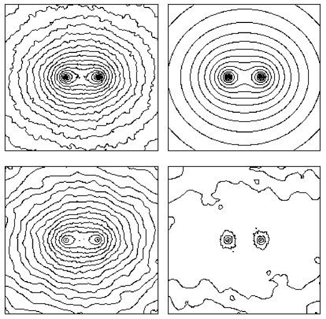
Figure 11 shows the amplitude of $q_{ggm}$ along the $y=0$ axis, now for galaxies separated by $R_{12}=0.25~{}h^{-1}$ Mpc. From this plot one can see that on larger scales $q_{ggm}$ drops off slowly, but on small scales there are holes around the galaxy pairs. On scales larger than the galaxy separation, $q_{ggm}$ is mostly radially symmetric about the center. In Figure 12 we show the radial profile of $q_{ggm}$ about the center of two galaxies with $R_{12}=0.05h^{-1}$ Mpc. On scales comparable to $R_{12}$, $q_{ggm}$ is rising as it climbs out of the hole and at larger scales it drops off.

Figure 11: A slice through the 2D $q_{ggm}(x,y)$ along the $y=0$ axis which is the direction passing through the two galaxy centers. The galaxy separation is $R_{12}=0.25~{}h^{-1}$ Mpc. At small scales one can clearly see the holes around the galaxies (which may be an unrealistic feature of halo models). On larger scales $q_{ggm}$ drops off slowly.

Figure 12: The radial profile of the 2D $q_{ggm}$ for closer galaxy pairs, $R_{12}=50~{}h^{-1}$ kpc. The inner part of the curve is still rising as $q_{ggm}$ climbs out of the holes. At scales of a few times $R_{12}$ the profile is fairly radially symmetric and decreases slowly. There is an apparent bump at $1.5~{}h^{-1}$ Mpc where the two-halo term typically begins to dominate.

9 Extracting Information from Shear Measurements

As we saw in Section 4, we can use the method of galaxy-galaxy lensing (GGL) to measure the galaxy-mass correlation function. By measuring the tangential shear around lens galaxies, one can reconstruct $w_{gm}(R)$ and then invert the projection to obtain $\xi_{gm}(r)$. In Section 5, we calculated the 2D mass density around projected pairs of galaxies and showed how it was related to the GGM3PCF. We will now discuss how to measure this statistic from shear data using the SDSS as our fiducial data set. We assume we have a spectroscopic sample of galaxies with measured redshifts that we will use as our lens galaxies and a fainter photometric sample of galaxies without redshifts (though possibly with photometric redshifts) that we will use as source galaxies.

Our first task is to find pairs of lens galaxies out to some maximum projected radius. We will also want to impose a cut on their redshift difference. As we discussed in Section 5, this cut imposes an effective cut in the radial direction $L_{U}$. One will probably want to keep this fairly large, such as $30-50~{}h^{-1}$ Mpc, to limit the effects of redshift distortions on the interpretation of the results.

Once we have a galaxy pair, we rotate the local coordinate frame to align them along the x-axis. There was no need to do this with GGL since the average tangential shear around single galaxies must be isotropic. In that case, we just chose a set of radial bins and averaged the tangential shear for objects in each bin. Now we have a pair of galaxies which breaks this spherical symmetry and therefore need to deal with both components of the shear and keep track of both $x,y$ components of the source galaxies. Thus, we now have a 2D problem and will measure a 2D shear map rather than just a 1D shear profile. We choose an $x,y$ grid on which to store the ellipticity measurements and use the rotated $x,y$ coordinates of the source galaxies to calculate which pixel each source galaxy belongs to (for a given lens galaxy pair).

We want to build up a map of the average source galaxy ellipticity stacked (averaged) over many lens galaxy pairs. However, since the lens galaxy pairs have a range of projected separations, we also need to bin in this separation, $R_{12}$, as well and therefore produce a shear map for each $R_{12}$ bin. If we bin too coarsely, this will have the effect of blurring together different $R_{12}$ correlation functions and we lose information. If we bin too finely, the number of lens pairs per bin becomes smaller and the shot noise will overwhelm the signal. With real data, one would also want to bin the len galaxy sample by luminosity and perhaps by color, but we no not have that information in our simulation.

The fact that this is a 2D problem with no exact symmetries means that instead of just a few radial bins one might have hundreds of pixels. In addition, as noted above, one has to separate the lens galaxy pairs into several bins of $R_{12}$. Because of this, one cannot expect a high signal-to-noise ratio in any particular shear map pixel since the signal-to-noise ratio is only of order 1-10 in present measurements of the GGL signal from the GM2PCF with only a few radial bins. However, as we will see, one can use approximate symmetries to make measurements with signal-to-noise similar to the simpler GGL measurements of the GM2PCF.

To calculate the shear map from $\Sigma(x,y)$ we solve for the 2D lensing potential $\phi(x,y)$ by solving Poisson’s equation (see Section LABEL:section:weak-lensing-basics). Then we numerically differentiate $\phi$ to obtain the shear components $\gamma_{1}$ and $\gamma_{2}$. We will use as our model the density $\Sigma(x,y)$ for $R_{12}=0.8~{}h^{-1}$ Mpc. For simplicity, in calculating $\Sigma_{crit}$, we choose all the lens redshifts to be $z_{L}=0.1$ and all the source redshifts to be $z_{S}=0.3$, similar to the mean lens and source redshifts used in the SDSS lensing measurements. We display the shear map for a box of width $6~{}h^{-1}$ Mpc calculated from this density in Figure 13. In Figure 14 we show a higher resolution image of the region close to the galaxy pair. This smaller region is $1.2~{}h^{-1}$ Mpc on a side. From the first plot one can see that at larger radius the shear is mostly tangential though one can notice a residual ellipticity to the pattern that drops off as one goes out further.

Figure 13: The mean shear map around pairs of galaxies of separation $R_{12}=0.8~{}h^{-1}$ Mpc. The size of the region is $6~{}h^{-1}$ Mpc on a side. At larger scales the signal is mostly tangential but in the middle the signal is more complicated. See next figure for a more detailed view.

Figure 14: A zoom of the previous figure of the central region near the two galaxies. The scale is $1.2~{}h^{-1}$ Mpc on a side. In the middle, the mostly-tangential shear from each galaxy adds constructively. There is also a ring of destructive interference where the shear from each galaxy is in the opposite direction of the other.

In the central region, the shear map is more complicated and it helps to look at the second plot, Figure 14. To understand this pattern one has to remember that the shear is a vector (technically a spin-2 field) and this pattern is the superposition of two terms which are mostly tangential about the two galaxies. Because it is a vector, there can be constructive and destructive interference. The region in the middle is a region of constructive interference where the shear from each galaxy has the same phase (i.e., direction), so this is where the shear is the largest. There is also a ring of destructive interference where the shear from each galaxy cancels out the other and no net shear is produced.

In Figure 15 we show the individual shear components around the same 2D density map. Here the scale is $4.2~{}h^{-1}$ Mpc on a side. The top left shows $\kappa=\Sigma/\Sigma_{crit}$. Top right shows the magnitude of the shear $|\gamma|=\sqrt{\gamma_{1}^{2}+\gamma_{2}^{2}}$. The bottom panels show $\gamma_{1}$ and $\gamma_{2}$ from left to right respectively.

Figure 15: Displayed are $\log\kappa$ (top left); $|\gamma|$ (top right); $\gamma_{1}$ (bottom left); $\gamma_{2}$ (bottom right) The galaxy separation is $R_{12}=0.8~{}h^{-1}$ Mpc and the box size is $4.2~{}h^{-1}$ Mpc on a side.

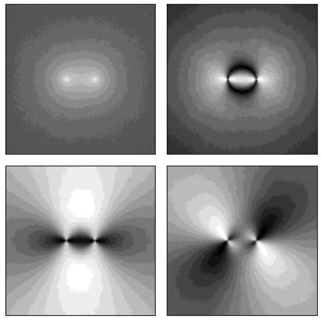
The $\kappa$ plot shows the bimodal pattern on small scales and elliptical contours on larger scales. The plot of $|\gamma|$ shows a dark ring where the net shear is zero due to the interference and the bright spots where the shear is largest in the center and just on the outsides of where the galaxies are. It also shows how $|\gamma|$ has elliptical contours on larger scales.

In Figure 16 we show the tangential shear $\gamma_{T}$ and the radial shear $\gamma_{R}$ defined as $\gamma_{T}\equiv-\gamma_{1}\cos 2\theta-\gamma_{2}\sin 2\theta$ and $\gamma_{R}\equiv-\gamma_{2}\cos 2\theta+\gamma_{1}\sin 2\theta$ where $\theta$ is the angle from the midpoint of the $x$-axis. The top left is $\gamma_{T}$ and top right $\gamma_{R}$. The bottom left is $|\gamma_{T}|/|\gamma|$ and bottom right is $|\gamma_{T}|/|\gamma|$. In the bottom color scale, black is zero and white is 1. The bottom plots show how at large scales the shear is almost entirely tangential whereas at small scales the pattern is complicated and both $\gamma_{T}$ and $\gamma_{R}$ make contributions.

Figure 16: Displayed are $\gamma_{T}$ (top left); $\gamma_{R}$ (top right); $|\gamma_{T}|/|\gamma|$ (bottom left); $|\gamma_{R}|/|\gamma|$ (bottom right); The galaxy separation is $R_{12}=0.8~{}h^{-1}$ Mpc and the box size is $4.2~{}h^{-1}$ Mpc on a side.

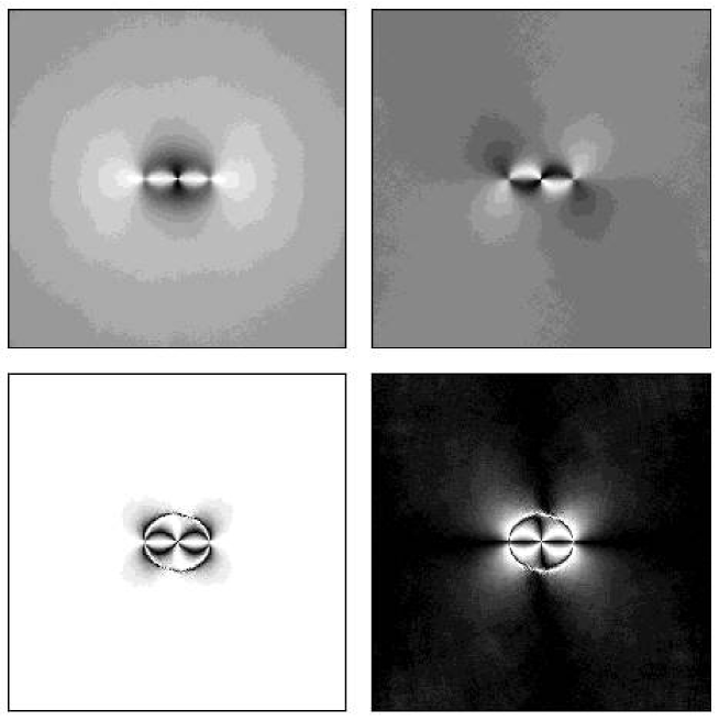
This is an example of how there is an approximate symmetry that allows one to ignore the radial shear component at large scales. On these scales one can just measure the tangential component and see how its magnitude changes as a function of $R$ and $\theta$. For example Figure 17 shows the tangential shear in an annulus (centered between the galaxies) of radius $R=2.0\pm 0.1~{}h^{-1}$ Mpc, as a function of $\theta$ (measured from the $x$-axis), divided by the mean value in the annulus. A quadrupole pattern is evident and we over-plot the function $\gamma_{T}/\gamma_{To}(\theta)=(1+\epsilon\cos 2\theta)$ with $\epsilon=0.07$. One can relate the moments of the shear map to moments of $\kappa$ through methods developed by Schneider & Bartelmann (1997); Natarajan & Refregier (2000).

Figure 17: The tangential shear in an annulus of radius $R=2.0\pm 0.1~{}h^{-1}$ Mpc, centered between lens galaxies divided by the mean value in the annulus as a function of $\theta$. A quadrupole pattern is evident and we over-plot a pure quadrupole $\gamma_{T}/\gamma_{To}(\theta)=(1+\epsilon\cos 2\theta)$ with and ellipticity parameter $\epsilon=0.07$.

10 Estimate of signal-to-noise ratios

So far we have calculated the shear signal we expect around foreground galaxy pairs, and now we investigate the amount of noise we expect. The noise in a weak lensing measurement is almost entirely due to shot noise from galaxy shapes, although on the largest scales, sample variance can increase the variance and add some covariance (Sheldon et al., 2004). We will only discuss the shot noise since it is the dominant source of noise on scales less than a few Mpc. The shot noise on a particular measurement of $\gamma_{i}$ is about $0.2/\sqrt{N}$, where $0.2$ represents the RMS intrinsic ellipticity of galaxies divided by 2. The number $N$ for GGL is the number of lens-source galaxy pairs in a given radial bin. For our analysis, we have pairs of lens galaxies and so $N$ is the number of lens-lens-source triplets in a given measurement bin. We now estimate what this number $N$ will be.

If we have $N_{p}$ foreground galaxy pairs in a given projected separation bin, $R_{12}$, and a 2D number density $\sigma_{S}$ of source galaxies, then the number of triplets is just $N=N_{p}\sigma_{S}dA$ where $dA$ is some surface area element in which we estimate the shear. We have assumed that the source density $\sigma_{S}$ is uncorrelated with the density of foreground pairs, which should be correct if lens and source galaxies are at different redshifts. To estimate the number of lens galaxy pairs, we calculate the average number of neighbors per galaxy, $\langle n_{p}\rangle$, in a thin annulus about projected separation $R$ of width $\Delta R$. This is just an integral over the galaxy-galaxy correlation function (Peebles, 1980),

$$\langle n_{p}\rangle = n_{g}~{}2\pi~{}R~{}\Delta R~{}\int_{-L_{U}/2}^{L_{U}/2}du~{}(1+\xi_{gg}(\sqrt{u^{2}+R^{2}}))$$ (41)

$$= n_{g}~{}2\pi~{}R~{}\Delta R~{}(L_{U}+w_{gg}(R))$$ (42)

where $n_{g}$ is the 3D number density of lens galaxies. The total number of pairs in this bin is then $N_{p}=N_{L}\langle n_{p}\rangle/2$, where $N_{L}$ is the total number of lens galaxies. The number $N_{L}$ is just the number density $n_{g}$ times the comoving volume probed by the survey, $V$. Finally we can write the number of lens-lens-source triplets, $N$, in surface area element $dA$ for lens pairs separated by $R\pm\Delta R/2$ as

$$N=\pi~{}n_{g}^{2}~{}V~{}R~{}\Delta R~{}(L_{U}+w_{gg}(R))~{}\sigma_{S}~{}dA$$ (43)

The galaxy number density in our simulation is $n_{g}=4.56\times 10^{-3}h^{3}\mbox{Mpc}^{-3}$, which roughly corresponds to an effective absolute magnitude cut of $M_{r}<-20$. For this absolute magnitude cut, the SDSS probes an effective survey volume of approximately $V=1.2~{}f_{sky}~{}\times 10^{8}h^{-3}\mbox{Mpc}^{3}$ (Tegmark et al., 2003), where $f_{sky}$ is the fraction of the sky covered. For the SDSS, $f_{sky}$ will eventually be close to 1/4. The number density of source galaxies used for lensing from Sheldon et al. (2004) is $3200/deg^{2}$. The area element dA in $deg^{2}$ is dA=$(180~{}dx/\pi D(z_{L}))^{2}$ where $dx$ is the pixel size in physical units that we will use for our shear map and $D(z_{L})$ is the angular diameter distance to redshift $z_{L}$. We will choose $z_{L}=0.1$, the median redshift for the SDSS spectroscopic survey, and $7000~{}deg^{2}$ for the estimated sky coverage of the completed SDSS, which gives $f_{sky}=0.17$. With these numbers our expression for $N$ becomes

$$N=2.0\times 10^{5}h^{5}Mpc^{-5}~{}R~{}\Delta R~{}(L_{U}+w_{gg}(R))~{}dx^{2}$$ (44)

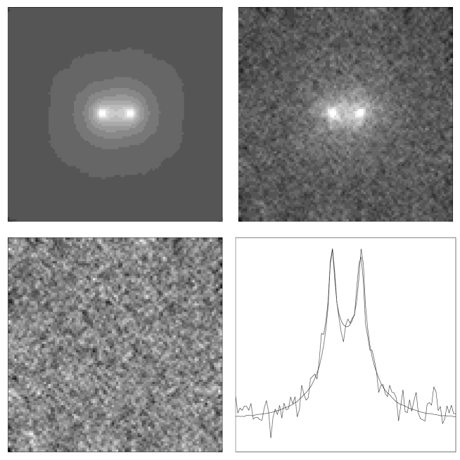
With this formula we are able to add noise to our shear maps that should correspond to what we will see if we do an analysis similar to Sheldon et al. (2004) with SDSS data in the near future to measure the mass density around pairs. We take our predicted shear map shown in Figure 13, which corresponds to $R_{12}=0.8~{}h^{-1}$ Mpc, and add Gaussian noise with $\sigma=0.2/\sqrt{N}$ to each component of the shear. The resulting noisy shear map is shown in Figure 18. The basic tangential pattern can still be seen behind the noise.

Figure 18: The same shear map of Figure 13 when Gaussian noise, expected from the SDSS, is added.

We can now process both the noisy shear map and the noiseless one to reconstruct $\kappa$ with a KS mass reconstruction algorithm. We use the “direct method” of Lombardi & Bertin (1999). This inversion routine reconstructs the mass map by solving for the Fourier modes on a chosen grid that minimize the functional

$$S=\frac{1}{2}\int_{A}d^{2}x||\nabla\kappa(\vec{x})-\vec{u}(\vec{x})||$$ (45)

where

$$\vec{u}(\vec{x})\equiv\left(\begin{array}[]{c}\gamma_{1,1}+\gamma_{2,1}\\ \gamma_{2,1}-\gamma_{1,2}\end{array}\right)$$ (46)

The Euler-Lagrange equations of this functional are just Equations 8 that we saw related the measured shear to $\kappa$. This routine is linear and can be done quickly with Fast Fourier Transforms. Unlike the earliest KS algorithms this one does not have edge effect biases other than slightly increased noise in the bounding bins. The process involves choosing a grid scale, averaging the shear in the grid bins, calculating $\vec{u}(\vec{x})$ by finite differencing the shear values, and then running Lombardi and Bertin’s routine (which is publicly available) on the array $\vec{u}$. The resulting reconstruction will be degraded in resolution for two reasons. First, one will usually want to choose a grid scale that gives reasonable signal-to-noise per pixel. This is purely a pixelization effect and structures smaller than the pixel scale will be lost. Second, the reconstruction algorithm which differences neighbors introduces an effective smoothing between neighboring pixels.

We display the reconstruction in Figure 19. The top right is the original $\kappa$ binned down to the same grid resolution of the reconstruction. The top right shows the $\kappa$ recovered from the noisy shear map via the reconstruction algorithm. The bottom left shows the residual, which is consistent with zero. The bottom right shows a slice through both maps that intersects both peaks around the galaxies. Since the reconstruction cannot recover the constant mass sheet we have subtracted off the mean from each map before plotting.

Figure 19: The top left shows the original $\kappa$ map binned down to the same resolution of the reconstructed one. The top right shows the reconstruction obtained by inverting the noisy shear map. The bottom left is the residual from subtracting the top two maps. One can see that the residual is consistent with zero but the noise is also correlated over the scale of just a couple of pixels. The bottom right plot shows a slice through the two peaks for both densities. One can see that the reconstruction works very well. The means have been subtracted off both maps before plotting since this constant mass sheet is unmeasurable.

11 Conclusion

We have calculated the weak lensing shear around pairs of galaxies and related it directly to the 3D galaxy-galaxy-mass three-point correlation function. We have shown that the 2D mass profile can be reconstructed from the shear map around galaxy pairs and we have discussed how to interpret this in terms of the correlation functions. With our N-body simulation and HOD bias model we have calculated the expected signal and have estimated the amount of noise to be expected in a model survey similar to the Sloan Digital Sky Survey. Although this prediction is only meant to be a first attempt at estimating the effect and does not exhaust the possibilities we predict that this signal may be measurable with current SDSS lensing data. The anisotropic dark matter profile about two galaxies extends far away from their center and will produce an anisotropic tangential shear profile. Measurements confirming this will be difficult to reconcile with alternative theories of gravity that need to produce weak lensing shear without any extended anisotropic dark matter halos. On the other hand we have seen that they are a natural prediction of CDM. The three-point function better specifies how mass traces galaxies and so provides more detailed information over that contained in the isotropic galaxy-mass two-point correlation function. This exact form of the measured galaxy-galaxy-mass correlation function will provide additional constraints on galaxy bias models that govern how galaxies trace the underlying dark matter.

12 Acknowledgments

I would like to thank Joshua Frieman, Erin Sheldon and Andreas Berlind for useful discussions. I would also like to thank Martin White for providing the N-body simulations and Andreas for providing the galaxy occupation. I would also like to thank the Aspen Center for Physics where some of this work was completed.

References

- Bartelmann & Schneider (2001) Bartelmann, M. & Schneider, P. 2001
- Benson et al. (2000) Benson, A. J., Cole, S., Frenk, C. S., Baugh, C. M., & Lacey, C. G. 2000, MNRAS, 311, 793
- Berlind & Weinberg (2002) Berlind, A. A. & Weinberg, D. H. 2002, ApJ, 575, 587
- Berlind et al. (2003) Berlind, A. A., Weinberg, D. H., Benson, A. J., Baugh, C. M., Cole, S., Davé, R., Frenk, C. S., Jenkins, A., Katz, N., & Lacey, C. G. 2003, ApJ, 593, 1
- Bernardeau et al. (2002) Bernardeau, F., Colombi, S., Gaztanaga, E., & Scoccimarro, R. 2002, Phys. Rep., 367, 1
- Binney & Tremaine (1987) Binney, J. & Tremaine, S. 1987
- Blanton et al. (2003) Blanton, M. R., Hogg, D. W., Bahcall, N. A., Brinkmann, J., Britton, M., Connolly, A. J., Csabai, I., Fukugita, M., Loveday, J., Meiksin, A., Munn, J. A., Nichol, R. C., Okamura, S., Quinn, T., Schneider, D. P., Shimasaku, K., Strauss, M. A., Tegmark, M., Vogeley, M. S., & Weinberg, D. H. 2003, ApJ, 592, 819
- Brainerd et al. (1996) Brainerd, T. G., Blandford, R. D., & Smail, I. 1996, ApJ, 466, 623
- Burles et al. (2001) Burles, S., Nollett, K. M., & Turner, M. S. 2001, Phys.Rev.D, 63, 63512
- Clowe et al. (1998) Clowe, D., Luppino, G. A., Kaiser, N., Henry, J. P., & Gioia, I. M. 1998, ApJ, 497, L61+
- Davis et al. (1985) Davis, M., Efstathiou, G., Frenk, C. S., & White, S. D. M. 1985, ApJ, 292, 371
- dell’Antonio & Tyson (1996) dell’Antonio, I. P. & Tyson, J. A. 1996, ApJ, 473, L17+
- Eisenstein & Hu (1998) Eisenstein, D. J. & Hu, W. 1998, ApJ, 496, 605
- Evrard et al. (2002) Evrard, A. E., MacFarland, T. J., Couchman, H. M. P., Colberg, J. M., Yoshida, N., White, S. D. M., Jenkins, A., Frenk, C. S., Pearce, F. R., Peacock, J. A., & Thomas, P. A. 2002, ApJ, 573, 7
- Fahlman et al. (1994) Fahlman, G., Kaiser, N., Squires, G., & Woods, D. 1994, ApJ, 437, 56
- Feldman et al. (2001) Feldman, H. A., Frieman, J. A., Fry, J. N., & Scoccimarro, R. 2001, Physical Review Letters, 86, 1434
- Fischer et al. (2000) Fischer, P., McKay, T. A., Sheldon, E., Connolly, A., Stebbins, A., Frieman, J. A., Jain, B., Joffre, M., Johnston, D., Bernstein, G., Annis, J., Bahcall, N. A., Brinkmann, J., Carr, M. A., Csabai, I., Gunn, J. E., Hennessy, G. S., Hindsley, R. B., Hull, C., Ivezić, Ž., Knapp, G. R., Limmongkol, S., Lupton, R. H., Munn, J. A., Nash, T., Newberg, H. J., Owen, R., Pier, J. R., Rockosi, C. M., Schneider, D. P., Smith, J. A., Stoughton, C., Szalay, A. S., Szokoly, G. P., Thakar, A. R., Vogeley, M. S., Waddell, P., Weinberg, D. H., York, D. G., & The SDSS Collaboration. 2000, AJ, 120, 1198
- Freedman et al. (2001) Freedman, W. L., Madore, B. F., Gibson, B. K., Ferrarese, L., Kelson, D. D., Sakai, S., Mould, J. R., Kennicutt, R. C., Ford, H. C., Graham, J. A., Huchra, J. P., Hughes, S. M. G., Illingworth, G. D., Macri, L. M., & Stetson, P. B. 2001, ApJ, 553, 47
- Frieman & Gaztañaga (1999) Frieman, J. A. & Gaztañaga, E. 1999, ApJ, 521, L83
- Fry (1984) Fry, J. N. 1984, ApJ, 279, 499
- Fry & Seldner (1982) Fry, J. N. & Seldner, M. 1982, ApJ, 259, 474
- Gott & Turner (1979) Gott, J. R. & Turner, E. L. 1979, ApJ, 232, L79
- Griffiths et al. (1996) Griffiths, R. E., Casertano, S., Im, M., & Ratnatunga, K. U. 1996, MNRAS, 282, 1159
- Groth & Peebles (1977) Groth, E. J. & Peebles, P. J. E. 1977, ApJ, 217, 385
- Hammer (1991) Hammer, F. 1991, ApJ, 383, 66
- Hoekstra et al. (2003) Hoekstra, H., Franx, M., Kuijken, K., Carlberg, R. G., & Yee, H. K. C. 2003, MNRAS, 340, 609
- Huchra et al. (1999) Huchra, J. P., Vogeley, M. S., & Geller, M. J. 1999, VizieR Online Data Catalog, 212, 10287
- Hudson et al. (1998) Hudson, M. J., Gwyn, S. D. J., Dahle, H., & Kaiser, N. 1998, ApJ, 503, 531
- Irgens et al. (2002) Irgens, R. J., Lilje, P. B., Dahle, H., & Maddox, S. J. 2002, ApJ, 579, 227
- Jenkins et al. (1998) Jenkins, A., Frenk, C. S., Pearce, F. R., Thomas, P. A., Colberg, J. M., White, S. D. M., Couchman, H. M. P., Peacock, J. A., Efstathiou, G., & Nelson, A. H. 1998, ApJ, 499, 20
- Jenkins et al. (2001) Jenkins, A., Frenk, C. S., White, S. D. M., Colberg, J. M., Cole, S., Evrard, A. E., Couchman, H. M. P., & Yoshida, N. 2001, MNRAS, 321, 372
- Jimenez et al. (1996) Jimenez, R., Thejll, P., Jorgensen, U. G., MacDonald, J., & Pagel, B. 1996, MNRAS, 282, 926
- Joffre et al. (2000) Joffre, M., Fischer, P., Frieman, J., McKay, T., Mohr, J. J., Nichol, R. C., Johnston, D., Sheldon, E., & Bernstein, G. 2000, ApJ, 534, L131
- Johnston et al. (2004) Johnston, D., Sheldon, E., & Frieman, J. 2004, In preparation
- Kaiser & Squires (1993) Kaiser, N. & Squires, G. 1993, ApJ, 404, 441
- Kauffmann et al. (1999) Kauffmann, G., Colberg, J. M., Diaferio, A., & White, S. D. M. 1999, MNRAS, 303, 188
- Kauffmann & White (1993) Kauffmann, G. & White, S. D. M. 1993, MNRAS, 261, 921
- Kneib et al. (1996) Kneib, J.-P., Ellis, R. S., Smail, I., Couch, W. J., & Sharples, R. M. 1996, ApJ, 471, 643
- Lacey & Cole (1993) Lacey, C. & Cole, S. 1993, MNRAS, 262, 627
- Lombardi & Bertin (1999) Lombardi, M. & Bertin, G. 1999, A&A, 348, 38
- Luppino & Kaiser (1997) Luppino, G. A. & Kaiser, N. 1997, ApJ, 475, 20
- Ma & Fry (2000a) Ma, C. & Fry, J. N. 2000a, ApJ, 543, 503
- Ma & Fry (2000b) —. 2000b, ApJ, 531, L87
- McClelland & Silk (1977) McClelland, J. & Silk, J. 1977, ApJ, 217, 331
- McKay et al. (2001) McKay, T. A. et al. 2001
- Milgrom (1983) Milgrom, M. 1983, ApJ, 270, 365
- Natarajan & Refregier (2000) Natarajan, P. & Refregier, A. 2000, ApJ, 538, L113
- Navarro et al. (1997) Navarro, J. F., Frenk, C. S., & White, S. D. M. 1997, ApJ, 490, 493
- Neyman & Scott (1952) Neyman, J. & Scott, E. L. 1952, ApJ, 116, 144
- Peacock et al. (2001) Peacock, J. A., Cole, S., Norberg, P., Baugh, C. M., Bland-Hawthorn, J., Bridges, T., Cannon, R. D., Colless, M., Collins, C., Couch, W., Dalton, G., Deeley, K., De Propris, R., Driver, S. P., Efstathiou, G., Ellis, R. S., Frenk, C. S., Glazebrook, K., Jackson, C., Lahav, O., Lewis, I., Lumsden, S., Maddox, S., Percival, W. J., Peterson, B. A., Price, I., Sutherland, W., & Taylor, K. 2001, Nature, 410, 169
- Peacock & Smith (2000) Peacock, J. A. & Smith, R. E. 2000, MNRAS, 318, 1144
- Peebles (1980) Peebles, P. 1980, The Large Scale Structure of the Universe (Princeton University Press)
- Peebles (1974a) Peebles, P. J. E. 1974a, A&A, 32, 197
- Peebles (1974b) —. 1974b, A&A, 32, 197
- Peebles & Groth (1975) Peebles, P. J. E. & Groth, E. J. 1975, ApJ, 196, 1
- Pen (1998) Pen, U. 1998, ApJ, 504, 601
- Perlmutter et al. (1999) Perlmutter, S., Aldering, G., Goldhaber, G., Knop, R. A., Nugent, P., Castro, P. G., Deustua, S., Fabbro, S., Goobar, A., Groom, D. E., Hook, I. M., Kim, A. G., Kim, M. Y., Lee, J. C., Nunes, N. J., Pain, R., Pennypacker, C. R., Quimby, R., Lidman, C., Ellis, R. S., Irwin, M., McMahon, R. G., Ruiz-Lapuente, P., Walton, N., Schaefer, B., Boyle, B. J., Filippenko, A. V., Matheson, T., Fruchter, A. S., Panagia, N., Newberg, H. J. M., Couch, W. J., & The Supernova Cosmology Project. 1999, ApJ, 517, 565
- Press & Schechter (1974) Press, W. H. & Schechter, P. 1974, ApJ, 187, 425
- Riess et al. (1998) Riess, A. G., Filippenko, A. V., Challis, P., Clocchiatti, A., Diercks, A., Garnavich, P. M., Gilliland, R. L., Hogan, C. J., Jha, S., Kirshner, R. P., Leibundgut, B., Phillips, M. M., Reiss, D., Schmidt, B. P., Schommer, R. A., Smith, R. C., Spyromilio, J., Stubbs, C., Suntzeff, N. B., & Tonry, J. 1998, AJ, 116, 1009
- Saunders et al. (1992) Saunders, W., Rowan-Robinson, M., & Lawrence, A. 1992, MNRAS, 258, 134
- Schneider & Bartelmann (1997) Schneider, P. & Bartelmann, M. 1997, MNRAS, 286, 696
- Scoccimarro et al. (2001a) Scoccimarro, R., Feldman, H. A., Fry, J. N., & Frieman, J. A. 2001a, ApJ, 546, 652
- Scoccimarro et al. (2001b) Scoccimarro, R., Sheth, R. K., Hui, L., & Jain, B. 2001b, ApJ, 546, 20
- Scranton (2003) Scranton, R. 2003, MNRAS, 339, 410
- Seitz & Schneider (2001) Seitz, S. & Schneider, P. 2001, A&A, 374, 740
- Seljak (2000) Seljak, U. 2000, MNRAS, 318, 203
- Sheldon et al. (2004) Sheldon, E., Johnston, D., Frieman, J., Scranton, R., McKay, T., Connolly, A., & SDSS collaboration. 2004, In preparation
- Sheth & Tormen (1999) Sheth, R. K. & Tormen, G. 1999, MNRAS, 308, 119
- Smith et al. (2001) Smith, D. R., Bernstein, G. M., Fischer, P., & Jarvis, M. 2001, ApJ, 551, 643
- Spergel et al. (2003) Spergel, D. N., Verde, L., Peiris, H. V., Komatsu, E., Nolta, M. R., Bennett, C. L., Halpern, M., Hinshaw, G., Jarosik, N., Kogut, A., Limon, M., Meyer, S. S., Page, L., Tucker, G. S., Weiland, J. L., Wollack, E., & Wright, E. L. 2003, ApJS, 148, 175
- Takada & Jain (2003a) Takada, M. & Jain, B. 2003a, MNRAS, 340, 580
- Takada & Jain (2003b) —. 2003b, MNRAS, 344, 857
- Tegmark et al. (2003) Tegmark, M. et al. 2003
- Totsuji & Kihara (1969) Totsuji, H. & Kihara, T. 1969, PASJ, 21, 221
- Tyson & Fischer (1995) Tyson, J. A. & Fischer, P. 1995, ApJ, 446, L55+
- Tyson et al. (1984) Tyson, J. A., Valdes, F., Jarvis, J. F., & Mills, A. P. 1984, ApJ, 281, L59
- White (2002) White, M. 2002, ApJS, 143, 241
- White (2003) White, M. J. 2003
- White & Frenk (1991) White, S. D. M. & Frenk, C. S. 1991, ApJ, 379, 52
- White & Rees (1978) White, S. D. M. & Rees, M. J. 1978, MNRAS, 183, 341
- Wilson et al. (2001) Wilson, G., Kaiser, N., Luppino, G. A., & Cowie, L. L. 2001, ApJ, 555, 572
- York & SDSS collaboration (2000) York, D. G. & SDSS collaboration. 2000, AJ, 120, 1579
- Zehavi et al. (2003) Zehavi, I. et al. 2003, ApJ, 608 ,16