Quasar Spectrum Classification with PCA - II:
Introduction of Five Classes, Artificial Quasar Spectrum, the Mean Flux Correction Factor $\delta F$, and the Identification of Emission Lines in the Ly$\alpha$ Forest

Abstract

We investigate the variety in quasar UV spectra ($\lambda\lambda$1020-1600) with emphasis on the weak emission lines in the Ly$\alpha$ forest region using principal component analysis (PCA). This paper is a continuation of Suzuki et al. (2005, Paper I), but with a different approach. We use 50 smooth continuum fitted quasar spectra (0.14 $<z<$ 1.04) taken by the Hubble Space Telescope (HST) Faint Object Spectrograph. There are no broad absorption line quasars included in these 50 spectra. The first, second and third principal component spectra (PCS) account for 63.4, 14.5 and 6.2% of the variance respectively, and the first seven PCS take 96.1% of the total variance. The first PCS carries Ly$\alpha$, Ly$\beta$ and high ionization emission line features (O VI, N V, Si IV, C IV) that are sharp and strong. The second PCS has low ionization emission line features (Fe II, Fe III, Si II, C II) that are broad and rounded. Three weak emission lines in the Ly$\alpha$ forest are identified as Fe II $\lambda 1070.95$, Fe II+Fe III $\lambda 1123.17$, and C III^∗ $\lambda 1175.88$. Using the first two standardized PCS coefficients, we introduce five classifications: Class Zero and Classes I-IV. These classifications will guide us in finding the continuum level in the Ly$\alpha$ forest. We show that the emission lines in the Ly$\alpha$ forest become prominent for Classes III and IV. By actively using PCS, we can generate artificial quasar spectra that are useful in testing the detection of quasars, DLAs, and the continuum calibration. We provide 10,000 artificially generated spectra. We show that the power-law extrapolated continuum is inadequate to perform precise measurements of the mean flux in the Ly$\alpha$ forest because of the weak emission lines and the extended tails of Ly$\alpha$ and Ly$\beta$/O VI emission lines. We introduce a correction factor $\delta F$ so that the true mean flux $\langle F\rangle$ can be related to $\langle F_{Power-Law}\rangle$ as measured using power-law continuum extrapolation by : $\langle F\rangle=\langle F_{Power-Law}\rangle\cdot\delta F$. The correction factor $\delta F$ ranges from 0.84 to 1.05 with a mean of 0.947 and a standard deviation of 0.031 for our 50 quasars. This result means that using power-law extrapolation we miss 5.3% of flux on average and we show that there are cases where we would miss 16% of flux. These corrections are essential in the study of the intergalactic medium at high redshift in order to achieve precise measurements of physical properties, cosmological parameters, and the reionization epoch.

1 Introduction

It is important for the study of quasar absorption lines to understand the shape of the continua in the Ly$\alpha$ forest from which we study the physical properties of the intergalactic medium (IGM) and extract cosmological parameters (Kirkman et al., 2003; Tytler et al., 2004a). It is the uncertainty of continuum fitting to the Ly$\alpha$ forest that makes precise measurements difficult(Croft et al., 2002a; Suzuki et al., 2003; Jena et al., 2004). Thus, we wish to have a simple and objective quasar spectrum classification scheme that enables us to describe the global shape of the continuum as well as the individual emission line profiles. The principal component analysis (PCA), also known as Karhunen-Loève expansion, is one of the best methods to carry out such classification.

PCA enables one to summarize the information contained in a large data set, and it is widely used in many areas of astronomy (Cabanac et al., 2002, and references therein). Francis et al. (1992) applied PCA to quasar spectra using 232 quasar spectra (1.8 $<$ z $<$ 2.2 ; $\lambda\lambda 1150-2000$) from the Large Bright Quasar Survey (LBQS; Hewett et al., 1995, 2001). They showed that the first three principal components account for 75% of the variance. Boroson & Green (1992) used 87 low redshift quasar spectra ( z $<$ 0.5) and showed the anticorrelation between the equivalent width of Fe II and [O III] and the correlation between the luminosity, the strength of He II $\lambda$4686, and the slope index $\alpha_{ox}$. Boroson (2002) investigated the relation between the first two principal components and the physical properties such as black hole mass, luminosity, and radio activity. Shang et al. (2003) studied 22 low redshift UV and optical quasar spectra (z $<$ 0.5 ; $\lambda\lambda 1171-6607$) and showed the relation between the first principal component and the Baldwin effect, which is the anticorrelation between the luminosity and the equivalent width of the C IV emission line. Yip et al. (2004) applied PCA to the 16,707 Sloan Digital Sky Survey quasar spectra (0.08 $<z<$ 5.41 ; $\lambda\lambda 900-8000$) and reported that the spectral classification depends on the redshift and luminosity, and that there is no compact set of eigenspectra that can describe the majority of variations. They also showed the relationship between eigencoefficients and the Baldwin effect.

In Suzuki et al. (2005, hereafter Paper I) we analyzed 50 continua fitted quasar spectra taken by the Hubble Space Telescope (HST) Faint Object Spectrograph. Since they are at low redshifts ($0.14<z<1.04$), and the Ly$\alpha$ forest lines are not so dense, we can see and correctly fit the continuum to the spectra. Using PCA we attempted to predict the continuum in the Ly$\alpha$ forest where the continuum levels are hard to see because of the abundance of the IGM absorptions. Although we succeeded in predicting the shape of the weak emission lines in the Ly$\alpha$ forest region, our prediction suffers systematic errors of $3-30$%. This paper is a continuation of Paper I, but with a different approach.

The goal of this paper is to explore the variety of quasar UV spectra in the following manner: 1. we clarify the PCA formulation in order to describe quasar UV spectra quantitatively (§3) using eigenspectra or the principal component spectra (PCS), 2. we introduce five classes of quasar UV spectra to help us understand the variety of quasar spectra qualitatively (§5), 3. we introduce the idea of artificial quasar spectra (§4) and 4. the mean flux correction factor $\delta F$ (§6), and 5. we report the identities of three weak emission lines in the Ly$\alpha$ forest (Appendix).

2 Data

We use the same 50 HST FOS spectra from Paper I, and the detailed description is therein. Here we summarize the 50 HST spectra. These 50 quasar spectra are a subset of the 334 high resolution HST FOS spectra (R $\sim$ 1300) collected and calibrated by Bechtold et al. (2002) which include all of the HST QSO Absorption Line Key Project’s data (Bahcall et al., 1993, 1996; Jannuzi et al., 1996). Bechtold et al. (2002) identified both intergalactic and interstellar medium lines and corrected for Galactic extinction.

For each spectrum, we combined the individual exposures and remeasured the redshift using the peak of the Ly$\alpha$ emission line. Then we brought the spectrum to the rest frame and rebinned it into 0.5 Å pixels. We masked the identified absorption lines and fitted a smooth Chebyshev polynomial curve. We normalized the flux by taking the average of 21 pixels around 1280 Å where no emission line is seen.

We chose the wavelength range from 1020 to 1600 Å so that we can cover the Ly$\alpha$ forest between the Ly$\beta$ and the Ly$\alpha$ emission lines while maximizing the number of spectra. We removed broad absorption line (BAL) quasars from the sample since we are interested in emission line profiles and the continuum shape. Lastly, we removed quasars with S/N $<$ 10 per pixel because we cannot extract weak emission line features in low S/N spectra. The redshift range of the 50 spectra is from 0.14 to 1.04 with a mean of 0.58. The average S/N is 19.5 per 0.5 Å binned pixel.

3 PCA & Principal Component Spectrum

3.1 The PCA Formulation

We express a quasar spectrum in Dirac’s “bra ket” form, $|q_{i}\rangle$, which is commonly used in Quantum Mechanics and simplifies our description. We claim that any quasar spectrum, $|q_{i}\rangle$ , is well represented by a reconstructed spectrum, $|r_{im}\rangle$, which is a sum of the mean and the weighted $m$ principal component spectra:

$$|q_{i}\rangle\sim|r_{i,m}\rangle=|\mu\rangle+\sum_{j=1}^{m}c_{ij}|\xi_{j}\rangle$$ (1)

where $i$ refers to a quasar, $|\mu\rangle$ is the mean quasar spectrum, $|\xi_{j}\rangle$ is the $j$th principal component spectrum (PCS), and $c_{ij}$ is its weight. Unlike Quantum Mechanics, the weight, $c_{ij}$, is not a complex number but a real number. We found the covariance and correlation matrix of the 50 quasar spectra in Paper I and by diagonalizing the covariance matrix, we can obtain the PCS. In practice, we found the PCS via a singular value decomposition (SVD) technique from the 50 quasar spectra. The recipes can be found in Francis et al. (1992) and Paper I. Since we designed PCS to be orthonormal:

$$\langle\xi_{i}|\xi_{j}\rangle=\delta_{ij},$$ (2)

where we define the inner product as:

$$\langle x|y\rangle=\int_{1020{\rm\AA}}^{1600{\rm\AA}}x(\lambda)\;y(\lambda)\;d\lambda,$$ (3)

and we can obtain the weights $c_{ij}$ as follows:

$$c_{ij}=\langle q_{i}-\mu|\xi_{j}\rangle.$$ (4)

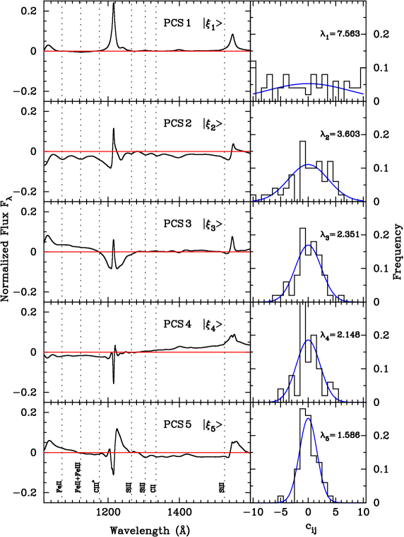
Figure 2: The first five PCS 1-5 are shown in the left panels with the distribution of PCS coefficients $c_{ij}$ on the right. The first PCS takes the Ly$\alpha$, Ly$\beta$ and the high ionization line features (O VI, Si IV, C IV) while the second PCS account for the low ionization lines (Fe II, Fe III, Si II, C II). We expect to have the low ionization lines in the Ly$\alpha$ forest when a quasar has the negative second PCS coefficient. We note that PCS are designed to be orthonormal. The quasar spectra are normalized near 1280 Å and every PCS has zero value near 1280 Å.

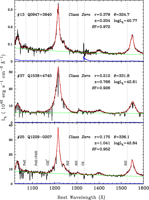
Figure 6: Class Zero ( r $\leq$ 0.668) : The smooth line on the spectrum is the fitted continuum, and the straight solid line is the power-law continuum fit. The line at the bottom is 1-$\sigma$ error of the spectrum. The vertical dotted lines show the wavelengths of emission lines in the Ly$\alpha$ forest and low ionization lines redward of the Ly$\alpha$ emission line. The luminosity, L_λ, is measured at $\lambda$1280 where we normalized the spectra. The emission lines in the Ly$\alpha$ forest are barely seen in the three spectra. A discontinuity of the spectrum is seen in the middle of the spectrum in Q0947+3940 and Q1538+4745. These are due to the different gratings used in the observations to cover the wide range of wavelength. We joined them together by taking the weighted mean, but it does not always give a smooth solution. This discontinuity could be another source of fitting errors.

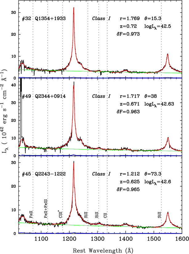
Figure 7: Class I ( r $>$ 0.668, $0\leq\theta<90^{\circ}$): The Ly$\alpha$, Ly$\beta$ and high ionization emission lines are all very sharp and high contrast with the continuum. The low ionization lines, Si II at $\lambda\lambda 1260,1304$, are barely seen. We see no clear sign of emission lines in the Ly$\alpha$ forest, and the power-law continuum is a good approximation. The contrast of Ly$\alpha$ emission peak with the continuum is the highest among the five classes. In Q2344+0914, there is a huge spike at 1030 Å. It is due to an emission line caused by the Earth’s atmosphere. We removed these spikes when we fitted the continuum.

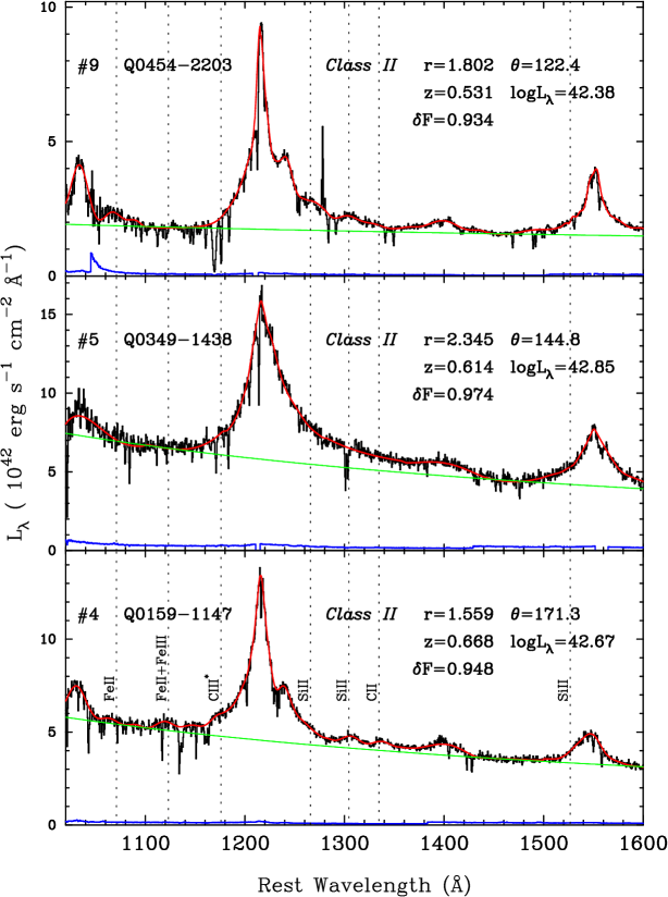
Figure 8: Class II ( $r>0.668$, $90^{\circ}\leq\theta<180^{\circ}$): The Ly$\alpha$ emission peak has a moderate contrast, 4-6, with the continuum, and the emission peak ratio of Ly$\alpha$ and N V is 2-3. The Ly$\alpha$ emission has long tails, and the blueward tail of the fitted continuum does not meet with the power-law continuum until 1120 Å, which is 50 Å below the D_A wavelength definition, 1170 Å. In an extreme case, Q0349-1438 ($r=2.345$), the tail of Ly$\alpha$ emission wings last about 100 Å. Ly$\beta$/O VI, Ly$\alpha$, and C IV emission profiles are triangular, and Si IV $\lambda 1393$ is very broad and rounded. There is no clear separation between Ly$\alpha$ and N V emission lines and no sign of low ionization emission lines.

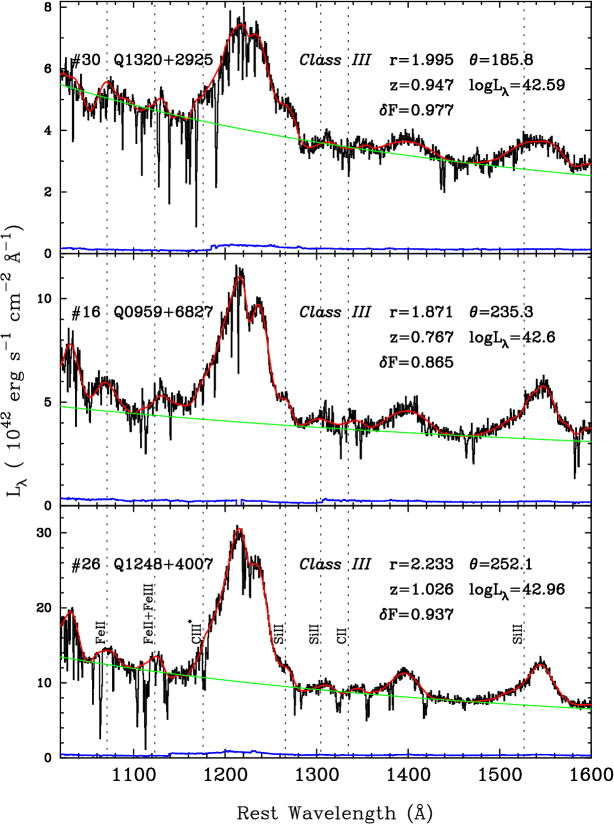
Figure 9: Class III ($r>0.668$, $180^{\circ}\leq\theta<270^{\circ}$ ): The emission line profiles are all broad and rounded. Fe II and Fe III lines are clearly seen in the Ly$\alpha$ forest. The contrast of the Ly$\alpha$ emission line peak with the continuum is the lowest, 2-4, among the five classes. The ratio of Ly$\alpha$ emission peak to N V is also the lowest: 1-2. The C IV profile is asymmetric probably because of the contribution from the Si II $\lambda 1526$ hidden inside the blueward tail of the C IV line.

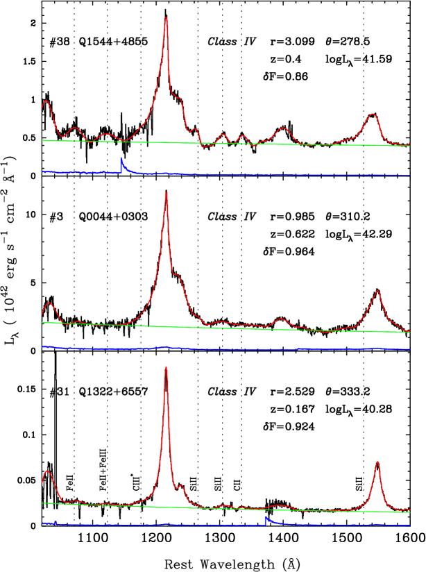
Figure 10: Class IV ($r>0.668$, $270^{\circ}\leq\theta<360^{\circ}$): The high contrast with the continuum and sharp emission profile are the characteristics of this class. Q1544+4855 is an extreme case that has r=3.099. Since it has $\theta=278.5$, it is very close to Class III, but it has the characteristics of Class IV: high Ly$\alpha$ emission line peak contrast and the very sharp line profiles. Unlike a Class III quasar, the peaks of low ionization line profile are very sharp and not rounded. Q1322+6557 has a spike at $\lambda 1040$ that is due to an atmospheric emission line. The fitted spectrum removed the spike for analysis.

We show the mean spectrum in Figure 1 and the first 10 PCS and the distribution of their weights in Figure 2 and 3. Although wavelength coverage, normalization, resolution, and the number of quasars are different, the general trend of PCS is similar to that of Francis et al. (1992) with the exception of the third PCS. The reason for the exception is that the third PCS of Francis et al. (1992) takes into account BAL features, while we don’t have such features since we removed BAL quasars. Our third PCS has sharp emission line features for Ly$\beta$/O VI, the core of Ly$\alpha$, and C IV emission lines, but broad negative features around the Ly$\alpha$ emission line. The continua of the third, fourth and fifth PCS have a slope, and the fifth PCS includes the asymmetric feature for the strong emission lines. The fifth PCS is similar to the second PCS in that P-Cygni profiles are seen but they are very broad, and there are no low ionization emission line features blueward of the Ly$\alpha$ emission line. The sixth and seventh PCS carry some information on low ionization weak emission lines, but the spectrum features are getting noisy. The eighth and higher order PCS have high frequency wiggles which no longer correspond to any physical emission lines and are probably due to fitting errors. We used continua fitted spectra which are free from photon noise, but still they are likely to suffer fitting errors of at least a few percent as we can see in Figures 6-10. The mean spectrum and the first 10 PCS are available on-line from the Paper I. Next, let us discuss the contribution from each PCS quantitatively.

3.2 Quantitative Assessment of PCA Reconstruction

We make use of the residual variance to assess the goodness of PCA reconstruction. The residual variance of a reconstructed quasar spectrum with $m$ components is a sum of the squares of the difference between the quasar spectrum, $|q_{i,}\rangle$, and the reconstructed spectrum, $|r_{i,m}\rangle$:

$$\langle q_{i}-r_{i,m}|q_{i}-r_{i,m}\rangle=\sum_{i=m+1}^{N}c_{ij}^{2},$$ (5)

where $N$ is the total number of independent PCS; either the number of quasar spectra or the total number of pixels. In our case, $N$ is the number of quasar spectra (50) since it is smaller than the total number of pixels (1167). For the overall contribution from $m$th PCS, we define the residual variance fraction, f($j$), as follows:

$$f(j)=\frac{\displaystyle\sum_{i=1}^{N}c_{ij}^{2}}{\displaystyle\sum_{i,j=1}^{N}c_{ij}^{2}}.$$ (6)

We redefine the square root of the eigenvalue of the $j$th PCS as follows:

$$\lambda_{j}=\frac{1}{N-1}\sqrt{\sum_{i=1}^{N}c_{ij}^{2}}.$$ (7)

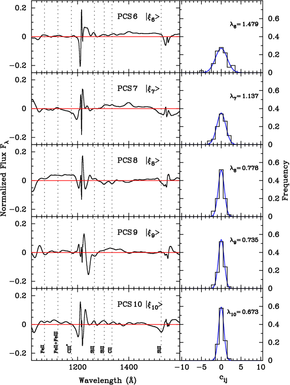
Figure 3: The same as Figure 2 but the second five PCS 6-10. From 8th and higher PCS, the features in PCS become noisy and no longer have physical correspondence. They are probably fitting errors.

Then we wish to use $\lambda_{j}$ to describe the probability distribution function (PDF) of the PCS coefficients. The PDF of the weights is not necessarily a Gaussian, but as shown in Figures 2 and 3, the PDF can be well represented by a Gaussian. We also note that by design:

$$\sum_{i=1}^{N}c_{ij}=0$$ (8)

for any $j$. Thus, the PDF of weights is characterized by just one parameter, $\lambda_{j}$. The probability of having a weight, $c_{ij}$, in an interval, $-x_{0}\leq c_{ij}\leq x_{0}$ can be expressed as:

$$P(-x_{0}\leq c_{ij}\leq x_{0})=\int_{-x_{0}}^{x_{0}}\frac{1}{\sqrt{2\pi}\lambda{j}}e^{-\frac{x^{2}}{2\lambda_{j}^{2}}}dx.$$ (9)

Naturally, it would be convenient if we standardize the weight, $c_{ij}$, by $\lambda_{j}$. We can then rewrite a quasar spectrum as:

$$|q_{i}\rangle\sim|r_{i,m}\rangle=|\mu\rangle+\sum_{j=1}^{m}\lambda_{j}\sigma_{ij}|\xi_{j}\rangle$$ (10)

where the $\sigma_{ij}$ are the standardized PCS coefficients which represent the deviation from the mean spectrum of the $j$th PCS of quasar $i$. The PDF of the $\sigma_{ij}$ is a normal distribution, so we can immediately tell how far and how different the quasar spectrum would be from the mean spectrum. This standardization of the weights simplifies the discussion of the variety of quasar spectra in §5.

Another advantage of using $\lambda_{j}$ is that we can simplify the residual variance fraction f(j):

$$f(j)=\frac{\lambda_{j}^{2}}{\displaystyle\sum_{j=1}^{N}\lambda_{j}^{2}}.$$ (11)

The values of f($j$) are listed in Table 1. The first, second and third PCS account for 63.4%, 14.5% and 6.2% of the variance respectively. In total, the first three PCS account for 84.3% of the variance of the 50 quasars in our sample. These fractions depend on the normalization and the wavelength coverage. In the literature, Francis et al. (1992) report that the first three PCS account for 75% ($\lambda\lambda 1150-2000$), and Shang et al. (2003) show that the first three PCS carry 80% ($\lambda\lambda 1171-2100$) of the variance. Both groups normalized flux by the mean flux, while this paper normalizes by a flux value near 1280 Å. Our value of 84.3% is slightly higher than the above numbers probably because we removed the BAL quasars, which are certainly a source of variance. In addition, we used fitted smooth continua to the Ly$\alpha$ forest, while they used the observed raw Ly$\alpha$ forest which obviously contains a large variance (Tytler et al., 2004a). As shown in Table 1, the contribution from each PCS component to the variance rapidly decreases with order $m$. It becomes less than 1% after the 8th PCS and then stays the same. With seven PCS components, 96% of the variance has already been accounted for. As is seen in the PCS features in Figure 3, the remaining 4% of the variance is probably due to fitting errors.

4 Artificial Spectra

We can use PCS to generate artificial spectra. Artificial spectra can be useful in testing the detection of quasars and DLAs, in flux calibration, in continuum fitting, and in cosmological simulations. By assigning PCS coefficients randomly from known PDFs, we can generate artificial quasar spectra. As we have discussed in §3, the PDF of the $j$th PCS coefficient is well represented by a Gaussian with a mean of 0, and a standard deviation of $\lambda_{j}$. If we then sum up the PCS with these coefficients (equation 10), we can create a set of artificial quasar spectra.

Noiseless quasar spectra are of great use in IGM studies, since at high redshift, it is difficult to see the continuum in the Ly$\alpha$ forest. Even at redshift 2, pixels in the Ly$\alpha$ forest hardly reach the continuum level with FWHM=250km/s (Tytler et al., 2004b). Artificial quasar spectra can thus be useful to predict the shape of continuum in the Ly$\alpha$ forest (Paper I) and to calibrate continuum fitting to the Ly$\alpha$ forest (Tytler et al., 2004a, b). They would be also useful to test the detection limit of the high redshift quasar survey since the Ly$\alpha$ emission can possibly boost the brightness by 0.15 magnitude. We have generated 10,000 artificial quasar spectra using the first seven PCS for a more realistic representation of the quasar spectra. We concluded that the features seen in PCS greater than eighth are noise, and we did not include higher order PCS. We will provide artificially generated spectra to the community upon request.

5 PCA Classification

5.1 Introduction of Five Classes

This paper attempts to classify quasar spectra quantitatively using our standardized PCS coefficients, $\sigma_{ij}$. We note that there is no discrete classification of quasar spectra and that they vary continuously. However, this classification will help us in fitting the continua to the Ly$\alpha$ forest spectrum. We use the first two PCS coefficients to demonstrate the variety of emission lines and continua. As we have seen in §3 and Table 1, the first two PCS coefficients account for 77.9% of the variance and represent the overall shape of the quasar spectrum. We introduce polar coordinates as follows:

$$r_{i} = \sqrt{\sigma_{i1}^{2}+\sigma_{i2}^{2}}$$ (12)

$$\tan\theta_{i} = \frac{\sigma_{i2}}{\sigma_{i1}}$$ (13)

where $r_{i}$ represents the deviation from the mean spectrum, and the angle $\theta_{i}$ tells us about the profiles of the emission lines. We divide the $\sigma_{i1}$ vs. $\sigma_{i2}$ diagram into five zones and introduce five classes of spectral types that enable us to discuss the shape of continua qualitatively. The main goal of this classification is to differentiate the families of quasar spectra. First, we define Class Zero for those close to the mean spectrum in shape. We define Class I-IV corresponding to the quadrant I-IV in the $\sigma_{i1}$ vs. $\sigma_{i2}$ diagram, shown in Figure 4. The probability of $r\leq r_{0}$ is:

$$P(r\leq r_{0}) = \int_{0}^{r_{0}}re^{-\frac{r^{2}}{2}}dr$$ (14)

$$= 1-e^{-\frac{r_{0}^{2}}{2}}.$$ (15)

Now, we wish to design the fraction of the five classes to be equal, namely 0.2 each. We find $r_{0}=0.668$ gives $P(r\leq r_{0})=0.2$, so we define Class Zero for a quasar spectrum that has $r\leq$ 0.668. For quasar spectra with $r>0.668$, we define the classes I through IV corresponding to the quadrants first through fourth on the $\sigma_{i1}$ vs. $\sigma_{i2}$ diagram (Figure 4).

Our standardized PCS coefficients are plotted on the $\sigma_{i1}$ vs. $\sigma_{i2}$ diagram in Figure 4 where the dotted circle is the circle with radius $r_{0}=0.668$. The small numbers noted beside the points are the quasar identification numbers $i$ that are listed in Table 2.

5.2 Demonstration of Five Classes

We show the mean spectrum in Figure 1. By definition the mean spectrum $|\mu\rangle$ has r=0, and naturally it belongs to Class Zero. In Figure 5 we show the artificially generated four classes, I-IV, of the quasar spectra to illustrate their typical spectral shape. They are the sum of the mean and the first two PCS with $\sigma_{i1}=\pm 1$ and $\sigma_{i2}=\pm 1$. The generated four spectra of Class I-IV have angles $\theta$: $45^{\circ},135^{\circ},225^{\circ}$ and $315^{\circ}$ respectively, and they all have $r=\sqrt{2}$. The four spectra are plotted on the same scale in Figure 5 so that we can see the contrast of the emission lines with the continuum in a uniform manner.

In Figure 6-10, we show three observed spectra from each class where we intentionally chose the extreme cases for Class I-IV. Quasars are plotted at rest frame wavelengths with the luminosities that are calculated by using the cosmological parameters from the first year WMAP observation (h=0.71, $\Omega_{m}$=0.27, $\Omega_{\Lambda}$=0.73 ; Spergel et al., 2003), and a flat universe is assumed. The smoothed line on the spectrum is the fitted continuum, and the solid straight line is the power-law continuum fit. The vertical dotted lines show the wavelengths of emission lines in the Ly$\alpha$ forest and the low ionization lines redward of the Ly$\alpha$ emission line. The quasar numbering in Figure 6-10 is the same as in Figure 4 so that we can visualize where the quasar spectrum is in the $\sigma_{i1}$ vs. $\sigma_{i2}$ diagram. In Table 2, quasars are sorted by classes, and the equivalent width of the emission lines are listed.

5.3 The Characteristics of the Five Classes

The characteristics of the first two PCS directly reflect on the five classifications, thus let us take a close look at the first two PCS in Figure 2. The first PCS carries the sharp and strong lines – Ly$\alpha$, Ly$\beta$ and high ionization emission line features (O VI, N V, Si IV, C IV). The second PCS has low ionization emission line features: Fe II and Fe III in blueward of the Ly$\alpha$ emission line, Si II and C II redward. Their profiles are broad and rounded. In the second PCS, the flux values of low ionization emission lines and the strong Ly$\alpha$, C IV emission lines have opposite sign, meaning they are anticorrelated. In addition to that, Ly$\alpha$ and C IV emission lines have P-Cygni profiles which introduces asymmetric profiles to these emission lines.

By definition, the first two PCS engage the correlation between emission lines. Since we are particularly interested in the profiles of emission lines in the Ly$\alpha$ forest, let us look at low ionization lines first. If a quasar shows prominent low ionization lines redward of the Ly$\alpha$ emission line (Si II $\lambda\lambda 1260,1304$, C II $\lambda 1334$), it should have a negative second PCS coefficient, and we should expect to have prominent Fe II $\lambda 1070$ and Fe III $\lambda 1123$ in the Ly$\alpha$ forest. Thus such a quasar should belong to either Class III or IV. As a consequence, these two classes have the largest equivalent widths of these low ionization lines among the five classes as seen in Table 2.

If another quasar has sharp and strong Ly$\alpha$, Ly$\beta$ and high ionization lines (N V, Si IV, C IV), it should have a positive first PCS coefficient and belong to Class I or IV. The normalized flux of the Ly$\alpha$ emission peak and the ratio of the Ly$\alpha$ and N V peak flux are the highest for Class I among the five classes. We can differentiate Class I and II, or Class III and IV by combining the above characteristics. As we expect, the diagonal classes have the opposite characteristics. For example, Class I has sharp and high ionization lines while Class III has broad and rounded low emission lines.

In practice, the key point of finding the continuum level in the Ly$\alpha$ forest is to seek the low ionization lines (Si II $\lambda\lambda 1260,1304$, C II $\lambda 1334$) and their profiles redward of the Ly$\alpha$ emission. If we see them, we should expect to have similar profiles of Fe II $\lambda 1070$ and Fe II $\lambda 1123$ lines in the Ly$\alpha$ forest. If we do not see them, we can expect the continuum to be flat in the Ly$\alpha$ forest, and the power-law extrapolation from the redward of the Ly$\alpha$ emission to be a good approximation. We will discuss the accuracy of the power-law extrapolation in the next section.

6 Mean Flux $\langle F\rangle$ and Flux Decrement D_A

In performing a precise measurement of the IGM flux decrement D_A, it is essential to include the effect of weak emission lines found in the Appendix A. This contribution is not negligible, and will be quantitatively assessed.

6.1 A Brief History of the Flux Decrement D_A

Gunn & Peterson (1965) predicted a flux decrement due to foreground neutral hydrogen in the IGM, namely the Ly$\alpha$ forest. Oke & Korycansky (1982) first defined and measured the flux decrement, D_A. Schneider et al. (1991) introduced the Ly$\alpha$ forest wavelength interval for D_A as $\lambda\lambda 1050-1170$, and it has been widely used since (Zuo & Lu, 1993; Kennefick et al., 1995; Spinrad et al., 1998). Madau (1995) and McDonald & Miralda-Escudé (2001) have used D_A to estimate the UV background. The flux decrement of the high redshift IGM probes the reionization epoch of the universe (Loeb & Barkana, 2001). The current estimate of the reionization epoch from the IGM is around $z\sim 6-7$ (Becker et al., 2001; Djorgovski et al., 2001; Fan et al., 2003), while the first year WMAP satellite estimates $z\sim 20$ (Spergel et al., 2003). The discrepancy is yet to be resolved or explained (Cen, 2003).

A precise measurement of the flux decrement, D_A, is of great importance for studies of the IGM (Rauch, 1998) because it is very sensitive to the cosmological parameters, $\sigma_{8}$ (the amplitude of the mass power spectrum) and $\Omega_{\Lambda}$, as well as to the UV background intensity (Tytler et al., 2004b; Jena et al., 2004). However, it is this sensitivity that makes the D_A measurement a major source of error (Hui et al., 1999; Croft et al., 2002b).

6.2 The Mean Flux Correction Factor $\delta F$

The flux decrement is defined as:

$$D_{A}=1-\int_{1050{\rm\AA}}^{1170{\rm\AA}}\frac{f_{\lambda}(\lambda;Observed)}{f_{\lambda}(\lambda;Continuum)}d\lambda$$ (16)

Thus, what we are measuring is the mean flux:

$$\langle F\rangle=\int_{1050{\rm\AA}}^{1170{\rm\AA}}\frac{f_{\lambda}(\lambda;Observed)}{f_{\lambda}(\lambda;Continuum)}d\lambda$$ (17)

However, the unabsorbed continuum level is not seen in the Ly$\alpha$ forest and the power-law extrapolation from redward of Ly$\alpha$ emission has been used as a continuum. In fact, what is reported in the literature as the mean flux is:

$$\langle F_{Power-Law}\rangle=\int_{1050{\rm\AA}}^{1170{\rm\AA}}\frac{f_{\lambda}(\lambda;Observed)}{f_{\lambda}(\lambda;Power\!-\!Law)}d\lambda$$ (18)

which is not exactly the same as $\langle F\rangle$ since the power-law is a crude approximation of the continuum in the Ly$\alpha$ forest as we have seen in §5, Appendix A, and Figures 6-10. We wish to introduce a correction factor $\delta F$ :

$$\delta F=\int_{1050{\rm\AA}}^{1170{\rm\AA}}\frac{f_{\lambda}(\lambda;Power\!-\!Law)}{f_{\lambda}(\lambda;Continuum)}d\lambda$$ (19)

so that we can estimate the true mean flux $\langle F\rangle$ from the reported mean flux $\langle F_{Power-Law}\rangle$:

$$\langle F\rangle=\langle F_{Power-Law}\rangle\cdot\delta F.$$ (20)

To calculate $\delta F$, we need to find the power-law extrapolation from the redward Ly$\alpha$ emission. Since our wavelength range is limited and not as large as other survey data, it is not as easy to extrapolate. Moreover, we have a series of emission lines, and it is hard to define a continuum level with no emission lines. For example, as shown in Figure 9, Class III quasars have emission lines throughout this wavelength range. However, we have a fitted continuum in the Ly$\alpha$ forest, and we take advantage of it. We choose two points and find a power-law fit which runs through these two points. We choose one from blueward ($\lambda 1100$) and the other from redward ($\lambda 1450$) of the Ly$\alpha$ emission. Then, we can have an inter- and extra-polated power-law continuum and its exponent $\alpha_{\nu}$, for $f_{\nu}\propto\nu^{\alpha_{\nu}}$. The average of $\alpha_{\nu}$ is -0.854 with the standard deviation of 0.507. The power-law continua show that they are all sensible first order approximations which well represent the continua in the Ly$\alpha$ forest. The power-law continua are shown in Figure 6-10.

The calculated $\delta F$ is listed in Table 2 and the average of $\delta F$ is 0.947, with a standard deviation of 0.031. This result means that the power-law approximation misses 5.3% of flux from the quasar in the D_A wavelength range, and proves that the power-law approximation is inadequate to perform a D_A measurement that attempts 1% accuracy (Tytler et al., 2004a; Jena et al., 2004). The distribution of $\delta F$ is shown in Figure 11, and it is not a Gaussian. The PDF of $\delta F$ is asymmetric and has long tail toward small $\delta F$ value.

There are two major reasons for the missing flux. The first reason is that the D_A wavelength range is still in the tail of the prominent Ly$\beta$/O VI and Ly$\alpha$ emission lines. For example, the blueward tail of the Ly$\alpha$ emission starts near $\lambda$1160 which is 10Å below the $\lambda$1170 upper limit of D_A wavelength range. The effect from the tails of Ly$\beta$ and Ly$\alpha$ emission is common for all of the quasars as we can see in Figure 6-10. This contribution is about 4-5%, and we always miss this fraction of the flux, meaning $\delta F$ is always less than unity.

The second reason is the contribution from the weak emission lines in the Ly$\alpha$ forest. The continuum level at the emission lines is naturally above the power-law extrapolation, therefore, we would always expect to miss flux from the emission lines, making $\delta F$ always less than unity. The low ionization emission lines in the Ly$\alpha$ forest are prominent for Class III & Class IV quasars. Four quasars in Class III & Class IV have $\delta F$ less than 0.9, meaning we miss more than 10% of the flux if we use power-law extrapolation. The quasar which has the smallest $\delta F$, 0.86, is Q1544+4855. This quasar is shown on the top panel of Figure 10 and the power-law continuum fit looks sensible. Together with the tails of Ly$\beta$ and Ly$\alpha$ emissions, the low ionization emission lines in the Ly$\alpha$ forest (Fe II, Fe III) contribute 14% of flux which is significant and should not be neglected.

We expect that we need to apply at least a $\delta F$ = 0.947 correction to the D_A measurements in the literature. The discrepancy between the past D_A measurements and Bernardi et al. (2003) using the weak emission profile fitting method is shown in Tytler et al. (2004a, Figure 22). The disagreement is approximately 5% at redshift $2<z<3$, and in terms of the mean flux, the power-law fitted values (Press et al., 1993; Steidel & Sargent, 1987) are always above that of profile fitted ones (Bernardi et al., 2003). The correction factor, $\delta F$ = 0.947, explains this disagreement well.

However, we expect that $\delta F$ changes with redshift, and it is crucial to include the effect from the weak emission lines to investigate the reionization epoch. Known as the Baldwin effect (Baldwin, 1977), the emission profile of lines, such as C IV, and the luminosity of the quasar are correlated. Because of the anticorrelation between equivalent width of C IV and the luminosity, we expect that Class III quasars to be the brightest since they have the smallest C IV equivalent width. Due to the selection effect, we would expect to observe the brightest quasars at high redshifts. Therefore, the fraction of classes for the observed quasars should change with redshift. In fact, the highest redshift quasars reported by Fan et al. (2001), Becker et al. (2001) and Djorgovski et al. (2001) probably belong to Class III, because they all show weak Si II $\lambda 1304$ emission line implying they have weak emission lines in the Ly$\alpha$ forest regain. J104433.04-012502.2 (z=5.80) and J08643.85+005453.3 (z=5.82) definitely belong to Class III since they have broad Ly$\alpha$, N V, and Si II emission lines and low Ly$\alpha$/N V emission intensity ratio. The mean flux correction $\delta F$ of Class III quasars are in the range of 0.91-0.97, meaning the power-law extrapolation misses 3-9% of the flux for Class III quasars. We note that the reported 1-$\sigma$ error of the residual mean flux at redshift z=5.75 by Becker et al. (2001) is 0.03. The contribution from $\delta F$ is bigger than their claimed error, and it is systematic. This correction would bring the observed mean flux down by 3-9% percent and would bring D_A up by the same fraction. Therefore, it is crucial to take into account the $\delta F$ correction in order to investigate the reionization epoch.

7 Summary

We analyzed the wide variety of the emission line profiles in the Ly$\alpha$ forest both in a quantitative and qualitative way. We used PCA to describe the variety of quasar spectra, and we found that 1161 pixels of data ($\lambda\lambda 1020-1600$ with 0.5 Å binning) can be summarized by the primary seven PCS coefficients because the pixels are not independent but are strongly correlated with each other. We presented, for the first time, the idea of generating artificial quasar spectra. Our artificial quasar spectra should be useful in testing the detections, in calibrations, and in simulations. We introduced five classes to differentiate the families of quasar spectra, and showed how the classification can guide us to find the continuum level in the Ly$\alpha$ forest. It is essential to account for emission line features in the Ly$\alpha$ forest to perform a precise measurement of the mean flux in order to probe cosmological parameters, the UV background, and the reionization epoch, otherwise, on average, the commonly used power-law extrapolation continuum misses 5.3% of the flux, and we have cases when it misses up to 14% of the flux.

To investigate the high redshift Ly$\alpha$ forest, we showed the need to account for the emission lines in the Ly$\alpha$ forest. An emission line profile continuum fitting method by Bernardi et al. (2003), or improvement of the PCA method in Paper I would be useful for a large data set such as the Sloan Digital Sky Survey. If we can study the redshift evolution of the quasar spectra and if we can estimate the constituents of classes at a certain redshift, we would be able to estimate the mean flux statistically using the mean flux correction factor $\delta F$. For precision cosmology, the formalized we presented here should play an important role.

I thank Regina Jorgenson, Kim Griest, Jeff Cooke, Carl Melis, Tridi Jena and Geffrey So for their careful reading of this manuscript and encouragnements. I thank David Tytler and David Kirkman for the comments on the manuscript and the discussions on the Ly$\alpha$ forest studies. I thank Art Wolfe and Chris Hawk for the discussions on the emission line identifications. I am grateful to Paul Francis who provided the code and LBQS spectra. Paul Hewett kindly sent the error arrays for those spectra. Wei Zheng and Buell Januzzi kindly provided copies of HST QSO spectra that we used before we located the invaluable collection of HST spectra posted to the web by Jill Bechtold. I thank the Okamura Group at the University of Tokyo from whom I learned the basics of PCA. This work was supported in part by NASA grants NAG5-13113 and HST-AR-10288.01-A from the STScI and by NSF grant AST-0098731.

Appendix A Appendix : Weak Emission Lines in the Ly$\alpha$ Forest

It has been suggested that there exist weak emission lines in the Ly$\alpha$ forest (Zheng et al., 1997; Telfer et al., 2002; Bernardi et al., 2003; Scott et al., 2004), however, their identities, strengths, and line profiles are not well understood. More importantly, we wish to know how they are correlated with other emission lines so that we can predict the strength and profiles of the emission lines in the Ly$\alpha$ forest. We attempt to find the identities of the three weak emission lines in the Ly$\alpha$ forest reported by Tytler et al. (2004b). In this paper, we use their measured wavelengths : $\lambda=1070.95,\lambda=1123.17,\lambda=1175.88$ Å.

A.1 Line at $\lambda=1070.95$ Å : Fe II

Zheng et al. (1997) and Vanden Berk et al. (2001) identified this line as Ar I $\lambda$1066.66, but the contribution from Ar I cannot be this large. The Ar I line has another transition at $\lambda$1048.22 whose transition probability ($A_{ik}$ = $4.94\times 10^{8}s^{-1}$) is stronger than that of $\lambda$1066.66 ($A_{ik}=1.30\times 10^{8}s^{-1}$). However, there is no clear sign of the $\lambda$1048.22 line feature in 50 HST spectra or 79 quasar spectra in Tytler et al. (2004a). In addition, the $\lambda 1070$ line has a broad and asymmetric profile which suggests that this line is a blend of multiple lines. Thus, $\lambda 1070$ is not likely to be a single Ar I line.

Telfer et al. (2002) labeled this $\lambda 1070$ as N II + He II line, and mentioned S IV as a possible candidate. Scott et al. (2004) identify four lines in the proximity of this wavelength : S IV doublet ($\lambda\lambda$1062, 1073) and N II+He II+Ar I ($\lambda$1084). As we have seen in §5, the $\lambda 1070$ line correlates with low ionization lines such as Si II and C II. S IV does not fit into this category. N II seems to be a good candidate, but the N II lines peaks around 1085 Å which is 15 Å away from what we see. It is unlikely that we have 15 Å of wavelength error. For the same reason, He II (1085Å), a high ionization line, is not likely to be the dominant contributor. However, it is reasonable to expect to have an He II line since He II $\lambda$1640 is often seen in quasar spectra. This $\lambda 1070$ line is seen in the Q1009+2956 and Q1243+3047 spectra for which we have high S/N Keck HIRES spectra with a FWHM=0.0285 Å resolution at this wavelength (Burles & Tytler, 1998; Kirkman et al., 2003). If $\lambda 1070$ is comprised of the lines suggested by Scott et al. (2004), we would be able to resolve the individual lines. However, none of the individual emission line are resolved. This fact implies that this emission line is comprised of numerous weak lines and that they are probably low ionization lines because of the good correlation with other low ionization lines.

Fe II suits such a description, and in fact, Fe II has a series of UV transitions around this wavelength range: $\lambda\lambda$1060-1080. However, we don’t see other expected Fe II emission lines. If this $\lambda 1070$ is Fe II, we would expect to see the Fe II UV10 multiplet around $\lambda$1144 , which is supposed to be stronger than the $\lambda 1070$ line. But no sign of an emission line is seen at that wavelength. Therefore, Fe II identification may be wrong or there may be a mechanism that we are not aware of that prevents the expected $\lambda$1144 emission line.

A.2 $\lambda=1123.17$ Å : Fe II + Fe III

Telfer et al. (2002); Vanden Berk et al. (2001) identify $\lambda 1123$ as Fe III. The f-value weighted Fe III UV1 multiplet has a wavelength at 1126.39 Å which is very close to what is observed by Tytler et al. (2004a). The distribution of the multiplet lines matches the broad $\lambda 1123$ feature found in quasars. There are no other major resonance lines in this wavelength range except C I. In the wavelength range $\lambda\lambda 1114-1200$, C I has a series of lines, and there exists stronger lines redward of the Ly$\alpha$ emission line: $\lambda\lambda 1115-1193,\lambda\lambda 1277-1280$. However, we do not see these redward C I emission lines, and there is no sign of correlation between $\lambda 1123$ and these possible lines (Paper I). Thus, $\lambda 1123$ is probably Fe III. In addition to Fe III, Fe II also has UV11-14 multiplets around this wavelength: $\lambda\lambda 1121-1133$. Given the fact that this $\lambda 1123$ line is well correlated with $\lambda 1070$ line, it is reasonable to expect to see Fe II lines here as well, if the identification of $\lambda 1070$ is Fe II.

A.3 $\lambda=1175.88$ Å : CIII^∗

Telfer et al. (2002); Vanden Berk et al. (2001) identified $\lambda 1175$ as C III^∗, although as shown in Table 2, we do not have a clear detection of this line because of it being a weak and narrow feature. We can see the $\lambda 1175$ line in the HST composite spectrum (Telfer et al., 2002), the SDSS composite spectrum (Vanden Berk et al., 2001), and in 11 out of 79 quasar spectra in Tytler et al. (2004a). Therefore, we are confident that this $\lambda 1175$ is a real emission line. The $f-$value weighted wavelength of the C III^∗ line is $\lambda$1175.5289 which matches well the observed wavelength. There is no major resonance line at this wavelength.

A.4 Other Possible Emission Lines in the Ly$\alpha$ Forest

Tytler et al. (2004b) and Telfer et al. (2002) reported observing the Si II $\lambda 1195$ line in their spectra. We do not have any clear detection of the Si II $\lambda$1195 line in the 50 quasar spectra. Since other Si II lines, $\lambda\lambda$1265, 1304, are clearly seen redward of the Ly$\alpha$ emission line, it is plausible to expect the Si II $\lambda$1195 line.

Si III has a transition at $\lambda$1206.50. Since we see both Si II and Si IV redward of Ly$\alpha$ emission, it is natural to expect to see Si III. However, no detection is reported in the literature, and we do not have any positive detection in the 50 quasar spectra. The Si III $\lambda 1206$ emission line is probably too weak or possibly overwhelmed by broad Ly$\alpha$ emission, only 10 Å away, whose equivalent width is often greater than 100Å.

Figure 1: The mean spectrum of 50 HST quasar spectra: The spectrum is normalized near 1280 Å. The wavelengths are taken from Morton (1991) except Fe II, Fe III and CIII^∗ lines that are observed wavelenghs from Tytler et al. (2004b). The tick marks shown below the spectrum are the wavelengths of the Fe II and Fe III multiplet. The dotted line is the power-law continuum apporximation. Note the emission lines do exit in the Ly$\alpha$ wavelength region, We also note the wavelength separation of Si IV doublet at $\lambda$1400 is relatively large, and makes the line profile broad.

Figure 4: The distribution of standardized first two PCS coefficients for 50 quasars. The small number besides each point is quasar number $i$ which is listed in Table 2. For quasars with open circles, we have quasar spectra shown in Figure 6-10. We intentionally chose extreme cases to show a wide variety of quasar spectra. The the dotted circle has the radius of 0.668. We divide this plane into the five zones and define the five classes. We define Class Zero as the quasars which have radius less than or equal to 0.668 and Class I-IV as the ones which have radius greater than 0.668 and are in quadrants I-IV respectively.

Figure 5: The illustration of four classes. We artificially generated these four spectra using the first two PCS. We chose $\pm\sigma_{i1}$ and $\pm\sigma_{i2}$ to generate the four spectra, and equation is given in the legend where $|\mu\rangle$ is the mean spectrum, $\lambda_{1}$ and $\lambda_{2}$ are the square root of the first two eigenvalues, and $|\xi_{1}\rangle$ and $|\xi_{2}\rangle$ are the first two PCS. The wavelengths of low ionization lines are shown as vertical dotted lines. Note that the four spectra are plotted in the same scale, and the emission line peak contrast with the continuum characterizes the classification. Class I and II do not have any weak emission lines and the power-law continuum fit (smooth dotted line) is a good approximation of the continuum in the Ly$\alpha$ forest while Class III and IV show prominent low emission lines.

Figure 11: The distribution of the mean flux correction factor $\delta F$. The mean is 0.947 with the standard deviation of 0.031. The distribution is asymmetric with long tail toward small $\delta F$ values. Class III and IV quasars have prominent emission lines in the Ly$\alpha$ forest, and tend to have small $\delta F$ values. Two extreme spectra for low $\delta F$ are shown in Figure 9 for Q0959+6927 and Figure 10 for Q1544+4855.

Table 1: Eigenvalue and Residual Variance Fraction

Component : $j$	1	2	3	4	5	6	7	8	9	10
Eigenvalue $\lambda_{j}^{2}$	57.204	12.985	5.528	4.614	2.516	2.189	1.293	0.605	0.541	0.453
$\lambda_{j}$	7.563	3.604	2.351	2.148	1.586	1.479	1.137	0.778	0.735	0.673
Residual Variance Fraction f($j$)	0.637	0.145	0.062	0.051	0.028	0.024	0.014	0.007	0.006	0.005
Cummulative Residual Variance Fraction	0.637	0.781	0.843	0.894	0.922	0.947	0.961	0.968	0.974	0.979

Note. — Cummulative residual variance fracion is a simple sum of residual variance fraction upto $j$th PCS.

Table 2: The mean flux correction factor $\delta F$ and equivalent width of emission lines

$i$	Quasar	$\delta$F	Ly$\beta$/OVI	Fe II	Fe III	C III∗	Ly$\alpha$	N V	Si II	Si II	C II	Si IV	C IV
			1025	1071	1123	1176	1216	1240	1263	1307	1335	1397	1549
			(Å)	(Å)	(Å)	(Å)	(Å)	(Å)	(Å)	(Å)	(Å)	(Å)	(Å)
	Class Zero
13	Q0947+3940	0.972	8.8	1.4	0.0	0.0	102.9	0.7	0.5	0.0	0.0	13.2	59.8
25	Q1229-0207	0.953	9.5	0.9	0.2	0.0	87.7	0.4	0.1	1.8	0.0	6.9	47.4
34	Q1424-1150	0.903	9.5	1.1	0.0	0.0	131.9	0.6	0.0	0.0	0.0	8.1	50.4
37	Q1538+4745	0.926	8.2	0.4	0.9	0.0	132.9	0.0	0.0	0.4	0.0	6.8	43.4
48	Q2340-0339	0.963	5.1	0.3	0.0	0.0	83.5	0.7	0.0	0.0	0.0	5.7	41.5
	Average	0.944	8.2	0.8	0.2	0.0	107.8	0.5	0.1	0.4	0.0	8.1	48.5
	STD	0.028	1.8	0.5	0.4	0.0	23.6	0.3	0.2	0.8	0.0	2.9	7.2
	Class I
1	Q0003+1553	0.940	8.6	0.1	0.0	0.0	115.7	0.0	0.0	2.2	0.0	6.5	55.2
8	Q0439-4319	0.970	13.3	0.0	0.0	0.0	119.2	1.1	0.0	1.2	0.0	7.3	58.0
11	Q0637-7513	0.980	15.6	2.5	0.0	0.0	87.2	2.2	0.3	0.0	0.0	8.6	38.9
14	Q0953+4129	0.937	12.1	1.9	0.3	0.0	124.2	1.4	0.3	0.0	0.0	10.6	63.6
18	Q1007+4147	0.943	11.6	2.0	0.1	0.1	145.4	1.9	0.0	2.0	0.3	10.4	65.5
22	Q1137+6604	0.939	10.8	1.8	0.2	0.0	99.2	0.6	0.2	0.6	0.0	7.3	45.1
24	Q1216+0655	0.959	9.9	0.9	0.0	0.0	124.7	0.0	0.0	0.6	0.0	8.8	52.4
32	Q1354+1933	0.974	10.3	0.2	0.1	0.1	134.6	0.5	0.5	2.0	1.1	7.9	65.5
39	Q1622+2352	0.971	9.3	0.7	0.0	0.1	111.3	0.2	0.0	0.0	0.0	7.7	65.2
41	Q1821+6419	0.986	13.6	0.3	0.0	0.0	115.3	0.2	0.0	0.0	0.0	7.8	50.6
42	Q1928+7351	0.982	10.2	0.0	0.0	0.0	149.4	1.9	0.0	0.0	0.0	12.4	74.3
45	Q2243-1222	0.966	8.1	0.3	0.0	0.1	103.2	0.0	0.0	2.2	0.2	8.1	51.6
49	Q2344+0914	0.963	13.9	0.8	0.0	0.0	143.1	1.8	0.5	1.6	0.0	5.3	50.9
	Average	0.962	11.3	0.9	0.1	0.0	121.0	0.9	0.1	1.0	0.1	8.4	56.7
	STD	0.017	2.3	0.9	0.1	0.0	18.7	0.8	0.2	0.9	0.3	1.9	9.8
	Class II
2	Q0026+1259	0.950	9.6	2.4	0.1	0.0	92.1	3.6	0.1	0.0	0.0	9.2	19.4
4	Q0159-1147	0.948	2.8	0.3	0.9	0.0	52.8	1.0	0.0	1.1	0.8	4.2	16.8
5	Q0349-1438	0.974	1.8	0.0	0.0	0.1	54.9	0.0	0.0	0.0	0.0	4.0	28.0
6	Q0405-1219	0.950	6.9	0.7	1.1	0.0	92.5	0.4	0.0	1.1	0.0	6.5	35.0
7	Q0414-0601	0.958	6.1	0.0	0.1	0.0	114.0	0.9	0.0	0.0	0.0	5.1	40.1
9	Q0454-2203	0.935	11.6	4.2	0.0	0.0	105.7	2.2	0.3	1.1	0.0	7.2	33.9
12	Q0923+3915	0.973	7.2	0.0	0.1	0.0	95.1	0.1	0.0	1.2	0.0	5.1	46.4
15	Q0954+5537	0.983	3.3	0.0	0.4	0.1	42.6	0.3	1.1	0.0	0.0	1.9	17.9
20	Q1104+1644	0.958	5.7	0.7	0.0	0.0	104.5	0.0	0.0	0.5	0.0	7.8	54.1
27	Q1252+1157	0.939	6.1	2.7	2.4	0.0	72.7	1.0	0.2	0.0	0.5	6.0	25.5
40	Q1637+5726	0.945	4.5	0.9	0.2	0.0	77.6	0.7	0.0	0.3	0.0	5.4	33.2
47	Q2251+1552	1.015	7.1	2.3	0.0	0.0	60.1	1.0	0.0	0.0	0.0	2.6	23.2
	Average	0.960	6.1	1.2	0.4	0.0	80.4	0.9	0.1	0.4	0.1	5.4	31.1
	STD	0.022	2.8	1.4	0.7	0.0	23.7	1.0	0.3	0.5	0.2	2.1	11.6
	Class III
16	Q0959+6827	0.865	3.6	4.0	2.9	0.1	81.0	3.1	0.7	1.3	1.3	12.1	25.2
17	Q1001+2910	0.949	3.4	3.4	2.4	0.0	68.7	2.0	0.7	2.9	2.1	9.3	26.2
21	Q1115+4042	0.957	7.3	4.3	3.2	0.0	82.3	1.8	0.3	2.5	1.5	8.6	29.7
23	Q1148+5454	0.928	3.4	3.9	2.8	0.0	108.4	1.1	0.9	1.8	1.5	14.1	30.8
26	Q1248+4007	0.937	2.9	3.0	3.2	0.1	111.6	2.1	0.6	1.6	0.6	12.2	28.6
28	Q1259+5918	0.954	2.8	2.5	1.8	0.0	63.5	1.0	1.7	2.7	0.7	10.1	19.8
29	Q1317+2743	0.963	3.2	0.8	1.3	0.0	57.2	1.5	0.4	0.5	0.1	7.1	17.9
30	Q1320+2925	0.977	1.1	3.9	1.2	0.0	58.6	1.0	0.6	0.4	0.1	5.7	14.4
36	Q1444+4047	0.925	4.0	3.0	3.8	0.1	65.0	3.6	0.0	0.3	0.7	9.9	24.0
43	Q2145+0643	0.943	1.6	0.0	0.0	0.0	71.3	0.6	0.0	0.0	0.3	1.6	35.9
44	Q2201+3131	0.928	4.8	0.6	1.2	0.0	69.9	0.0	0.0	0.0	0.0	7.6	28.8
	Average	0.939	3.5	2.7	2.2	0.0	76.1	1.6	0.5	1.3	0.8	8.9	25.6
	STD	0.029	1.6	1.5	1.1	0.0	18.5	1.1	0.5	1.1	0.7	3.5	6.2
	Class IV
3	Q0044+0303	0.965	8.6	1.3	0.0	0.0	146.0	1.5	0.1	1.7	0.1	11.3	71.2
10	Q0624+6907	0.888	8.2	5.1	3.0	0.0	174.5	3.9	0.6	2.5	1.3	11.3	51.7
19	Q1100+7715	0.948	9.7	1.7	0.0	0.0	101.8	1.0	0.0	0.0	0.0	8.5	72.1
31	Q1322+6557	0.925	8.3	1.8	1.7	0.0	138.5	2.7	0.0	3.3	0.8	9.3	55.5
33	Q1402+2609	0.865	6.3	3.1	4.7	0.0	82.0	1.8	0.8	2.3	1.8	5.1	31.7
35	Q1427+4800	0.944	13.9	1.8	0.1	0.0	96.9	0.7	0.0	0.6	0.2	16.9	57.3
38	Q1544+4855	0.860	2.9	5.7	5.5	0.0	119.5	1.0	1.6	5.1	3.6	16.5	33.5
46	Q2251+1120	0.937	10.5	0.8	0.0	0.1	141.6	4.5	0.0	2.1	0.0	7.8	69.8
50	Q2352-3414	0.937	9.0	0.8	1.3	0.0	129.4	0.4	0.0	0.7	0.2	6.6	61.8
	Average	0.919	8.6	2.4	1.8	0.0	125.6	1.9	0.3	2.0	0.9	10.4	56.1
	STD	0.038	3.0	1.8	2.1	0.0	28.7	1.5	0.6	1.6	1.2	4.1	15.1
	Total
	Average	0.947	7.5	1.6	0.9	0.0	100.9	1.2	0.3	1.0	0.4	8.1	42.8
	STD	0.031	3.7	1.5	1.4	0.0	30.4	1.1	0.4	1.1	0.7	3.3	17.0

References

- Bahcall et al. (1993) Bahcall et al. 1993, ApJS, 87, 1
- Bahcall et al. (1996) —. 1996, ApJ, 457, 19
- Baldwin (1977) Baldwin, J. A. 1977, ApJ, 214, 679
- Bechtold et al. (2002) Bechtold et al. 2002, ApJS, 140, 143
- Becker et al. (2001) Becker et al. 2001, AJ, 122, 2850
- Bernardi et al. (2003) Bernardi et al. 2003, AJ, 125, 32
- Boroson (2002) Boroson, T. A. 2002, ApJ, 565, 78
- Boroson & Green (1992) Boroson, T. A. & Green, R. F. 1992, ApJS, 80, 109
- Burles & Tytler (1998) Burles, S. & Tytler, D. 1998, ApJ, 507, 732
- Cabanac et al. (2002) Cabanac, R. A., de Lapparent, V., & Hickson, P. 2002, A&A, 389, 1090
- Cen (2003) Cen, R. 2003, ApJ, 591, 12
- Croft et al. (2002a) Croft, R. A. C., Hernquist, L., Springel, V., Westover, M., & White, M. 2002a, ApJ, 580, 634
- Croft et al. (2002b) Croft, R. A. C., Weinberg, D. H., Bolte, M., Burles, S., Hernquist, L., Katz, N., Kirkman, D., & Tytler, D. 2002b, ApJ, 581, 20
- Djorgovski et al. (2001) Djorgovski, S. G., Castro, S., Stern, D., & Mahabal, A. A. 2001, ApJ, 560, L5
- Fan et al. (2001) Fan et al. 2001, AJ, 122, 2833
- Fan et al. (2003) Fan et al. 2003, AJ, 125, 1649
- Francis et al. (1992) Francis, P. J., Hewett, P. C., Foltz, C. B., & Chaffee, F. H. 1992, ApJ, 398, 476
- Gunn & Peterson (1965) Gunn, J. E. & Peterson, B. A. 1965, ApJ, 142, 1633
- Hewett et al. (1995) Hewett, P. C., Foltz, C. B., & Chaffee, F. H. 1995, AJ, 109, 1498
- Hewett et al. (2001) —. 2001, AJ, 122, 518
- Hui et al. (1999) Hui, L., Stebbins, A., & Burles, S. 1999, ApJ, 511, L5
- Jannuzi et al. (1996) Jannuzi et al. 1996, ApJ, 470, L11
- Jena et al. (2004) Jena, T., Norman, M. L., Tytler, D., Kirkman, D., Suzuki, N., Chapman, A., Melis, C., So, G., O’Shea, B. W., Lin, W., Lubin, D., Paschos, P., Reimers, D., Janknecht, E., & Fechner, C. 2004, MNRASsubmitted, astro-ph/0412557
- Kennefick et al. (1995) Kennefick, J. D., Djorgovski, S. G., & de Carvalho, R. R. 1995, AJ, 110, 2553
- Kirkman et al. (2003) Kirkman, D., Tytler, D., Suzuki, N., O’Meara, J. M., & Lubin, D. 2003, ApJS, 149, 1
- Loeb & Barkana (2001) Loeb, A. & Barkana, R. 2001, ARA&A, 39, 19
- Madau (1995) Madau, P. 1995, ApJ, 441, 18
- McDonald & Miralda-Escudé (2001) McDonald, P. & Miralda-Escudé, J. 2001, ApJ, 549, L11
- Morton (1991) Morton, D. C. 1991, ApJS, 77, 119
- Oke & Korycansky (1982) Oke, J. B. & Korycansky, D. G. 1982, ApJ, 255, 11
- Press et al. (1993) Press, W. H., Rybicki, G. B., & Schneider, D. P. 1993, ApJ, 414, 64
- Rauch (1998) Rauch, M. 1998, ARA&A, 36, 267
- Schneider et al. (1991) Schneider, D. P., Schmidt, M., & Gunn, J. E. 1991, AJ, 101, 2004
- Scott et al. (2004) Scott et al. 2004, ApJ, 615, 135
- Shang et al. (2003) Shang, Z., Wills, B. J., Robinson, E. L., Wills, D., Laor, A., Xie, B., & Yuan, J. 2003, ApJ, 586, 52
- Spergel et al. (2003) Spergel et al. 2003, ApJS, 148, 175
- Spinrad et al. (1998) Spinrad et al. 1998, AJ, 116, 2617
- Steidel & Sargent (1987) Steidel, C. C. & Sargent, W. L. W. 1987, ApJ, 313, 171
- Suzuki et al. (2003) Suzuki, N., Tytler, D., Kirkman, D., O’Meara, J. M., & Lubin, D. 2003, PASP, 115, 1050
- Suzuki et al. (2005) —. 2005, ApJ, 618, 592
- Telfer et al. (2002) Telfer, R. C., Zheng, W., Kriss, G. A., & Davidsen, A. F. 2002, ApJ, 565, 773
- Tytler et al. (2004a) Tytler, D., Kirkman, D., O’Meara, J. M., Suzuki, N., Orin, A., Lubin, D., Paschos, P., Jena, T., Lin, W., Norman, M. L., & Meiksin, A. 2004a, ApJ, 617, 1
- Tytler et al. (2004b) Tytler, D., O’Meara, J. M., Suzuki, N., Kirkman, D., Lubin, D., & Orin, A. 2004b, AJ, 128, 1058
- Vanden Berk et al. (2001) Vanden Berk et al. 2001, AJ, 122, 549
- Yip et al. (2004) Yip et al. 2004, AJ, 128, 2603
- Zheng et al. (1997) Zheng, W., Kriss, G. A., Telfer, R. C., Grimes, J. P., & Davidsen, A. F. 1997, ApJ, 475, 469
- Zuo & Lu (1993) Zuo, L. & Lu, L. 1993, ApJ, 418, 601