What will anisotropies in the clustering pattern in redshifted 21 cm maps tell us?

Abstract

The clustering pattern in high redshift HI maps is expected to be anisotropic due to two distinct reasons, the Alcock-Paczynski effect and the peculiar velocities, both of which are sensitive to the cosmological parameters. The signal is also expected to be sensitive to the details of the HI distribution at the epoch when the radiation originated. We use simple models for the HI distribution at the epoch of reionizaation and the post-reionization era to investigate exactly what we hope to learn from future observations of the anisotropy pattern in HI maps. We find that such observations will probably tell us more about the HI distribution than about the background cosmological model. Assuming that reionization can be described by spherical, ionized bubbles all of the same size with their centers possibly being biased with respect to the dark matter, we find that the anisotropy pattern at small angles is expected to have a bump at the characteristic angular size of the individual bubbles whereas the large scale anisotropy pattern will reflect the size and the bias of the bubbles. The anisotropy also depends on the background cosmological parameters, but the dependence is much weaker. Under the assumption that the HI in the post-reionization era traces the dark matter with a possible bias, we find that changing the bias and changing the background cosmology has similar effects on the anisotropy pattern. Combining observations of the anisotropy with independent estimates of the bias, possibly from the bi-spectrum, may allow these observations to constrain cosmological parameters.

1 Introduction

Observations of redshifted 21 cm radiation from the large-scale distribution of neutral hydrogen (HI) are perceived one of the most important future probes of the universe at high redshifts, and there currently are several initiatives underway towards carrying out such observations. To list a few, the GMRT (, 1991) is already functioning at several bands in the frequency range $150$ to $1420\,{\rm MHz}$, while LOFAR, PST and SKA are in different stages of design and/or construction. These observations hold the potential of probing the HI evolution through epochs starting from the present all the way to $z\sim 50$ when the universe was in the Dark Ages (Miralda-Escude, 2003). Variations with angle and with frequency (or redshift) of the redshifted 21 cm radiation brightness temperature give three dimensional maps of the HI distribution at high $z$ (Hogan & Rees, 1979). The signal is sensitive to the spin temperature $T_{s}$ of the HI hyperfine transition, and at any $z$ the HI will be observed in emission or absorption depending on whether $T_{s}$ is larger or smaller than $T_{\gamma}$ the CMBR temperature. To get a picture of the expected signal, we outline below how $T_{s}$ evolves with $z$.

The evolution of $T_{s}$ is governed by two tendencies, once which drives it towards $T_{\gamma}$ and another towards $T_{g}$ the HI gas kinetic temperature. $T_{s}$ couples to $T_{\gamma}$ through a radiative transition, and it couples to $T_{g}$ through atomic collisions and through the absorption and re-emission of Ly-$\alpha$ photons (the Wouthuysen -Field effect, Wouthuysen 1952,Field 1958 ). The collisional process dominates at high densities where it causes $T_{s}$ to closely follow $T_{g}$. The small density of free electrons, residual after hydrogen recombination at $z\sim 1000$, transfers energy from the CMBR to the gas and maintains $T_{s}=T_{g}=T_{\gamma}$ up to $z\sim 200$. The heat transfer is ineffective at $z<200$, and the HI cools adiabatically whereby $T_{s}=T_{g}<T_{\gamma}$. The collisional process which maintains $T_{s}=T_{g}$ looses out to the radiative process at $z<30$ and $T_{s}$ approaches $T_{\gamma}$. Thus, there is a redshift range $200\geq z\geq 30$ where $T_{s}<T_{\gamma}$ and the HI will be seen in absorption against the CMBR (Scott & Rees, 1990). The HI at these epochs largely traces the dark matter, and the HI maps would probe the power-spectrum of density perturbations at a high level of precision (Loeb & Zaldarriaga 2004; Bharadwaj & Ali 2004a). The first luminous objects, formed at $z\sim 30$, would heat the gas through the emission of soft X-ray photons (Chen & Miralda-Escude 2004; Ricotti & Ostriker 2004 )and through Ly-$\alpha$ photons which would also couple $T_{s}$ to $T_{g}$ through the Wouthuysen -Field effect. The HI gas will now be partially heated , and the coupling of $T_{s}$ to $T_{g}$ will also be partial depending on the local flux of Ly-$\alpha$ photons. This is an additional source of fluctuation in the HI maps, and it may be possible to detect the presence of the first luminous objects in the redshift range $30\leq z\leq 15$ through this effect (Barkana & Loeb 2004a, 2004b). The coupling of $T_{s}$ to $T_{g}$ is expected to be saturated by $z\sim 15$, and $T_{s}=T_{g}\gg T_{\gamma}$ throughout the gas ie. the HI will be seen in emission and the HI maps will again trace the dark matter. This changes at $z\sim 10$ when a substantial fraction of the HI is ionized by the first luminous objects. During the epoch of reionization, the HI maps trace the size, shape and topology of the ionized regions (Gnedin 2000; Ciardi et al. 2003; Sokasian et al. 2003a, 2003b; Furlanetto , Zaldarriaga & Hernquist 2004a, 2004b). At low redshifts ($z<6$), the bulk of the HI is in the high column density clouds seen as DLAs in quasar spectra (Péroux et al. 2001; 1996; Lanzetta , Wolfe & syosiTurnshek 1998). These clouds are possibly disk galaxies or their progenitors, and they trace the dark matter, may be with some bias. The HI will be seen in emission, and the maps will trace the dark matter (Bharadwaj , Nath & Sethi 2001; Bharadwaj & Srikant 2004).

Though the HI signal in each redshift range will probe a different phase of the HI evolution and have it’s own distinct signature, there is one thing in common throughout in that the clustering pattern will be anisotropic. The anisotropies in the clustering pattern are the results of two distinct effects. The first is the Alcock-Paczynski effect (Alcock & Paczynski 1979, hereafter the AP effect) caused by the non Euclidean geometry of space time and the second is the effect of peculiar velocities. The AP effect causes objects which are intrinsically spherical in real space to appear elongated along the line of sight in redshift space. This effect is particularly important at high redshifts ($\rm z\geq.1$) where it is sensitive to the cosmological parameters which it can be used to probe. The two-point correlation function of the gravitational clustering of different kinds of objects is expected to be statistically isotropic, and this is a natural choice for applying this test. Galaxy redshift surveys do not extend to sufficiently high redshifts for this effect to be significant. Quasar redshift surveys extend to much higher redshifts and there has been a considerable amount of work (eg. Ballinger , Peacock , & Heavens 1996 , Matsubara & Suto 1996 , Nakamura , Matsubara , & Suto 1998 , Popowski et al. 1998 ,Nair 1999) investigating the possibility of determining the parameters $\Omega_{m}$ and $\Omega_{\Lambda}$. The main problem is that quasar surveys (eg. SDSS) are very sparse and hence they are not optimal for determining the cosmological parameters (Matsubara & Szalay 2002). Hui & Haiman (2003) have used the AP test to constrain cosmological parameters using the Lyman-alpha forest.

The redshift, used to infer radial distances, has a contribution from the line of sight component of the peculiar velocity and this introduces a preferred direction in the redshift space clustering pattern. There are two characteristic effects of peculiar velocities. On small scales, the random motions in virialized regions causes the clustering pattern to appear elongated along the line of sight in redshift space. On large scales the coherent infall onto clusters and superclusters, and the outflow from voids causes the redshift space clustering pattern to appear compressed along the line of sight (the Kaiser effect, Kaiser 1987). This effect can be modeled using linear theory and the anisotropies in the redshift space clustering pattern can be used to determine the parameter $\beta=\Omega_{m}^{0.6}/b$ where $\Omega_{m}$ and $b$ are the cosmic mass density parameter and the linear bias parameter respectively (Kaiser 1987, Hamilton 1992). The Kaiser effect has been studied in the different large galaxy redshift surveys (eg. SDSS , 2dfGRS) and a recent investigation of the redshift space distortions in the 2dFGRS yields a value of $\beta=0.49\pm 0.09$ (Hawkins et al. 2002) at an effective redshift $z\approx 0.15$ .

Future redshift survey carried out using redshifted 21 cm HI radiation will allow the anisotropies arising from both the AP effect and the peculiar velocities to be studied to redshifts as high as $z\sim 50$ and possibly higher, surpassing the potential of any future galaxy or quasar survey. In a recent paper Nusser (2004) has studied the AP effect in redshifted 21 cm maps of the epoch of reionization and he has proposed that a determination of the correlation of temperature fluctuations to an accuracy of $20\%$ should allow a successful application of the AP test to constrain the background cosmological model.

Barkana & Loeb (2004a) have proposed that measuring the anisotropy of the HI power spectrum arising from peculiar velocities provides a means for distinguishing between the different sources which contribute to HI fluctuations. Further, they propose that it may be possible to separate the primordial inflationary power spectrum imprinted in the dark matter from the various astrophysical sources which will also contribute to the HI fluctuations.

In this paper we re-examine exactly what we hope to learn from observations of the anisotropy in HI maps. The previous analysis of Barkana & Loeb (2004a) using the power spectrum implicitly assumes that the background cosmological model is known to a great level of precision and hence does not take into account the anisotropies introduced by the geometry (AP effect). We adopt a framework which allows high redshift HI observations to be interpreted without reference to a background cosmological model. We use the HI temperature two-point correlation function which deals with directly observeable quantities. Using this framework, we quantify the anisotropy and study its dependence on the background cosmological model. The AP effect and the Kaiser effect differ in their response to variations in the background cosmological model. To estimate the relative contributions from these two effect we also calculate the anisotropy ignoring the peculiar velocities.

Our work focuses on the signal expected from the epoch of reionization and the post re-ionization era, these being the most promising frequency bands for observations in the near future. The HI distribution in these eras is largely unknown, and it is expected to differ from the dark matter distribution. The HI is expected to have a very patchy distribution at epoch of reionization. Determining the size, shape and distribution of the ionized regions is one of the main forces driving the effort towards future HI observations. The post-reionization HI will probably trace the dark matter with a bias. In addition the parameters of the background cosmological model, the anisotropy in the HI maps is expected to also be sensitive to the details of the high redshift HI distribution, the latter being largely unknown. In this paper we use simple models for the HI distribution to ask if observations of the anisotropy tell us more about the background cosmological models or the details of the HI fluctuations.

This paper is organized as follow. In Section 2. we explain the origin of the anisotropies and how they can be quantified. In Section 3. we present the background cosmological models and models for the HI distribution. Section 4 contains the results and in Section 5. we present discussion and conclusions.

It may be noted that unless mentioned otherwise, we use the values $(\Omega_{b}h^{2},h)=(0.02,0.7)$ throughout.

2 Origin of the anisotropies

Observations of the HI radiation at a redshift $z$ along the direction of the unit vector ${\bf m}$ will measure

$$\delta T_{b}({\bf m},z)=\frac{T_{b}({\bf m},z)-T_{\gamma}}{1+z}\,,$$ (1)

$T_{b}(z,{\bf m})$ being the brightness temperature of the HI radiation at the position and epoch when the radiation originated and $T_{\gamma}$ the temperature of the CMBR also at the same epoch. It is convenient to represent such observations as $\delta T_{b}({\bf z})$ where ${\bf z}=z\,{\bf m}$ denotes the space of possible redshifts and directions of observation which we refer to as redshift space. Here we assume that the redshift range and region of the sky under observation are both small. Under this assumption, the separation between any two points in redshift space is

$${\bf\Delta z}=\Delta z\,{\bf n}+z\vec{\theta_{\perp}}$$ (2)

where ${\bf n}$ is the line of sight to the center of the region being observed, $z$ is the mean redshift, $\Delta z$ the difference in redshift and $\vec{\theta}$ is the angular separation which is a two dimensional vector in the plane of the sky. It may be noted that $\Delta z\,{\bf n}$ and $z\vec{\theta_{\perp}}$ are respectively the components of ${\bf\Delta z}$ parallel and perpendicular to the line of sight ${\bf n}$, and we introduce the notation $\theta_{\parallel}=\delta z/z$ whereby

$${\bf\Delta z}=z\,(\theta_{\parallel}\,{\bf n}+\vec{\theta_{\perp}})$$ (3)

We next shift our attention to quantifying the fluctuations in the HI brightness temperature. The temperature two point correlation function

$$w(\theta_{\parallel},\theta_{\perp})=\langle\delta T_{b}({\bf z})\,\delta T_{b}({\bf z+\Delta z})\rangle$$ (4)

is the statistical quantity of our choice. Here we have invoked the property of statistical isotropy whereby $w$ is independent of the direction of $\vec{\theta_{\perp}}$. The point to note is that $w(\theta_{\parallel},\theta_{\perp})$ characterizes the observations solely in terms of directly observable quantities, namely angles and redshifts. and does not refer to a background cosmological model. It is necessary to assume a cosmological model in order to assign a physical position ${\bf r}$ to a vector ${\bf z}$ in redshift space. Using $r(z)$ to denote the comoving distance corresponding to a redshift $z$,

$$r(z)=\int^{0}_{z}\frac{c\,dz^{{}^{\prime}}}{H(z^{{}^{\prime}})}$$ (5)

where $H(z)$ is the Hubble parameter, we can assign the vector ${\bf r}=r(z)\,{\bf m}$ in real space to the vector ${\bf z}=z\,{\bf m}$ in redshift space. The physical separation ${\bf\Delta r}$ (in comoving coordinates) corresponding to the separation ${\bf\Delta z}$ in eq. (3) is

$${\bf\Delta r}=r(z)\,\left[p(z)\,\theta_{\parallel}\,{\bf n}+\vec{\theta_{\perp}})\right]$$ (6)

where $p(z)=d\ln r(z)/d\ln z$. The presence of the term $p(z)$ in eq. (6) makes the mapping from redshift space to real space anisotropic when $p(z)\neq 1$. At low redshifts $(z\ll 1)$ we have $r=cz/H_{0}$ whereby $p(z)=1$ and ${\bf\Delta r}=(c/H_{0})\,{\bf\Delta z}$ ie. the mapping from redshift to real space is isotropic. The high redshift behaviour of $p(z)$ depends on the cosmological model (Figure 1) with the feature $p(z)<1$ being common to all the models. This introduces an anisotropy, and a sphere ${(\bf\Delta r})^{2}=R^{2}$ in real space will appear as an ellipsoid $(\theta_{\parallel}\,p)^{2}+(\vec{\theta_{\perp}})^{2}=(R/r)^{2}$ elongated along the line of sight in redshift space. This is the Alcock-Paczynski (Alcock & Paczynski, 1979) effect. For a fixed redshift, the elongation depends on the cosmological model. For all models, the elongation increases with $z$.

We next discuss how the AP effect will manifest itself in $w(\theta_{\parallel},\theta_{\perp})$. Assuming for the time being that the fluctuations in the HI brightness temperature directly trace the fluctuations in the HI density at the point where the radiation originated ie. $\delta T_{b}({\bf z})=K\,\delta_{\rm HI}({\bf r})$ we have

$$w(\theta_{\parallel},\theta_{\perp})=K^{2}\,\xi_{\rm HI}({\bf\Delta r},\,z)$$ (7)

where $\delta_{{\rm HI}}$ denotes fluctuations in the HI density, $\xi_{{\rm HI}}({\bf\Delta r})=\langle\delta_{{\rm HI}}({\bf r})\delta_{{\rm HI}}({\bf r+\Delta r})\rangle$ is the two-point correlation function of $\delta_{{\rm HI}}$ and $K$ is a proportionality factor. We expect the fluctuations in the HI density to be statistically isotropic ie. $\xi_{{\rm HI}}$ will not depend on the direction of ${\bf\Delta r}$. It then follows from the preceding discussion that $w(\theta_{\parallel},\theta_{\perp})$ will be anisotropic when $p(z)\neq 1$, and the curves of constant $w(\theta_{\parallel},\theta_{\perp})$ will be ellipses elongated along the line of sight.

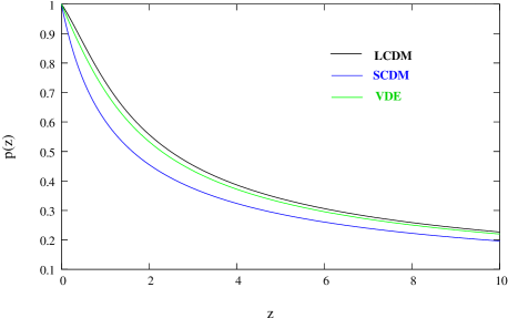
Figure 1: This shows the redshift dependence of the geometrical distortion parameter $p(z)$ for different background cosmological models.

The analysis till now has ignored the effect of peculiar velocities. The line of sight component of the peculiar velocity makes an additional contribution to the redshift, and eq. (5) does not correctly predict the comoving distance. On large scales the peculiar velocity field is well described using linear perturbation theory which relates it to density fluctuations in the underlying dark matter distribution. The coherent flows into over-dense regions and out of under-dense regions leads to the compression of structures along the line of sight (Kaiser, 1987). The introduces an an anisotropy pattern which is opposite in nature to the AP effect.

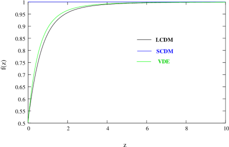
Figure 2: This shows the redshift dependence of the peculiar velocity distortion parameter $f(z)$ for different background cosmological models. It may be noted that for the SCDM model $f(z)=1$ throughout.

Incorporating the effect of the coherent flows to linear order, the fluctuations is the brightness temperature of the HI radiation has been calculated (Bharadwaj & Ali 2004a,Bharadwaj & Ali 2004b) to be

$$\delta T_{b}({\bf z})=\bar{T}(z)\times\eta_{{\rm HI}}({\bf r},z)$$ (8)

where

$$\bar{T}(z)=4.0\,\rm mK(1+z)^{2}\,\left(\frac{\Omega_{b}h^{2}}{0.02}\right)\left(\frac{0.7}{h}\right)\frac{H_{0}}{H(z)}$$ (9)

is the mean brightness temperature of redshifted 21 cm radiation which depends only on $z$ and the background cosmological parameters , and

$$\eta_{{\rm HI}}({\bf r},z)=\frac{\rho_{{\rm HI}}}{\bar{\rho}_{{\rm H}}}\left(1-\frac{T_{\gamma}}{T_{s}}\right)\left[1-\frac{(1+z)}{H(z)}\frac{\partial v}{\partial r}\right]$$ (10)

is the “21 cm radiation efficiency in redshift space”. The term $\eta_{{\rm HI}}({\bf r},z)$ should be evaluated at ${\bf r}$, the position in real space corresponding to ${\bf z}$ - calculated using eq. (5)) without the effect of peculiar velocities, at the epoch corresponding to the redshift $z$. Here the term $\rho_{{\rm HI}}/\bar{\rho}_{{\rm H}}$ is the ratio of the neutral hydrogen density to the mean hydrogen density. Assuming that the hydrogen traces the dark matter and that the neutral fraction varies from place to place we have $\rho_{HI}({\bf r},z)=\bar{\rho}_{H}(z)\,\bar{x}_{HI}(z)[1+\delta_{x}({\bf r},z)][1+\delta({\bf r},z)]$. Here $\delta_{x}$ and $\delta$ refer to fluctuations in the neutral fraction and the dark matter respectively, and $\bar{x}_{HI}$ is the mean neutral fraction. The spin temperature $T_{s}$ also can vary from place to place i .e $T_{s}({\bf x},z)=\bar{T_{s}}(z)[1+\delta_{s}({\bf x},\,z)]$. The last term in eq. (10) incorporates the effects of linear peculiar velocities where $v({\bf r},z)$ is the line of sight component of the peculiar velocity and $\partial v/\partial r$ is its radial derivative. We then have, at linear order, the fluctuating part of $\eta_{{\rm HI}}({\bf r},z)$ to be

$$\eta_{{\rm HI}}({\bf r},z) = \bar{x}_{HI}(z)\left\{\left(1-\frac{T_{\gamma}}{\bar{T_{s}}}\right)\left[\,\delta({\bf r},z)+\delta_{x}({\bf r},z)\right.\right.$$ (11)

$$- \left.\left.\frac{(1+z)}{H(z)}\frac{\partial v({\bf r},z)}{\partial r}\right]+\frac{T_{\gamma}}{\bar{T_{s}}}\,\delta_{s}({\bf r},z)\,\right\}$$

This is most conveniently expressed in Fourier space as

$$\eta_{{\rm HI}}({\bf x},z)=\int\frac{d^{3}k}{(2\pi)^{3}}\,\tilde{\eta}_{\rm HI}({\bf k},z)\,e^{-i\ {\bf k}\cdot{\bf x}}$$ (12)

where

$$\tilde{\eta}_{\rm HI}({\bf k},z) = \bar{x}_{HI}(z){\bigg{\{}}(1-\frac{T_{\gamma}}{T_{s}})\left[\Delta({\bf k},z)+\Delta_{x}({\bf k},z)\right.$$ (13)

$$+ \left.f\mu^{2}\Delta({\bf k},z)\right]+\frac{T_{\gamma}}{T_{s}}\Delta_{s}({\bf k}\,z)\,\,{\Bigg{\}}}$$

Here $\mu={\bf n}\cdot{\bf k}/k$ is the cosine of the angle between the Fourier mode ${\bf k}$ and the line of sight ${\bf n}$ towards the center of the part of the sky under observation, and $f=dlnD/dlna$ where $D(a)$ is the growing mode of density perturbations (Peebles, 1993) and $a$ is the scale factor. The term involving $f\,\mu^{2}$ arises from the peculiar velocities.

The HI correlation function $\xi_{{\rm HI}}({\bf\Delta r},z)=\langle\eta_{{\rm HI}}({\bf r},z)\eta_{{\rm HI}}({\bf r+\Delta r},z)\rangle$ and the HI power spectrum $P_{{\rm HI}}({\bf k},z)$ defined as $\langle\tilde{\eta}_{\rm HI}({\bf k},z){\tilde{\eta}_{\rm HI}}^{*}({\bf k}^{{}^{\prime}},z)\rangle=(2\pi)^{3}\delta^{3}({\bf k}-{\bf k}^{\prime})P_{{\rm HI}}({\bf k},z)$ are related as

$$\xi^{s}_{HI}({\bf\Delta r},z)=\int\frac{d^{3}k}{(2\pi)^{3}}e^{-i\,\bf k\cdot\,{\bf\Delta r}}P_{HI}({\bf k},z).$$ (14)

where the HI power spectrum is

$$P_{HI}({\bf{k}},z) = {\bar{x}}^{2}_{HI}(z)\,{\bigg{\{}}\left(1-\frac{T_{\gamma}}{\bar{T}_{s}}\right)^{2}\,[(1+f\,{\mu}^{2})^{2}\,P_{\delta-\delta}(k,z)$$ (15)

$$+ 2(1+\ f\,{\mu}^{2})\,P_{\delta-x}(k,z)+P_{x-x}(k,z)]\,$$

$$+ 2\left(1-\frac{T_{\gamma}}{\bar{T}_{s}}\right)\,\frac{T_{\gamma}}{\bar{T}_{s}}[(1+f\,{\mu}^{2})\,P_{\delta-s}(,z)$$

$$+ P_{x-s}({\bf{k}},z)]+\left(\frac{T_{\gamma}}{\bar{T}_{s}}\right)^{2}\,P_{s-s}(k,z)\,\,{\Bigg{\}}}$$

Here $P_{\delta-\delta}(k,z)$, $P_{x-x}(k,z)$ and $P_{s-s}(k,z)$ are the power spectra of the three different sources which contribute to the HI fluctuations, the dark matter, neutral fraction and spin temperature fluctuations respectively. The cross power spectra $P_{\delta-x}(k,z)$, $P_{\delta-s}(k,z)$ and $P_{x-s}(k,z)$ quantify cross-correlations, if any, between these different sources. The presence of peculiar velocities makes the HI power spectrum $P_{{\rm HI}}({\bf k},z)$ anisotropic through the terms involving $f\mu^{2}$ which appear in eq. (15). It should be noted that $f\mu^{2}$ appears only with the sources of HI fluctuation that are correlated with the dark matter fluctuations, and the contribution to the HI power spectrum from components not correlated with the dark matter are isotropic.

The anisotropy of $P_{{\rm HI}}({\bf k},z)$ is reflected in $\xi_{{\rm HI}}({\bf\Delta r},z)$ which depends on how ${\bf\Delta r}$ is aligned with respect to ${\bf n}$. Further, $\xi_{{\rm HI}}({\bf\Delta r},z)$ depends only on the even powers of ${\bf n}\cdot{\bf\Delta r}/\Delta r$. Shifting our focus back to $w(\theta_{\parallel},\theta_{\perp})$ we have

$$w(\theta_{\parallel},\theta_{\perp})=\bar{T}^{2}(z)\,.\xi^{s}_{{\rm HI}}({\bf\Delta r},z)$$ (16)

The correlation in the HI brightness temperature fluctuations, $w(\theta_{\parallel},\theta_{\perp})$ is anisotropic due to two reasons, first because the mapping from $(\theta_{\parallel},\theta_{\perp})$ to ${\bf\Delta r}$ is anisotropic (the AP effect) and second because $\xi_{{\rm HI}}$ is intrinsically anisotropic due to the effect of peculiar velocities. Here we investigate whether it will be possible to observationally distinguish these two distinct sources of anisotropy. Both these effects depend on the background cosmological model, and we investigate to what extent observations of the anisotropy can be used to determine the cosmological parameters. Finally, the anisotropy in the HI power spectrum depends on the properties of the different sources which contribute to HI fluctuations. We investigate to what extent observations of anisotropies in the HI can disentangle the contributions from the different sources.

3 Models

3.1 Background Cosmology

We have considered a few representative cosmological models, all of which are spatially flat and have two components namely dark matter and dark energy. The possibility that the dark energy equation of state evolves with time has, of late, received a considerable amount of attention (eg. Peebles & Ratra 1988 , Riess et al. 1998 , Perlmutter et al. 1999 , Sahni & Starobinsky 2000 , Sahni & Wang 2000 , Saini et al. 2000, Carroll 2001, Huterer & Turner 2001, Perlmutter 2003, Linder 2003, Alam et al. 2004 ) . Here we consider a possible parameterization of the variable dark energy (VDE) model introduced by Wang & Tegmark (2004). The Hubble parameter is of the form

$$H(z)=H_{0}\,[\Omega_{m0}\,(1+z)^{3}+(1-\Omega_{m0})f_{DE}(z)]^{1/2}.$$ (17)

where $H_{0}$, $\Omega_{m0}$, and $1-\Omega_{m0}$ are the present values of the Hubble parameter, the dark matter density parameter and the dark energy density parameter respectively, and $f_{DE}(z)=\rho_{DE}(z)/\rho_{DE}(0)=f_{\infty}+(1-f_{\infty})\,\,(1+z)^{3(1+w_{i})}$ is the dimensionless dark energy density function. This VDE model has two extra parameters $f_{\infty}$ and $w_{i}$ compared to the usual LCDM model, and the parameters are restricted to the range $w_{i}\geq-2$ and $f_{\infty}\geq 0$. The VDE model reduces to to LCDM model if either $f_{\infty}=1$ or $w_{i}=-1$. In addition to the SCDM model ($\Omega_{m0}=1$) and the LCDM model with $\Omega_{m0}=0.3$, we have considered the VDE model with $\Omega_{m0}=0.4$ and $(f_{\infty},w_{i})=(1.2,-1.8)$. In the VDE models which we have considered, $f_{DE}(z)$ increases from $f_{DE}(0)=1$ and saturates at $f_{\infty}=1.2$ around $z\sim 3$. The value of $f_{DE}$ reaches the saturation value at a lower redshift is $w_{i}$ is decreased. Figures 1 and 2 show the behavior of $p(z)$ and $f(z)$ respectively for the models considered here. The points to note are (1.) Though in all models $p(z)$ falls rapidly up to $z\sim 5$ beyond which it decreases gradually, the values of $p(z)$ are different in each of the models, and (2.) The values of $f(z)$ differ from model to model only for $z<4$, and $f(z)\sim 1$ at larger redshifts where the universe is dark matter dominated.

3.2 The HI distribution

We focus our attention on two different epochs which we discuss below.

3.2.1 Reionization

We adopt a simple model for the hydrogen distribution where there are spherical ionized bubbles of comoving radius $R$ and the region outside the bubbles is completely neutral. The total hydrogen density is assumed to trace the dark matter distribution. The reionization is believed to have been caused by the first luminous objects which are expected to be highly clustered. We incorporate this by assuming that the centers of the ionized bubbles are biased with respect to the dark matter distribution with a bias $b_{c}$. Further, we assume that the hydrogen has been heated before reionization ie. $T_{s}\gg T_{\gamma}$ and consequently the HI will be observed in emission. The fluctuations in the neutral fraction $(\delta_{x})$ has two parts, one which is correlated with the dark matter fluctuations and another, arising from the discrete nature of the ionized regions, which is uncorrelated with the dark matter distribution. The spin temperature fluctuations $(\delta_{s})$ do not contribute when $T_{s}\gg T_{\gamma}$. The power spectrum for the resulting HI distribution is (Bharadwaj & Ali, 2004b)

$$P_{{\rm HI}}({\bf k},z) = \left[\bar{x}_{{\rm HI}}(1+f\mu^{2})-b_{c}f_{V}W(kR)\right]^{2}P_{\delta-\delta}(k,z)$$ (18)

$$+ \frac{f^{2}_{V}W^{2}(kR)}{\bar{n}_{{\rm HI}}}$$

where $W(y)=(3/y^{3})[\sin(y)-y\cos(y)]$ is the spherical top hat window function, $f_{V}$ is the fraction of volume which is ionized, $\bar{n}_{{\rm HI}}$ is the comoving number density of the spheres and $f_{V}=(1-\bar{x}_{{\rm HI}})=\frac{4}{3}\pi R^{3}\bar{n}_{{\rm HI}}$.

of spherical HII region The first term which contains $P_{\delta-\delta}(k)$ arises from the clustering of the hydrogen and the clustering of the centers of the ionized spheres. The second term which has $1/\bar{n}_{{\rm HI}}$ is the Poisson noise due to the discrete nature of the ionized regions. The latter is not correlated with the dark matter.

This model has a limitation that the HI density is negative in a fraction $\sim f_{V}^{2}/2$ of the total volume where ionized spheres overlap. The possibility of the spheres overlapping increases if they are highly clustered. This restricts the range of $f_{V}$ and $b_{c}$ where this model is meaningful.

3.2.2 Post-reionization

At low redshifts the bulk of the HI is in the high column density clouds which produce the damped Lyman-$\alpha$ absorption lines observed in quasar spectra (Péroux et al. 2001 , 1996 , Lanzetta , Wolfe & syosiTurnshek 1998). These observations currently indicate $\Omega_{gas}(z)$ , the comoving density of neutral gas expressed as a fraction of the present critical density, to be nearly constant at a value $\Omega_{gas}(z)\sim 10^{-3}$ for $z\geq 1$ (Péroux et al., 2001). The damped Lyman-$alpha$ clouds are believed to be associated with galaxies which represent highly non-linear overdensities. It is now generally accepted from the study of the large scale structures in redshift surveys and N-body simulations that the galaxies (or nonlinear structures) are a biased tracer of the underlying dark matter distribution (Kaiser 1984 ;Dekel & Lahav 1999;Mo & White 1996 ;Taruya & Suto 2001 and Yoshikawa et al. 2001). On the large scales of interest here it is reasonable to assume that these HI clouds trace the dark matter with a constant, linear bias $b$.

Converting $\Omega_{gas}$ to the mean neutral fraction $\bar{x}_{{\rm HI}}=\bar{\rho}_{{\rm HI}}/\bar{\rho}{{\rm H}}=\Omega_{gas}/\Omega_{b}$ gives us $\bar{x}_{{\rm HI}}=50\Omega_{gas}h^{2}(0.02/\Omega_{b}h^{2})$ or $\bar{x}_{{\rm HI}}=2.45\times 10^{-2}$. We also assume $T_{s}\gg T_{\gamma}$ and hence we see the HI in emission. Using these we have

$$P_{{\rm HI}}({\bf k},z)=\bar{x}^{2}_{{\rm HI}}\left(1+\beta\mu^{2}\right)^{2}\,P_{\delta-\delta}(k,z)$$ (19)

where $\beta=f/b$. The fact that the neutral hydrogen is in discrete clouds makes a contribution which we do not include here. Another important effect not included here is that the fluctuations become non-linear at low $z$. Both these effects have been studied using simulations (Bharadwaj & Srikant, 2004).

4 Results

We quantify the anisotropies in the HI clustering pattern by decomposing $w(\theta_{\parallel},\theta_{\perp})$ into different spherical harmonics

$$w_{l}{(\theta)}=\frac{2\,l+1}{2}\int^{1}_{-1}w{(\theta,\,\tilde{\mu})}\,\,P_{l}(\tilde{\mu})\,d\tilde{\mu}$$ (20)

where $P_{l}(\tilde{\mu})$ are the Legendre polynomials and we have used $w(\theta,\tilde{\mu})=w(\theta_{\parallel},\theta_{\perp})$ where $\theta=\sqrt{\theta_{\parallel}^{2}+\theta_{\perp}^{2}}$ and $\tilde{\mu}=\theta_{\parallel}/\theta$. The fact that $P_{{\rm HI}}({\bf k},z)$ depends only on even powers of $\mu$ ensures that all the odd harmonics will be zero. In addition to the monopole $w_{0}(\theta)$, we have calculated the quadrupole $w_{2}(\theta)$ and the hexadecapole $w_{4}(\theta)$ and we use the ratios $w_{2}/w_{0}$ and $w_{4}/w_{0}$ to quantify the anisotropies.

4.1 Reionization

We have restricted our analysis to $z=10$ which corresponds to $129\,{\rm MHz}$ and assume that half the hydrogen is ionized at this redshift ie. $f_{V}=0.5$ (Zaldarriaga , Furlanetto & Hernquist, 2004). Recent investigations indicate that at this redshift the comoving size of the ionized bubbles will be of the order of a few ${\rm Mpc}$ (Furlanetto , Zaldarriaga & Hernquist, 2004a). Further, Furlanetto , Zaldarriaga & Hernquist (2004a) also show that the bias is expected to have a low value (near unity) for large bubble size $R$. We consider the LCDM model with $R=3\,h^{-1}{\rm Mpc}$ and $b_{c}=1.5$ as the fiducial model (Model A) for which Figures 3, 4 and 5 show $w_{0}$, $w_{2}/w_{0}$ and $w_{4}/w_{2}$ respectively. To study how the signal depends on various factors, we have varied the background cosmological model and the parameters $R$ and $b_{c}$. Further, we have also considered the signal without the effect of the peculiar velocities and the Poisson term in order to explicitly isolate the contribution from these terms. Table 1 shows the various combinations for which we have calculated the expected signal.

One of the salient features of the monopole $w_{0}$ (Figure 3) is that the signal is dominated by the Poisson fluctuations from the discrete ionized bubbles on small scales whereas it traces the dark matter on large scales. The angular scale where the transition from Poisson fluctuations to dark matter occurs depends on the background cosmological model. Further, the Poisson contribution increases if the bubbles are larger (increasing $R$) because the number density of bubbles falls. The dependence on the background cosmological model can be attributed to the fact that the comoving distance corresponding to $z=10$ differs by around $10\%$ in the LCDM and VDE models whereby the same ionized bubbles correspond to different angles in the two models. It should be noted that though the overall amplitude of $w_{0}$ also changes with the background cosmological model, it would not be possible to distinguish this from a change in the neutral fraction which would have the same effect. Increasing $b_{c}$ increases the overall-amplitude of the signal at large scales leaving it unchanged at very small scales. The effect of peculiar velocities, we find, depends on the value of $b_{c}$, and it increases the signal when $b_{c}=0$ whereas it reduces the signal when $b_{c}=1.5$. An interesting situation occurs when $b_{c}=1$ where the coefficient of $P_{\delta-\delta}(k)$ in eq. (18) nearly cancels out and the signal is extremely small on large scales.

Table 1: This shows the different combinations for which we have calculated the signal expected at the epoch of reionization. Here ${\rm R}$ is in $h^{-1}{\rm Mpc}$. Further, $\rm P.V$ and $\rm P.F$ respectively indicate whether the peculiar velocities and the Poisson fluctuations have been included.

Model	Background cosmology	$\rm R$	$b_{c}$	$\rm P.V$	$\rm P.F$
$\rm A$	$\rm LCDM$	3	1.5	$\surd$	$\surd$
$\rm B$	$\rm VDE$	3	1.5	$\surd$	$\surd$
$\rm C$	$\rm LCDM$	5	1.5	$\surd$	$\surd$
$\rm D$	$\rm VDE$	5	1.5	$\surd$	$\surd$
$\rm E$	$\rm LCDM$	3	1.5	$\surd$	$\times$
$\rm F$	$\rm LCDM$	3	1.0	$\surd$	$\surd$
$\rm G$	$\rm LCDM$	3	0.0	$\surd$	$\surd$
$\rm H$	$\rm LCDM$	3	1.5	$\times$	$\surd$
$\rm I$	$\rm LCDM$	3	0.0	$\times$	$\surd$

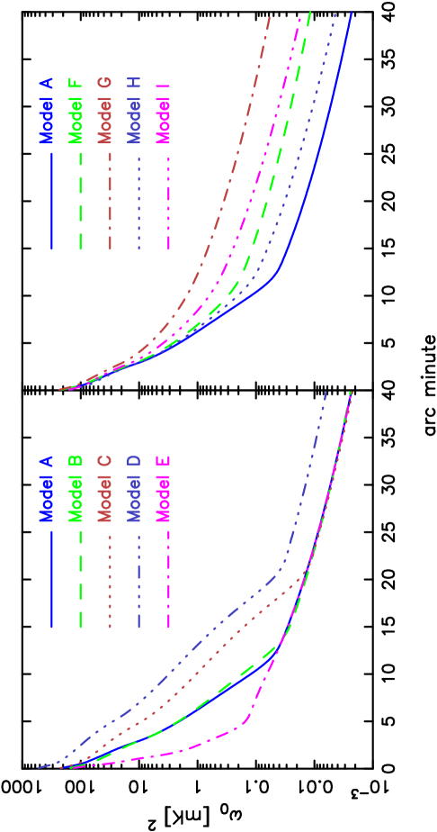
Figure 3: For the different models shown in Table 1, this shows the monopole of the signal expected at the epoch of reionization. Here $1^{{}^{\prime}}$ corresponds to $1.9h^{-1}{\rm Mpc}$ in the LCDM.

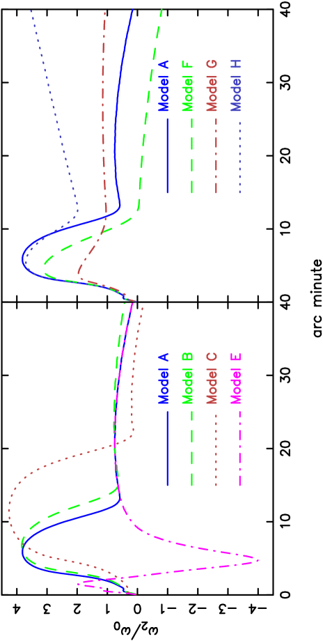
Figure 4: For the different models shown in Table 1, this shows the quadrupole to monopole ratio of the signal expected at the epoch of reionization. Here $1^{{}^{\prime}}$ corresponds to $1.9h^{-1}{\rm Mpc}$ in the LCDM.

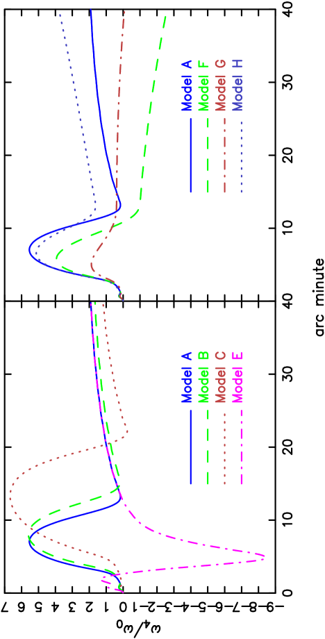
Figure 5: For the different models shown in Table 1, this shows the hexadecapole to monopole ratio of the signal expected at the epoch of reionization. Here $1^{{}^{\prime}}$ corresponds to $1.9h^{-1}{\rm Mpc}$ in the LCDM.

Considering next the anisotropy (Figure 4 and 5) we find that the dominant feature is a bump at small scales caused by the Poisson fluctuations from the discrete ionized bubbles. The location of the bump is sensitive to the size of the bubbles. The nature of the anisotropy is significantly altered if the Poisson fluctuations are not taken into account. The bump in the anisotropy is a consequence of the AP effect, as can be inferred from the fact that it is not changed much if the peculiar velocities are not taken into account. Further, this feature is not very sensitive to the background cosmological model. The bias $b_{c}$ of the ionized bubbles changes the amplitude of the bump. The large scale anisotropy is a combination of both the peculiar velocities and the AP effect which make opposite contributions to the anisotropy. The large scale anisotropy is nearly constant at a value which depends on both $b_{c}$ and $R$. Finally we note the fact that the signal is highly anisotropic with $w_{4}/w_{0}>w_{2}/w_{0}>1$, and it is possible that some of the higher angular moments not considered here have large values compared to $w_{0}$.

4.2 Post-reionization

We restrict our analysis here to $z=3.37$ which corresponds to frequency $325\,{\rm MHz}$ for the HI radiation. In addition to the possibility of different background cosmological models, there is only one free parameter $b$ namely the bias of the HI relative to the dark matter. We consider the LCDM model with $b=1$ as the fiducial model (Model J) for which Figures 6, 7 and 8 shows $w_{0}$, $w_{2}/w_{0}$ and $w_{4}/w_{0}$ respectively. The other models which we have considered are listed in Table 2.

The monopole $w_{0}$ (Figure 6) traces the dark matter distribution. Though the amplitude varies in the different models not much significance can be attached to this as such an effect can also arise from variations in the neutral fraction which is quite uncertain. The anisotropy in the clustering pattern is a combination of the peculiar velocities and the AP effect. This is deduced from the large change in the anisotropy when the peculiar velocity contribution is dropped. Both the effects are sensitive to the the background cosmological model at this redshift (Figures 1 and 2). The point to note is that changing the bias $b$ has an effect which is very similar to that of changing the background cosmological model, and it will be hard to use observations of the anisotropies to individually constrain any one of them.

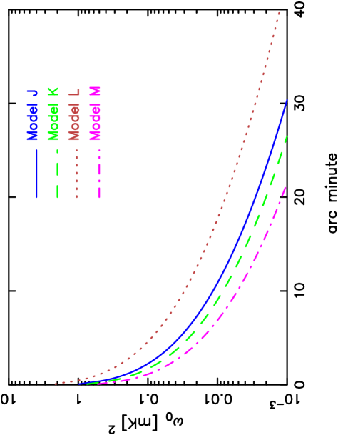
Figure 6: For the different models shown in Table 2, This shows the monopole for signal expected at $325\,{\rm MHz}$. Here $1^{{}^{\prime}}$ corresponds to $1.4h^{-1}{\rm Mpc}$ in the LCDM.

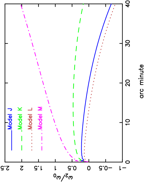
Figure 7: For the different models shown in Table 2, this shows the quadrupole to monopole ratio of the signal expected at $325\,{\rm MHz}$. Here $1^{{}^{\prime}}$ corresponds to $1.4h^{-1}{\rm Mpc}$ in the LCDM.

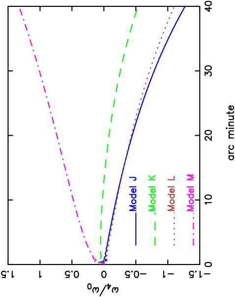
Figure 8: For the different models shown in Table 2, this shows the hexadecapole to monopole ratio of the signal expected at $325\,{\rm MHz}$ . Here $1^{{}^{\prime}}$ corresponds to $1.4h^{-1}{\rm Mpc}$ in the LCDM.

Table 2: This shows the different combinations for which we have calculated the signal expected at post-reionization. Here ${\rm b}$ is bias. Further, $\rm P.V$ indicates the peculiar velocities of HI.

Model	Background cosmology	$b$	$\rm P.V$
$\rm J$	$\rm LCDM$	1	$\surd$
$\rm K$	$\rm LCDM$	1.8	$\surd$
$\rm L$	$\rm VDE$	1	$\surd$
$\rm M$	$\rm LCDM$	1	$\times$

5 Discussion and conclusions.

The AP effect and the peculiar velocities both introduce anisotropies in the redshift space HI clustering pattern. These two sources of anisotropy are parameterized by two different functions $p(z)$ (Figure 1) and $f(z)$ (Figure 2) respectively, both of which depend on the background cosmological model. We have focused on two different background models. One of which has $\Omega_{m0}=0.3$ and $\Omega_{\Lambda 0}=0.7$ and another VDE model has $\Omega_{m0}=0.4$ and $\Omega_{\Lambda 0}=0.6$. The two models differ in that in one of the models the dark energy density remains a constant (LCDM) whereas in the other model (VDE) it increases with redshift and saturates at a value thrice the present value at $z\sim 3$. We find that $f(z)$ varies with the cosmological model only at low redshifts and it saturates at $f(z)=1$ at high redshifts where the universe is dark matter dominated in most cosmological models. Thus the anisotropies introduced by the peculiar velocities will be sensitive to the background cosmological model only at low redshifts, and it cannot tell us much about the background cosmological model at high redshifts. The function $p(z)$ is sensitive to the background cosmological models at nearly all redshifts $z>0.1$, and the anisotropies introduced by the AP effect hold the possibility of allowing us to probe the background cosmology at high redshifts.

We have considered simple models for the HI distribution at the epoch of reionization and in the post-reionization era. These models have a few parameters which quantify our ignorance about the HI distribution during these epochs. For the reionization era we have assumed that the total hydrogen content traces the dark matter, and the reionization proceeds through spherical bubbles of ionized gas of comoving radius $R$. Further, the centers of these bubbles could be biased with respect to the underlying dark matter. The HI in the post reionization era is assumed to be in high column density clouds which could be biased with respect to the underlying dark matter. For both the epochs we find that the anisotropies in the HI clustering pattern are sensitive to both, the background cosmological model and the free parameters determining the HI distribution. Given the fact that very little is known a-priori about the high redshift HI distribution, we conclude that it will not be possible to use observations of the anisotropies alone to uniquely constrain the background cosmological model. It may be noted that our findings contradict earlier claims (Nusser, 2004) where it was proposed that the anisotropies in the epoch of reionization HI signal could be used to constrain the background cosmological model.

We find that the anisotropy in the HI clustering is a combination of the contributions from both the AP effect and the peculiar velocities, and it cannot be attributed to anyone of them alone. Further, the anisotropy pattern at the epoch of reionization is very sensitive to the reionization model. In our simple model where the ionized bubbles are all of the same radius, we find a bump in the anisotropy pattern at the scales corresponding to the size of the bubbles. The bump will possibly be smeared in a more realistic situation where the bubbles will have a spread of sizes, but we may still expect a prominent feature at the scale corresponding to the characteristic bubble size. The anisotropy at large angular scales, we find, is sensitive to the bias of the centers of the ionized bubbles. Our analysis leads us to the conclusion that observations of the anisotropy in the HI clustering at the epoch of reionization will be a very powerful probe of the size, shape and distribution of the ionized regions the uncertainties in these being much more than the uncertainties in the background cosmological model. In the post-reionization era, the changes in the value of the bias parameter have a similar effect as changing the background cosmological model. These observations can be used to constrain the cosmological model if the bias parameter can be determined by independent means like the bi-spectrum (Verde et al. 1998; Scoccimarro 2000).

Finally we note that the temperature two-point correlation function considered here may not be the optimal statistical tool for detecting and quantifying the high redshift HI signal. The angular power spectrum (Zaldarriaga , Furlanetto & Hernquist, 2004) and the visibility correlations (Bharadwaj & Sethi 2001, Morales & Hewitt 2004 and Bharadwaj & Ali 2004b) have been proposed as optimal statistics for this purpose. In this paper we have chosen to study the temperature two-point correlation because of its similarity to the galaxy two-point correlation function where the anisotropy introduced by redshift space distortions is well understood and has received much attention in the literature. Though both the AP effect and the peculiar velocities are both included in Bharadwaj & Sethi (2001) and Bharadwaj & Ali (2004b), how to make the best use of these observations to constrain background cosmological models and models for the HI distribution still remains an open issue.

References

- Alam et al. (2004) Alam,U. , Sahni,V. ,Starobinsky, A. A. , 2004 ,JCAP ,0406 ,008
- Alcock & Paczynski (1979) Alcock , C. & Paczynski , B. , 1979 , Nature , 281 , 358
- Ballinger , Peacock , & Heavens (1996) Ballinger , W. E. , Peacock , J. A. , & Heavens , A. F. 1996 , MNRAS, 282 , 877
- Barkana & Loeb (2004a) Barkana R. & Loeb A. ,2004a ,ApJ, 624, L65
- Barkana & Loeb (2004b) Barkana R. & Loeb A. ,2004b ,ApJ, accepted , astro-ph/0410129
- Bharadwaj , Nath & Sethi (2001) Bharadwaj S. , Nath B. & Sethi S.K. ,2001 , JApA.22 ,21
- Bharadwaj & Sethi (2001) Bharadwaj , S. & Sethi , S. K., 2001 , JApA , 22 , 293
- Bharadwaj & Srikant (2004) Bharadwaj , S. & Srikant p ,s. 2004 , JApA , 25, 67
- Bharadwaj & Ali (2004a) Bharadwaj S. & Ali S. S., 2004a , MNRAS, 352, 142
- Bharadwaj & Ali (2004b) Bharadwaj S. & Ali S. S. ,2004b , MNRAS, 356, 1519
- Carroll (2001) Carroll ,S. M., 2001, Living Rev. Rel. 4,1
- Chen & Miralda-Escude (2004) Chen , X. & Miralda-Escude ,J. ,2004 , Ap.J, 602 , 1
- Ciardi et al. (2003) Ciardi , B. , Stoehr , & White , S.D.M. , 2003 , MNRAS , 343 , 1101
- Dekel & Lahav (1999) Dekel, A. , & Lahav,O. , 1999 , Ap.J, 520 , 24
- Field (1958) Field, G. B. ,1958, Proc. IRE , 46 , 240
- Furlanetto , Zaldarriaga & Hernquist (2004a) Furlanetto , S. R. , Zaldarriaga , M. & Hcernquist L. 2004a, Ap.J, 613, 1
- Furlanetto , Zaldarriaga & Hernquist (2004b) Furlanetto , S. R. , Zaldarriaga , M. & Hcernquist, L., 2004b , Ap.J, 613, 16
- Gnedin (2000) Gnedin , N. Y, 2000 ,Ap.J,535 , 530
- Hamilton (1992) Hamilton A. J. S. 1992 , Ap.J, 385 , L5
- Hawkins et al. (2002) Hawkins et al. 2002 , MNRAS, 346 , 78
- Hogan & Rees (1979) Hogan , C. J. & Rees , M. J. , 1979 , MNRAS ,188 ,791
- Hui & Haiman (2003) Hui , L. , & Haiman , Z. , 2003 , ApJ ,596 ,9
- Huterer & Turner (2001) Huterer, D & Turner, M.S , 2001 , Phys. Rev. D , 64 , 123527
- Kaiser (1987) Kaiser N., 1987 , MNRAS,227 ,1
- Kaiser (1984) Kaiser N., 1984 , ApJL ,284 ,L9
- Lanzetta , Wolfe & syosiTurnshek (1998) Lanzetta , K. M. , Wolfe , A. M. , Turnshek , D. A., 1995 , ApJ , 430 , 435
- Linder (2003) Linder, E. V., 2003, Phys. Rev. Lett., 90, 091301
- Loeb & Zaldarriaga (2004) Loeb A. & Zaldarriaga , M. ,2004, Phys. Rev. Lett., 92, 211301
- Matsubara & Suto (1996) Matsubara , T. & Suto , Y. ,1996 , apjl , 470 , L1
- Matsubara & Szalay (2002) Matsubara , T. & Szalay, A. S. ,2002 , Ap.J, 574 , 1
- Miralda-Escude (2003) Miralda-Escude ,J. ,2003 ,Science 300 ,1904-1909
- Morales & Hewitt (2004) Morales , M. F. and Hewitt , J. , 2004 , Ap.J, 615, 7
- Mo & White (1996) Mo, H.J. & , White, S.D.M. , 1996 , MNRAS, 282,347
- Nair (1999) Nair, V., 1999, Ap.J, 522, 569
- Nakamura , Matsubara , & Suto (1998) Nakamura , T. T. , Matsubara , T. , & Suto , Y. 1998 , Ap.J, 494 , 13
- Nusser (2004) Nusser, A. , 2004, preprint , astro-ph/0410420
- Peebles (1993) Peebles, P.J.E., Princpiles of Physical Cosmology, (Princeton Univ. Press: Princeton), 1993, pp 110
- Peebles & Ratra (1988) Peebles P. J. E.; & Ratra, B., 1988, ApJ, 325L, 17
- Perlmutter et al. (1999) Perlmutter S., et al. 1999, ApJ, 517, 565
- Perlmutter (2003) Perlmutter S., 2003, Physics Today, 56, 53
- Péroux et al. (2001) Péroux , C. , McMahon , R. G. , Storrie-Lombardi , L. J. & Irwin , M .J. 2003 , MNRAS , 346 , 1103
- Popowski et al. (1998) Popowski , P. A. , Weinberg , D. H. , Ryden , B. S. , & Osmer , P. S. 1998 , Ap.J, 498 , 11
- Ricotti & Ostriker (2004) Ricotti, M. & Ostriker, J. P., 2004, MNRAS, 352, 547
- Riess et al. (1998) Riess, A.G., et al 1998, AJ, 116, 1009
- Sahni & Starobinsky (2000) Sahni V. & Starobinsky A., 2000, Int. J. Mod. Phys. D, 9, 373
- Sahni & Wang (2000) Sahni V. & Wang L., 2000, Phys. Rev. D, 62, 103517
- Saini et al. (2000) Saini T., Raychaudhury S., Sahni V. & Starobinsky A.A., 2000, Phys. Rev. Lett., 85, 1162
- Scoccimarro (2000) Scoccimarro, R. 2000, Ap.J,544,597
- Scott & Rees (1990) Scott D. & Rees , M. J. , 1990 , MNRAS,247 ,510
- Sokasian et al. (2003a) Sokasian , A. Abel , T. Hernquist , L. & Springel , V. , 2003a , MNRAS , 344 , 607
- Sokasian et al. (2003b) Sokasian , A. , Yoshida , N. , Abel , T. , Hernquist , L. & Springel , V.S , 2003b , 350 , 47
- (52) Storrie–Lombardi , L. J. , McMahon , R. G. , Irwin , M. J., 1996 , MNRAS , 283 , L79
- (53) Swarup ,G , Ananthakrishnan ,S , Kapahi , V. K. , Rao , A. P., Subrahmanya , C. R.,Kulkarni , V. K. , 1991 , Curr. Sci. , 60 , 95
- Taruya & Suto (2001) Taruya, A. & Suto, Y. 2001, Ap.J,542,559
- Verde et al. (1998) Verde, L., Heavans, A.F., Matarrese, S. & Moscardini, L. 1998, MNRAS,300,747
- Wang & Tegmark (2004) Wang, Y. & Tegmark, M., 2004, Phys. Rev. Lett., 92, 241302
- Wouthuysen (1952) Wouthuysen, S. A. 1952, AJ, 57, 31
- Yoshikawa et al. (2001) Yoshikawa, K., Taruya , A. , Jing, Y.P. & Suto, Y. , 2001, ApJ, 558, 520
- Zaldarriaga , Furlanetto & Hernquist (2004) Zaldarriaga M. , Furlanetto , S. R. & Hernquits L. , 2004, ApJ, 608, 622