Cross correlations of X-ray and optically selected clusters with near infrared and optical galaxies

Abstract

We compute the real-space cluster-galaxy cross-correlation $\xi_{cg}(r)$ using the ROSAT-ESO Flux Limited X-ray (REFLEX) cluster survey, a group catalogue constructed from the final version of the 2dFGRS, and galaxies extracted from 2MASS and APM surveys. This first detailed calculation of the cross-correlation for X-ray clusters and groups, is consistent with previous works and shows that $\xi_{cg}(r)$ can not be described by a single power law. We analyse the clustering dependence on the cluster X-ray luminosity $L_{X}$ and virial mass $M_{vir}$ thresholds as well as on the galaxy limiting magnitude. We also make a comparison of our results with those obtained for the halo-mass cross-correlation function in a $\Lambda$CDM N-body simulation to infer the scale dependence of galaxy bias around clusters. Our results indicate that the distribution of galaxies shows a significant anti-bias at highly non-linear small cluster-centric distances ($b_{cg}(r)\simeq 0.7$), irrespective of the group/cluster virial mass or X-ray luminosity and galaxy characteristics, which show that a generic process controls the efficiency of galaxy formation and evolution in high density regions. On larger scales $b_{cg}(r)$ rises to a nearly constant value of order unity, the transition occuring at approximately $2\;h^{-1}$Mpc for 2dF groups and $5\;h^{-1}$Mpc for REFLEX clusters.

1 Introduction

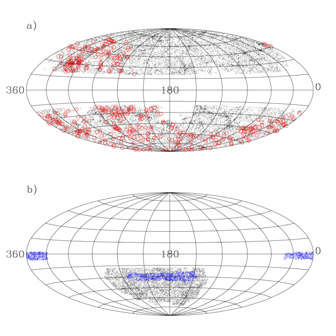
Figure 1: a) Aitoff projection of the distribution, in galactic coordinates, of 2MASS galaxies with $K_{s}<12.5$ (dots) together with the REFLEX cluster sample (red circles). The angular mask described in section 2.2 has been applied to both samples. b) Aitoff projection of the distribution, in equatorial coordinates, of 10% of APM galaxies with $b_{j}<18.5$ (black dots) and all 2dFGGC (blue dots).

Statistical analysis of clusters and groups of galaxies are among the most powerful tools for the study of large scale structure. In the hierarchical clustering scenario, these objects form by the gravitational amplification of primordial density fluctuations, so that they can be used to characterize the spatial distribution of the peaks of the density field. Besides, as they are the largest gravitationally bound objects and span a wide range of masses, they can be used as laboratories to determine the role of the different astrophysical processes that govern galaxy formation.

The first statistical analysis on this type of objects where based on cluster catalogues constructed by visual identification (Abell, 1958; Abell, Olowin & Corwin, 1989). The cluster-cluster correlation function $\xi_{cc}(r)$ has been the preferred tool for such analysis, providing a simple and convenient statistical tool to characterize their spatial distribution and place constraints on cosmological models (Bahcall & Soneira 1983; Klypin & Kopylov 1983; Peacock & West 1992; Postman, Huchra & Geller 1992). Nonetheless, clear evidence of inhomogeneities and line-of-sight projection effects was found (Lucey 1983; Sutherland 1988), which where responsible for part of the observed amplitude of the angular correlation. The situation improved with digitized cluster surveys like the Edinburgh/Durham Cluster Catalogue (Nichol et al. 1992) and the APM survey (Dalton et al 1992, 1994; Croft et al 1997). Although these where more homogeneous, systematics due to projection effects are inherent to cluster identification based on angular positions in the sky (Padilla & Lambas, 2003).

In recent years, X-ray information has been used to construct new cluster samples. This method of identification has several advantages with respect to the use of optical data. The X-ray emission is a strong signature of a gravitational potential well since there is a strong relation between the X-ray luminosity $L_{X}$ and mass (Reiprich & Böhringer 2002). Besides the emissivity of thermal Bremsstrahlung radiation is proportional to the square of the electron density thus it provides clear evidence of a mass concentration which is not strongly affected by projection effects. Furthermore, the X-ray emission from the clusters is concentrated towards the dense central core giving an improved angular resolution compared to the one obtained using galaxy concentrations, also helping to reduce the possibility of projection effects. The ROSAT-ESO Flux Limited X-ray (REFLEX) cluster survey (Böhringer et al. 2004), comprising 447 objects, is the largest statistically complete X-ray selected sample. It has been previously used to analyse the large scale structure through its power spectrum (Schuecker et al. 2001) and its correlation function (Collins et al., 2000). Although Schuecker et al. (2001) found a systematic increase of the amplitude of the power spectrum with limiting X-ray luminosity, Collins et al. (2001) results lack such a trend in the correlation function, characterized by an approximate power-law with correlation length $r_{0}=18.8\pm 0.9\;h^{-1}\rm{Mpc}$.

On the other hand, since the advent of large galaxy redshift surveys a reliable identification of groups of galaxies has been possible using not only angular positions, but also the complete redshift information, avoiding in this way a strong contamination by projection effects. The first algorithms designed for this task where developed by Huchra & Geller (1982) and Nolthenius & White (1987). These methods where based on the friends-of-friends algorithm used in numerical simulations with a redshift dependent linking length parameter. A variety of group catalogues where constructed using this algorithms: Merchán et al. (2000) used the Updated Zwicky Catalogue (Falco et al. 1999), Giuricin et al. (2000) constructed a group catalogue from the Nearby Optical Galaxy Sample, Tucker et al. (2000) extracted a group sample from the Las Campanas Redshift Survey (Shectman et al. 1996), and Ramella et al. (2002) used the information of the Updated Zwicky catalogue and the Southern Sky Redshift Survey (da Costa et al. 1998). Recently, the 100K public data release of the 2dF Galaxy Redshift Survey (2dFGRS, Colles et al. 2001) has been used by Merchán & Zandivarez (2002) to construct one of the largest group catalogues using a slight modification of the Huchra & Geller (1982) algorithm. The large scale redshift space distribution of this sample has been studied by Zandivarez, Merchán & Padilla (2003). They showed that the redshift space correlation function has a power law behavior with a correlation length of $s_{0}=8.9\pm 0.3\;h^{-1}\rm{Mpc}$.

The cluster and group catalogues identified by X-ray information or three dimensional percolation algorithms, represent different types of objects. In order to be able to confront the results obtained for these samples with the predictions of theoretical models, a complete understanding of the differences in the statistical properties of the samples is crucial. One of the most important possible comparisons is the analysis of the clustering of galaxies, selected in different wave-bands, around these objects and how it depends on the properties like X-ray luminosity or virial mass. The best statistical tool for such analysis is the two-point cluster-galaxy cross-correlation function $\xi_{cg}(r)$, which is a measure of the mean radial density profile around clusters. The first measurement of this correlation function was performed by Seldner & Peebles (1977), who studied the angular cross-correlation of Abell clusters and Lick galaxies. They found that $\xi_{cg}(r)$ was very large and positive out to scales as large as $r\simeq 100\;h^{-1}\rm{Mpc}$ but they where contradicted by Lilje & Efstathiou (1988) who did not find any strong evidence of clustering beyond $r>=20\;h^{-1}\rm{Mpc}$ arguing that part of the signal detected by Seldner & Peebles (1977) was a consequence of artificial surface density gradients in the Lick catalogue. At smaller scales, Lilje & Efstathiou (1988) found that $\xi_{cg}(r)$ was well fitted by a power law with $r_{0}=8.8\;h^{-1}\rm{Mpc}$. Later works (Dalton 1992; Mo, Peacock & Xia 1993; Moore et al. 1994) found similar results based on direct measurements from redshift surveys of galaxies and clusters. They found that $\xi_{cg}(r)$ has a similar shape to $\xi_{cc}(r)$ and $\xi_{gg}(r)$ but with an amplitude approximately equal to their geometric mean. Croft et al. (1999) estimated $\xi_{cg}(r)$ in real and redshift-space from the APM galaxy and cluster surveys and found that its shape can not be described by a single power law and that its amplitude is almost independent of cluster richness and the limiting magnitude of galaxies.

In this paper we compute $\xi_{cg}(r)$ using a sample of groups derived from the final version of the 2dFGRS and the REFLEX cluster survey, and the galaxies from the 2MASS (Skrutskie et al. 1997) and APM (Maddox et al. 1990) surveys. The outline of the paper is as follows, in section §2 we describe the different data sets analysed in this work. In §3 we describe the method used to obtain the 3D real space cluster-galaxy cross-correlation function from the projected cross-correlation function. In §4 we test the dependence of our results on the magnitude limit in the galaxy catalogue, the X-ray luminosity $L_{X}$ in the REFLEX catalogue and the virial mass $M_{vir}$ in the 2dF Galaxy Group Catalogue. In §5 we show a comparison with the results of an N-body simulation of the $\Lambda$CDM cosmological model. Finally, in §6 we present a short discussion and our main conclusions.

2 The Data

2.1 Galaxy catalogues

Figure 2: Redshift distribution of the different samples of clusters and galaxies analysed in this work. It can be seen that the distribution of the REFLEX clusters peaks at approximately the same redshift as 2MASS galaxies.

We used the information from the Two Micron All Sky Survey (2MASS; Skrutskie et al. 1997). 2MASS characterize the large scale distribution of galaxies in the near-infrared using the $K_{s}$ ($2.15\mu$m) passband. Our data set was selected from the public full-sky extended source catalogue (XSC; Jarret et al. 2000) which contains over 1.1 million extended objects brighter than $K_{s}=14$mag. The raw magnitudes where corrected for Galactic extinction using the IR reddening map of Schlegel, Finkbeiner & Davis (1998). There is a strong correlation between dust extinction and stellar density, which increases exponentially towards the galactic plane. Stellar density is a contaminant factor of the XSC since the reliability of separating stars from extended sources is very sensitive to this quantity (Jarret et al. 2000). In order to avoid contamination from stars we have constructed a mask for the 2MASS survey using a $HEALPIX$ (Gorski et al. 1999) map with $Nside=256$ and excluding those pixels where the $K_{s}$ band extinction $A(K_{s})=0.367\times E(B-V)>0.05$ and $\left|b\right|>20^{o}$ which reduces galactic contaminant sources to $2\%$ (Maller et al., 2003). We also followed Maller et al. (2003) and imposed a cut at $K_{s}=13.57$ mag in the corrected magnitudes. Figure 1 shows an Aitoff projection of the final sample obtained with these restrictions, which contains 397447 galaxies.

We also used information from the APM Galaxy Survey (Maddox et al. 1990), which is based on 185 UK IIIa-J Schmidt photographic plates each corresponding to a $5.8\times 5.8$ $deg^{2}$ on the sky limited to $b_{j}\simeq 20.5$ and with a mean depth of $\simeq 400\;h^{-1}\rm{Mpc}$ for $b<-40^{o}$ and $\delta<-20^{o}$. We selected our galaxy sample from the APM survey imposing the cut $b_{j}<20.5$. The sub-sample with $b_{j}<18.5$ is also shown in Figure 1.

Galaxy $K_{s}$ luminosity is less sensitive to dust and stellar populations than the $B$ band, providing a more uniform survey of the galaxy population. The $K_{s}$ band also gives a better measure of the stellar mass content than the $B$ band. Then, the variations of the correlation function of samples selected in these bands can give us valuable information on the dependence of galaxy bias on the various properties of galaxies and then shed some light in their formation and evolution.

2.2 Cluster and group catalogues

In our analysis we used information of the ROSAT-ESO X-ray Flux Limited (REFLEX) Cluster Survey (Böhringer et al., 2004). The geometry of the survey is described by the southern hemisphere with $\delta<+2.5^{o}$ excluding the zone where $\left|b\right|<20^{o}$ and the Small and the Large Magellanic Clouds, covering an area of 4.24sr. The sample has a nominal flux limit of $3\times 10^{-12}\rm{erg\,s^{-1}cm^{-2}}$ within the ROSAT energy band (0.1-2.4)keV and comprises 447 clusters. Figure 1 shows an Aitoff projection of the 422 clusters inside the 2MASS mask described in section 2.1.

We also used a group catalogue (hereafter the 2dF Galaxy Group Catalogue, 2dFGGC) constructed from the final version of the 2dF Galaxy Redshift Survey (2dFGRS, Colless et al. 2001), using the same technique used by Merchán & Zandivarez (2002) to construct the group catalogue of the 2dFGRS 100K release (Folkes et al. 1999). This sample comprises 5568 groups for which virial mass, velocity dispersion and virial radius have been determined.

These samples where determined using very different types of information. The strong relation between $L_{X}$ and $M$ (see e.g. Reiprich & Böhringer, 2002) indicates that X-ray selected clusters samples are close to be basically selected by mass. The situation is very different for optically selected groups and clusters where the selection criteria is based on richness, which is not a good mass indicator. The study of the differences in the way in which galaxies cluster around them can be very important to improve our knowledge of this type of objects and to understand their overall statistical properties.

Figure 2 shows the redshift distribution of the samples analysed in this work. The distribution for 2MASS galaxies was obtained by Maller et al. (2004) by matching it with SDSS Early Data Release (Stoughton et al. 2002) and the 2dFGRS 100K release (Colles et al. 2001). For APM galaxies we used the fit from Baugh & Efstathiou (1993). It can be seen that the distribution for the REFLEX cluster survey peaks at approximately the same redshift as 2MASS galaxies. As we measure the projected cross-correlation function (see section 3), the largest contribution to this function will come for cluster-galaxy pairs laying at similar redshifts, which enhances our signal, on the other hand the differences with the distribution of APM galaxies will cause a lower amplitude in the projected correlations.

3 Cluster-Galaxy Correlations

Figure 3: The upper panels show the projected cross-correlation function $\omega_{cg}(\sigma)$ obtained for REFLEX clusters and 2dF groups against APM (right) and 2MASS (left) galaxies for three different magnitude limits. In both cases the error bars where obtained by the bootstrap re-sampling technique. The lower panels show the correspondent 3D real-space cross-correlation function recovered from $\omega_{cg}(\sigma)$.

The spatial cluster-galaxy cross-correlation function $\xi_{cg}(r)$ is defined so that the probability $dP$ of finding a galaxy in the volume element $dV$ at a distance $r$ from the center of a cluster is

$$dP=\bar{n}\left[1+\xi_{cg}(r)\right]dV,$$ (1)

where $\bar{n}$ is the mean space density of galaxies. We only have information on the distance (redshifts) of the clusters and not on the individual galaxies in the 2MASS and APM catalogues. Then, in order to obtain $\xi_{cg}(r)$ we first determine the projected cross-correlation function $\omega_{cg}(\sigma)$, defined by Lilje & Efstathiou (1988), where $\sigma=cz\theta/H_{0}$ is the projected separation between a cluster at redshift $z$ and a galaxy at angular distance $\theta$ from its centre. To determine this quantity from our data we used the estimator

$$\omega(\sigma)=\frac{\left\langle CG(\sigma)\right\rangle}{\left\langle CR(\sigma)\right\rangle}\frac{N_{R}}{N_{G}}-1,$$ (2)

where $N_{G}$ is the number of galaxies, $\left\langle CG(\sigma)\right\rangle$ is number of cluster-galaxy pairs at a projected distance $\sigma$, and $\left\langle CR(\sigma)\right\rangle$ is the analogous quantity defined for a random distribution of $N_{R}$ points covering the same angular mask than the original galaxy survey.

When the angle $\theta\ll 1$ rad, that is, the distance $y$ to the cluster centre is much larger than the projected cluster-galaxy separation, the projected correlation function is related to the spatial correlation function by the simple integral equation (Saunders, Rowan-Robinson & Lawrence, 1992)

$$\xi(r)=-\frac{1}{B\pi}\int_{r}^{\infty}\frac{d\omega_{cg}(\sigma)}{d\sigma}\frac{1}{(\sigma^{2}-r^{2})^{1/2}}d\sigma.$$ (3)

The constant $B$ regulates the amplitude of the correlation function taking into account the differences in the selection function of clusters and galaxies and can be calculated by (Lylje & Efstathiou 1988)

$$B=\frac{\sum_{i}\psi(y_{i})}{\sum_{i}\frac{1}{y_{i}^{2}}\int_{0}^{\infty}\psi(x)x^{2}dx},$$ (4)

where $\psi(y)$ is the selection function of the galaxy survey, $y_{i}$ is the distance to cluster $i$ and the sums extends to all clusters in the sample.

Equation 3 can be easily solved analytically if we perform a linear interpolation of $\omega_{cg}$ between its values at the measured $\sigma$’s. With this approach the solution to equation 3 is (Saunders, Rowan-Robinson & Lawrence, 1992)

$$\xi_{cg}(\sigma_{i})=-\frac{1}{B\pi}\sum_{i\leq j}\frac{\omega_{j+1}-\omega_{j}}{\sigma_{j+1}-\sigma_{j}}\ln\left(\frac{\sigma_{j+1}+\sqrt{\sigma_{j+1}^{2}-\sigma_{i}^{2}}}{\sigma_{j}+\sqrt{\sigma_{j}^{2}-\sigma_{i}^{2}}}\right).$$ (5)

We used this expression to obtain $\xi_{cg}$ from $\omega_{cg}$. In order to calculate the factor $B$ we evaluated the selection function $\psi(y)$ by

$$\psi(y)=\int_{L_{min}(y)}^{\infty}\phi(L)\,\rm{dL},$$ (6)

where $L_{min}(y)$ is the minimum luminosity that a galaxy at distance $y$ must have in order to be included in the catalogue and $\phi(x)$ is the luminosity function, for which we used the parameters of Bell et al. (2003) for 2MASS and Loveday et al. (1992) for APM.

4 RESULTS

4.1 The projected and 3D real-space cross-correlation function

The upper panels of Figure 3 show the projected cross-correlation function $\omega_{cg}(\sigma)$ obtained for REFLEX clusters and 2dF groups against APM (right) and 2MASS (left) galaxies for three different magnitude limits. In both cases the error bars where obtained by the bootstrap re-sampling technique. Specially for 2dF groups, the shape of this function is different from a simple power law as it shows an increment in small scales that can be associated to the inner profile of the groups and clusters.

Table 1: Results for power-law fits of the form $\xi_{cg}(r)=(r/r_{0})^{\gamma}$ to the inner and outer regions of $\xi_{cg}(r)$ for the different samples analysed using the REFLEX clusters as centres.

REFLEX sample	Galaxy sample	$r^{inner}_{0}$	$\gamma^{inner}$	$r^{outer}_{0}$	$\gamma^{outer}$
all	2MASS $K_{s}<12.5$	$6.1^{+1.1}_{-0.6}$	$-2.60^{+0.26}_{-0.17}$	$10.3^{+0.90}_{-1.17}$	$-1.55^{+0.17}_{-0.19}$
all	2MASS $K_{s}<13.0$	$6.2^{+1.1}_{-0.7}$	$-2.52^{+0.22}_{-0.19}$	$9.85^{+0.67}_{-0.73}$	$-1.69^{+0.09}_{-0.14}$
all	2MASS $K_{s}<13.57$	$5.97^{+1.30}_{-0.46}$	$-2.62^{+0.19}_{-0.15}$	$9.18^{+0.60}_{-0.59}$	$-1.77^{+0.13}_{-0.12}$
all	APM $b_{j}<18.5$	$5.47^{+0.64}_{-0.38}$	$-2.69^{+0.24}_{-0.10}$	$9.9^{+1.0}_{-1.1}$	$-1.67^{+0.16}_{-0.15}$
all	APM $b_{j}<19.5$	$5.47^{+1.0}_{-0.4}$	$-2.61^{+0.25}_{-0.17}$	$10.4^{+1.3}_{-1.1}$	$-1.71^{+0.13}_{-0.14}$
all	APM $b_{j}<20.5$	$5.54^{+0.88}_{-0.38}$	$-2.65^{+0.21}_{-0.14}$	$9.5^{+1.2}_{-1.0}$	$-1.79^{+0.16}_{-0.19}$
$\log(L_{X}/10^{44}\rm{erg\ s^{-1}})>-1.5$	2MASS $K_{s}<13.57$	$5.96^{+0.79}_{-0.46}$	$-2.62^{+0.19}_{-0.15}$	$9.18^{+0.59}_{-0.59}$	$-1.77^{+0.13}_{0.13}$
$\log(L_{X}/10^{44}\rm{erg\ s^{-1}})>-1.0$	2MASS $K_{s}<13.57$	$6.24^{+0.95}_{-0.61}$	$-2.57^{+0.18}_{-0.18}$	$10.28^{+0.67}_{-0.66}$	$-1.70^{+0.14}_{-0.13}$
$\log(L_{X}/10^{44}\rm{erg\ s^{-1}})>-0.85$	2MASS $K_{s}<13.57$	$6.24^{+0.83}_{-0.57}$	$-2.58^{+0.21}_{-0.22}$	$10.45^{+0.58}_{-0.65}$	$-1.75^{+0.10}_{-0.12}$
$\log(L_{X}/10^{44}\rm{erg\ s^{-1}})>-0.5$	2MASS $K_{s}<13.57$	$6.41^{+0.45}_{-0.27}$	$-2.75^{+0.11}_{-0.06}$	$10.8^{+1.2}_{-0.7}$	$-1.75^{+0.11}_{-0.12}$
$\log(L_{X}/10^{44}\rm{erg\ s^{-1}})>0$	2MASS $K_{s}<13.57$	$7.13^{+0.89}_{-0.44}$	$-2.72^{+0.27}_{-0.07}$	$13.1^{+1.1}_{-1.1}$	$-1.69^{+0.15}_{-0.18}$

Table 2: Results for power-law fits of the form $\xi_{cg}(r)=(r/r_{0})^{\gamma}$ to the inner and outer regions of $\xi_{cg}(r)$ for the different samples analysed using 2dF groups as centres.

2dF Groups sample	Galaxy sample	$r^{inner}_{0}$	$\gamma^{inner}$	$r^{outer}_{0}$	$\gamma^{outer}$
all	2MASS $K_{s}<12.5$	$1.9^{+1.6}_{-0.5}$	$-3.28^{+0.32}_{-0.26}$	$6.28^{+0.20}_{-0.22}$	$-1.60^{+0.07}_{-0.07}$
all	2MASS $K_{s}<13.0$	$2.2^{+1.5}_{-0.6}$	$-2.78^{+0.34}_{-0.35}$	$6.21^{+0.21}_{-0.21}$	$-1.51^{+0.06}_{-0.06}$
all	2MASS $K_{s}<13.57$	$2.1^{+1.2}_{-0.3}$	$-2.90^{+0.25}_{-0.40}$	$5.18^{+0.18}_{-0.20}$	$-1.58^{+0.06}_{-0.06}$
all	APM $b_{j}<18.5$	$1.8^{+1.1}_{-0.2}$	$-1.75^{+0.50}_{-0.61}$	$6.65^{+0.33}_{-0.37}$	$-1.37^{+0.08}_{-0.08}$
all	APM $b_{j}<19.5$	$2.6^{+1.3}_{-0.7}$	$-2.02^{+0.59}_{-0.69}$	$5.71^{+0.35}_{-0.35}$	$-1.42^{+0.09}_{-0.09}$
all	APM $b_{j}<20.5$	$2.5^{+1.1}_{-0.6}$	$-2.20^{+0.43}_{-0.61}$	$4.82^{+0.34}_{-0.36}$	$-1.46^{+0.12}_{-0.11}$
$\log(M_{vir}/M_{\odot})>13$	2MASS $K_{s}<13.57$	$1.95^{+0.53}_{-0.16}$	$-3.23^{+0.82}_{-0.55}$	$6.73^{+0.27}_{-0.25}$	$-1.52^{+0.06}_{0.07}$
$\log(M_{vir}/M_{\odot})>13.5$	2MASS $K_{s}<13.57$	$2.29^{+0.65}_{-0.13}$	$-3.47^{+0.94}_{-0.31}$	$8.21^{+0.39}_{-0.35}$	$-1.59^{+0.08}_{-0.07}$
$\log(M_{vir}/M_{\odot})>14$	2MASS $K_{s}<13.57$	$5.7^{+1.2}_{-1.1}$	$-2.47^{+0.29}_{-0.28}$	$10.6^{+1.0}_{-1.1}$	$-1.63^{+0.15}_{-0.17}$
$\log(M_{vir}/M_{\odot})>14.5$	2MASS $K_{s}<13.57$	$6.3^{+1.5}_{-1.5}$	$-2.74^{+0.47}_{-0.42}$	$10.8^{+1.7}_{-1.5}$	$-1.84^{+0.35}_{-0.35}$

The lower panels of Figure 3 show the corresponding 3D real-space cross-correlation function recovered from $\omega_{cg}(\sigma)$. Our findings are in complete agreement with the results of Croft et al. (1999, see their figure 2). We found that the shape of the correlation function can not be described as a single power law for all scales, as it becomes steeper at small scales. Tables 1 and 2 show the results of power-law fits of the form $\xi(r)_{cg}=(r/r_{0})^{\gamma}$ to the inner and outer regions for the different samples analysed. It can be clearly seen that the correlation function is nearly independent of the magnitude limit imposed to the galaxy sample showing only small variations in the best fit power-law parameters. The shape of the cross-correlations obtained for 2MASS and APM galaxies are different. The feature at $r\simeq 2\;h^{-1}\rm{Mpc}$ that show the transition to the inner profile of the clusters is more evident for 2MASS galaxies. This effect can be associated with differences in the spatial distribution of these objects around clusters. 2MASS galaxies where selected in the near-infrared and so would tend to be luminous and of early type morphologies, and so, are expected to have a stronger clustering (Norberg et al. 2002).

4.2 Dependence on $L_{X}$ and $M_{vir}$

In order to analyse the dependence of the distribution of galaxies around clusters and groups on properties such as their mass or X-ray luminosity we have computed $\xi_{cg}(r)$ for 2MASS galaxies and the REFLEX cluster survey for four different limits on $L_{X}$. Analogously for 2dFGGC we have adopted four different limits in $M_{vir}$. The results obtained for these samples are shown in figures 4 and 5. We find a clear dependence of the amplitude of $\xi_{cg}(r)$ on $L_{X}$ which indicates that galaxies are more clustered around more luminous (massive) objects. The value of the amplitude of the correlaction function for the outer region changes from $r_{0}=9.18\pm 0.59$ for $\log(L_{X}/10^{44}\rm{erg\ s^{-1}})>-1.5$ to $r_{0}=13.1\pm 1.1$ for $\log(L_{X}/10^{44}\rm{erg\ s^{-1}})>0$ and the inner region shows a similar behaviour. The shape of $\xi_{cg}(r)$ does not show any important differences, but the small changes of $\gamma^{inner}$ show a weak indication that a higher limiting $L_{X}$ produce steeper inner regions.

The changes in $\xi_{cg}(r)$ for 2dF groups and 2MASS varying the limiting virial mass are even stronger. The overall shape of $\xi_{cg}(r)$ changes, specially for small scales where the amplitude increase from the sample with $\log(M_{vir}/M_{\odot})>13$ to the one with $\log(M_{vir}/M_{\odot})>14.5$ is a factor 20 whereas for scales $r\simeq 10\;h^{-1}\rm{Mpc}$ the increase is a factor 5. The value of $\gamma$ in the outer region also increase with $M_{vir}$ and for $\log(M_{vir}/M_{\odot})>14.5$ its value is simmilar to the one in the inner region.

Figure 4: The real space cluster-galaxy cross-correlation functions of REFLEX clusters and all 2MASS galaxies for different X-ray luminosity limits.

Figure 5: The real space cluster-galaxy cross-correlation functions of 2dFGGC and all 2MASS galaxies for different limits on $M_{vir}$. For comparison $\xi_{cg}(r)$ for REFLEX clusters with $\log(L_{X}/10^{44}\rm{erg\ s^{-1}})>-0.85$ and 2MASS galaxies is also shown.

Figure 5 also shows for comparison $\xi_{cg}(r)$ for REFLEX clusters with $\log(L_{X}/10^{44}\rm{erg\ s^{-1}})>-0.85$. Its similarity with the cross-correlation function obtained using 2dF groups with $\log(M_{vir}/M_{\odot})>14$ is remarkable. This fact can be used as an indirect test of the $L_{X}-M$ relation. Reiprich & Böhringer (2002) found a power law relation between $L_{X}$ in the ROSAT energy band (0.1-2.4 keV) and the mass $M_{200}$ (where $M_{200}=M_{total}(r<r_{200})$) of the form

$$\log\left[\frac{L_{X}}{h_{50}^{-2}10^{40}\rm{erg\ s^{-1}}}\right]=A+\alpha\log\left(\frac{M_{200}}{h_{50}^{-1}M_{\odot}}\right).$$ (7)

The transformation from $M_{vir}$ to $M_{200}$ can be done assuming a given density profile for the clusters (see White 2000). For a $\Lambda$CDM the difference is small ($M_{vir}\simeq 1.2M_{200}$). Then, assuming $h=0.7$, $A=-20.055$ and $\alpha=1.652$ (from table 7 in Reiprich and Böhringer, 2002), $\log(M_{vir}/h^{-1}M_{\odot})=14.0$ corresponds to $\log(L_{X}/10^{44}\rm{erg\ s^{-1}})=-0.85$ in excellent agreement with the limit imposed to the sample used in figure 5.

5 Comparison with the results of $\Lambda$CDM N-body simulations

Figure 6: The results for $b_{cg}(r)$ for all the samples analysed in this work obtained by the comparison with the results of a $\Lambda$CDM N-body simulation. Different lines show the results obtained for samples selected with different limiting mass given by $m_{1}=7.5\times 10^{13}\,M_{\odot}$ (dot-dashed), $m_{2}=1.4\times 10^{14}\,M_{\odot}$ (long dashed), $m_{3}=4.1\times 10^{14}\,M_{\odot}$ (short dashed) and $m_{4}=7.5\times 10^{14}\,M_{\odot}$ (solid).

In order to make a comparison between our results and those corresponding to the concordance cosmological model we used the $\Lambda$CDM Very Large Simulations (VLS). This simulations where carried out by the Virgo Supercomputing Consortium using computers based at Computing Centre of the Max-Planck Society in Garching and at the Edinburgh Parallel Computing Centre. The data are publicly available at www.mpa-garching.mpg.de/NumCos. It uses $512^{3}$ particles in a box of $480\;h^{-1}\rm{Mpc}$, with initial conditions consistent with a $\Lambda$CDM power spectrum computed using CMBFAST (Seljak & Zaldarriaga, 1996), normalized so that $\sigma_{8}=0.9$. We have identified groups using a Friends-Of-Friends (FOF) algorithm with a linking parameter $b=0.2$ and we used these halos as centres to measure the halo-mass cross-correlation function $\xi_{hm}(r)$ for different values of limiting mass. We used these results to infer the scale dependence of the cluster-galaxy bias factor, that is the bias between the distribution of galaxies and mass around clusters, defined by

$$b_{cg}(r)=\xi_{cg}(r)/\xi_{hm}(r).$$ (8)

For small scales this is simply the difference between the density profile of mass and galaxies.

In order to obtain $b_{cg}(r)$ we used four values of the limiting mass to measure $\xi_{hm}(r)$: $m_{1}=7.5\times 10^{13}\,M_{\odot}$, $m_{2}=1.4\times 10^{14}\,M_{\odot}$, $m_{3}=4.1\times 10^{14}\,M_{\odot}$ and $m_{4}=7.5\times 10^{14}\,M_{\odot}$. As the REFLEX clusters and the 2dF groups span different ranges of mass, we used the 2dFGGC as centres to calculate $\xi_{cg}(r)$ for $m_{1}$ and $m_{2}$, and the REFLEX catalogue for $m_{3}$ and $m_{4}$. When using the 2dFGGC we simply imposed the same limits in $m_{vir}$. For the REFLEX clusters, we used the X-ray luminosity threshold for which the abundance, calculated by the integration of the X-ray luminosity function of Böhringer et al. (2002), gives the same values as those obtained in the simulation. The results obtained are shown in Figure 6.

Our results for the two lower values of the threshold mass show that, at large scales, $b_{cg}(r)$ is consistent with a constant of order $b_{cg}\simeq 1$ for APM galaxies and slightly higher for 2MASS, which shows that 2MASS galaxies are more biased tracers of the mass distribution than optically selected galaxies. On smaller scales ($r<2\;h^{-1}\rm{Mpc}$) the distribution of galaxies around clusters shows a significant and nearly constant anti-bias of $b_{cg}\simeq 0.7$. For $m_{3}$ and $m_{4}$, $b_{cg}(r)$ shows the same behavior but with a larger transition scale between the two regimes ($r\simeq 2\;h^{-1}\rm{Mpc}$). In all cases this scale would correspond to the onset of non-linearities, where $\xi_{cg}(r)$ becomes steeper and virialization takes place. A constant bias is a feature characteristic of linear theory and then it is not surprising that it does not hold as well in the non-linear regime. Another reason that may add to the anti-bias in the cluster and infall regions is the change in the galaxy types. The dense environments contain galaxies with older stellar populations with less light per baryonic mass. Then, cluster regions are down-weighted by this effect. It is very important to note that these results are independent of the limiting values of mass, X-ray luminosity and magnitude used to construct the clusters and galaxy samples, which shows that this is not a property of a given galaxy type, but a generic feature of the processes that control the efficiency of galaxy formation and evolution.

6 Discussion and Conclusions

In this work we have performed the first detailed calculation of the 3D real-space cluster-galaxy cross-correlation for an X-ray selected cluster sample and galaxies selected in the optical and near-infrared wave-bands. We have also presented the first calculation of this statistical measure for a galaxy group sample from the 2dFGRS. These two samples span a wide range of masses and so they allow us to analyse the dependence of $\xi_{cg}(r)$ on $M_{vir}$. Our results for the different sub-samples of galaxies from 2MASS or APM with different limiting magnitudes show that $\xi_{cg}(r)$ is almost independent of galaxy properties and that its shape is determined almost exclusively by the criteria used to define the cluster sample.

In agreement with previous works (Croft et al. 1999) we found that the shape of $\xi_{cg}(r)$ can not be described by a single power law at all scales. Instead, it shows two regimes with a clear transition, one for the larger scales, and a steeper one at smaller scales showing the inner profiles of the distribution of galaxies around cluster centres. We have used our results to check the $L_{X}-M$ relation of Reiprich & Böhringer (2002). We have found that the correlation functions obtained using 2dF groups with a given lower mass limit and REFLEX clusters with the corresponding limit on $L_{X}$ are in complete agreement showing the validity of this relation.

The comparison of our results with those obtained for the halo-mass cross-correlation function in a $\Lambda$CDM N-body simulation shows that the observational results are consistent with a constant bias on large scales of order unity for APM galaxies and slightly higher for 2MASS galaxies. On smaller scales our results suggests that there is a substantial anti-bias ($b_{cg}(r)\simeq 0.7$). In all cases the transition scale between the two regimes corresponds to the onset of non-linearities, where the correlation functions becomes steeper. This is a strong result of our analysis which is independent of the properties of the cluster or galaxy samples used, showing that it is simply a generic feature of the different processes that govern galaxy formation and their subsequent evolution.

References

- [1] Abell G. O., 1958, ApJS, 3, 211
- [2] Abell G. O., Corwin H.G., Corwin H.G., 1989, ApJS, 70,1
- [3] Bahcall N.A., Soneira R.M., 1983, ApJ, 270, 20
- [4] Baugh C.M., and Efstathiou G., 1993, MNRAS, 265, 145
- [5] Bell E.F., McIntosh D.H., Katz N., and Weinberg M.D., 2003, ApJS, 149, 289
- [6] Böhringer H., Collins C.A., Guzzo L., Schuecker P., Voges W., Neumann D.M., Schindler S., Chincarini G., De Grandi S., Cruddace R.G., Edge A.C., Reiprich T.H., Shaver P.H., 2002, ApJ, 566, 93
- [7] Böhringer H., Schuecker P., Guzzo L., Collins C.A., Voges W., Cruddace R.G., Ortiz-Gil A., Chincarini G., De Grandi S., Edge A.C., MacGillivray H.T., Neumann D.M., Schindler S., Shaver P.H., 2004, A&A, 425, 367
- [8] Colless M. et al. (2dFGRS Team), 2001, MNRAS, 328, 1039
- [9] Collins C.A., Guzzo L., Böhringer H., Schuecker P., Chincarini G., Cruddance R., De Grandi S., MacGillivray H.T., Neumann D.M., Schindler S., Shaver P., Voges W., 2000, MNRAS, 319, 939
- [10] da Costa L. N. et al., 1998, AJ, 116, 1
- [11] Croft R.A.C., Dalton G.B., Efstathiou G., Sutherland W.J., Maddox S.J., 1997, MNRAS, 291, 305
- [12] Croft R.A.C., Dalton G.B., Efstathiou G., 1999, MNRAS, 305, 547
- [13] Dalton G.B., Efstathiou G., Maddox S.J., Sutherland W.J., 1992, ApJ, 390, L1
- [14] Dalton G.B., Efstathiou G., Maddox S.J., Sutherland W.J., 1994, MNRAS, 269, 151
- [15] Falco E. E. et al., 1999, PASP, 111, 438
- [16] Giuricin G., Marinoni C., Ceriani L., Pisani A., 2000, ApJ, 543, 178
- [17] Gorski, K.M., Hivon, E., B.D., Wandelt, B.D. 1999, ”Analysis Issues for Large CMB Data Sets”, in Proceedings of the MPA/ESO Cosmology Conference ”Evolution of Large-Scale Structure”, eds. A.J. Banday, R.S. Sheth and L. Da Costa, PrintPartners Ipskamp, NL, pp. 37-42
- [18] Huchra J. P., Geller M. J., 1982, ApJ, 257, 423
- [19] Jarret, T.H., Chester, T., Cutri, R., Scheider, S., Skrutskie, M. and Huchra, J.P., 2000, AJ, 119, 2498
- [20] Klypin A.A., Kopylov A.I., 1983, SvAL, 9, 41
- [21] Lilje P.B., Efstathiou G., 1988, MNRAS, 231, 635
- [22] Loveday J., Peterson B.A., Efstathiou G. and Maddox S.J., 1992, ApJ, 390, 338
- [23] Lucey J.R., 1983, MNRAS, 204, 33
- [24] Maddox S.J., Efstathiou G., Sutherland W.J., Loveday J., 1990, MNRAS, 242, 43
- [25] Maller A.H., McIntosh D.H., Katz N., Weimberg M.D., 2003, ApJ, in press, (astro-ph/0304005)
- [26] Merchán M.E., Maia M.A.G., Lambas D.R., 2000, ApJ, 545, 26
- [27] Merchán M.E., Zandivarez A.A., 2002, MNRAS, 335, 216
- [28] Mo H.J., Peacock J.A., Xia X.Y., 1993, MNRAS, 260, 121
- [29] Moore B., Frenk C., Efstathiou G., Saunders W., 1994, MNRAS, 260, 121
- [30] Nichol R.C., Collins C.A., Guzzo L., Lumsden S.L., 1992, MNRAS, 255, 21
- [31] Nolthenius R., White S. D. M., 1987, MNRAS, 225, 505
- [32] Norberg P. et al. (the 2dFGRS Team), 2002, MNRAS, 332, 827
- [33] Padilla N.D., Lambas D.R., 2003, MNRAS, 342, 532
- [34] Peacock J.A., West M.J., 1992, MNRAS, 259, 494
- [35] Postman M., Huchra J.P., Geller M.J., 1992, ApJ, 384, 404
- [36] Ramella M., Geller M. J., Pisani A., da Costa L. N., 2002, AJ, 123, 2976
- [37] Reiprich T.H., Böhringer H., 2002, ApJ, 567, 716
- [38] Saunders W., Rowan-Robinson M., Lawrence A., 1992, MNRAS, 258, 134
- [39] Seldner M., Peebles P:J.E., 1977, ApJ, 215, 703
- [40] Seljak U., Zaldarriaga M., 1996, ApJ, 469, 437
- [41] Schlegel, D.J., Finkbeiner, D.P. and Davis, M. 1998, ApJ, 500, 525.
- [42] Schuecker P., Böhringer H., Guzzo L., Collins C.A., Neumann D.M., Schindler S., Voges W., Chincarini G., Crudance R.G., De Grandi S., Edge A.C., Müller V, Reiprich T.H., Retzlaff J., Shaver P., 2001, A&A, 368, 86
- [43] Shectman S.A., Landy S.D., Oemler A., Tucker D.L., Lin H., Kirshner R.P., Schechter P.L., 1996, ApJ, 470, 172
- [44] Stoughton C., et al., 2002, AJ, 123, 485
- [45] Sutherland, W., 1988, MNRAS, 234, 159
- [46] Skrutskie, M.F., et al. 1997, in ”The Impact of Large Scale Near-IR Sky Surveys”, eds. F. Garzon et al., Kluwer Academic Publishing Company, p. 25.
- [47] Tucker D. L. et al., 2000, ApJS, 130, 237
- [48] Zandivarez A.A., Merchán M.E., Padilla N.D., 2003, MNRAS, 344, 247