Spectrophotometry of Sextans A and B: Chemical Abundances of H ii Regions and Planetary Nebulae

Abstract

We present the results of high quality long-slit spectroscopy of planetary nebulae (PNe) and H ii regions in the two dwarf irregular galaxies Sextans A and B, which belong to a small group of galaxies just outside the Local Group. The observations were obtained with the ESO New Technology Telescope (NTT) multi-mode instrument (EMMI). In Sextans A we obtained the element abundances in its only known PN and in three H ii regions with the classical T_e method. The oxygen abundances in these three H ii regions of Sextans A are all consistent within the individual rms uncertainties, with the average 12+$\log$(O/H) = 7.54$\pm$0.06. The oxygen abundance of the PN in Sextans A is, however, significantly higher: 12+$\log$(O/H) = 8.02$\pm$0.05. This PN is even more enriched in nitrogen and helium, suggesting a classification as a PN of Type I. The PN abundances of S and Ar, which are presumably unaffected by nucleosynthesis in the progenitor star, are well below those in the H ii regions, indicating lower metallicity at the epoch of the PN progenitor formation ($\sim$1.5 Gyr ago, according to our estimates based on the PN parameters). In Sextans B we obtained spectra of one PN and six H ii regions. Element abundances with the T_e method could be derived for the PN and three of the H ii regions. For two of these H ii regions, which have a separation of only $\sim$70 pc in projection, the oxygen abundances do not differ within the rms uncertainties, with a mean of 12+$\log$(O/H) = 7.53$\pm$0.05. The third H ii region, which is about 0.6 kpc northeast from the former two, is twice as metal-rich, with 12+$\log$(O/H) = 7.84$\pm$0.05. This suggests considerable inhomogeneity in the present-day metallicity distribution in Sextans B. Whether this implies a general chemical inhomogeneity among populations of comparable age in Sextans B, and thus a metallicity spread at a given age, or whether we happen to see the short-lived effects of freshly ejected nucleosynthesis products prior to their dispersal and mixing with the ambient interstellar medium will require further study. For the PN we measured an O/H ratio of 12+$\log$(O/H)=7.47$\pm$0.16, consistent with that of the low-metallicity H ii regions. We discuss the new metallicity data for the H ii regions and PNe in the context of the published star formation histories and published abundances of the two dwarf irregular (dIrr) galaxies. Both dIrrs show generally similar star formation histories in the sense of continuous star formation with amplitude variations, but differ in their detailed enrichment time scales and star formation rates as a function of time. If we combine the photometrically derived estimates for the mean metallicity of the old red giant branch population in both dIrrs with the present-day metallicity of the H ii regions, both dIrrs have experienced chemical enrichment by at least 0.8 dex (lower limit) throughout their history.

1 Introduction

The galaxies of the Local Group (LG) and its immediate surroundings are of particular interest since their proximity permits us to study many aspects of galaxy evolution in great detail. The galaxy census of the LG and its surroundings is still incomplete. A number of new nearby dwarf galaxy candidates were discovered in recent years and have largely been confirmed (e.g., Karachentsev & Karachentseva, 1999; Armandroff, Jacoby & Davies, 1999; Grebel & Guhathakurta, 1999; Whiting, Hau, & Irwin, 1999; Ibata et al., 2001; Newberg et al., 2002; Morrison et al., 2003; Yanny et al., 2003; Zucker et al, 2004a, b). For recent discussions and reviews of the properties of galaxies in the Local Group and its surroundings, see Grebel (1997, 1999); Mateo (1998); Grebel, Gallagher, & Harbeck (2003). A recent review of the evolution and chemistry of dwarf irregular galaxies is given in Grebel (2004).

As the closest bona fide dwarf group, the Antlia-Sextans group (van den Bergh, 1999; Tully et al., 2002) may hold clues to the star formation histories and chemical evolution of galaxies that presumably experienced little interaction and that evolved in relative isolation. In the present study, which is part of a larger effort to gain a comprehensive picture of dwarf galaxy evolution in different environments (Grebel et al., 2000), we measure nebular abundances in two of the dIrr galaxies in Antlia-Sextans, namely Sextans A and B (see Table Spectrophotometry of Sextans A and B: Chemical Abundances of H ii Regions and Planetary Nebulae for basic properties of both galaxies). We determine nebular abundances both for H ii regions and for planetary nebulae (PNe) in these galaxies. The most massive, most luminous galaxy in Antlia-Sextans, the dIrr NGC 3109, will not be discussed here; for its nebular abundances, we refer to Lee, Grebel, & Hodge (2003a) and Kniazev et al. (2004) and references therein. With the telescopes presently available, spectroscopic abundance determinations for individual stars can only be carried out for luminous, massive young supergiants beyond the LG, so stellar abundance estimates for older stellar populations have to rely on photometry (see Grebel, Harbeck, & Gallagher 2003 for results). Emission-line spectroscopy, on the other hand, can already be obtained with medium-sized telescopes. Emission-line spectra of H ii regions provide a convenient means of obtaining present-day gas phase abundances in different areas of a galaxy. Emission-line spectroscopy of planetary nebulae makes abundances of older populations (from a few 100 million to many billion years) accessible.

Sextans A is at a distance of 1.32 Mpc (Dolphin et al., 2003a). Deep HST imaging permitted photometric derivations of the recent and intermediate-age star formation and enrichment histories, but for ages of several Gyr the uncertainties become large (Dolphin et al., 2003b). The best fit is obtained for the assumption of a roughly constant metallicity of $-$1.4 dex (with an rms scatter of 0.15 dex at all ages) throughout the lifetime of Sextans A (Dolphin et al., 2003b). As is typical for dIrr galaxies (Hunter & Gallagher, 1985; Tosi et al., 1991; Greggio et al., 1993), star formation amplitude variations of factors of two to three occurred in the history of Sextans A. The star formation rate inferred for Sextans A reveals recent increases starting a few Gyr ago (Dolphin et al., 2003b), whereas the galaxy appears to have been more quiescent at earlier times. Spectroscopic abundance determinations for three A supergiants yield $\langle$[Fe/H]$\rangle=-1.03\pm 0.1$ (Kaufer et al., 2004). The heavy element gas abundance for Sextans A was first determined by Skillman, Kennicutt & Hodge (1989, SKH89 hereafter). They presented only an empirical estimate of O/H ($12+$ log(O/H)$=7.49$), which has a characteristic rms uncertainty of $\sim$50%. One of the goals of our current study is to re-determine nebular abundances with higher accuracy.

Sextans B is a dIrr at a distance of 1.36 Mpc (Karachentsev et al., 2002c). Like in Sextans A, the star formation history has likely been complex, with the long periods of relatively low star formation rates, punctuated by periods of short star-forming bursts (Tosi et al., 1991; Sakai et al., 1997). As far as its global properties are concerned, Sextans B is considered to be a “twin” of Sextans A, but Sextans B is of particular interest because the previous measurements of the nebular oxygen abundance for this galaxy by Stasinska, Comte & Vigroux (1986), SKH89 and Moles, Aparicio, & Masegosa (1990, MAM90 hereafter) differ considerably. Here we re-measure the H ii region oxygen abundances with additional high quality spectroscopy and check whether the apparent discrepancy remains, and compare these abundances with the abundance of the candidate planetary nebulae (PNe) found by Magrini et al. (2002).

The contents of this paper are organized as follows. § 2 gives the description of all observations and data reduction. In § 3 we present our results, and discuss them in § 4. The conclusions drawn from this study are summarized in § 5. For the remainder of this paper, we adopt the revised solar value of the oxygen abundance, 12+$\log$(O/H) = 8.66 (Asplund et al., 2004).

2 Observations and reduction

2.1 NTT Observations

Spectrophotometric observations of H ii regions and PNe in the dwarf irregular galaxies Sextans A and Sextans B were conducted with the New Technology Telescope (NTT), a 3.5-meter telescope at the European Southern Observatory (ESO), La Silla, on the nights of 2004 February 12 – 14. All spectral observations were made with the low-resolution long-slit spectroscopy (RILD) mode of the EMMI (ESO Multi-Mode Instrument) used in conjunction with two mosaic 2048$\times$4096 CCD detectors. With a pixel scale of 0$\farcs$166 the effective field of view was 9$\farcm$9$\times$9$\farcm$1. Using a binning factor of 2, our final spatial sampling was 0$\farcs$33 pixel^-1. We used a $8\arcmin\times 2\arcsec$ slit for all spectral observations. Grisms #5 (spectral range 3800 – 7000 Å, a final scale perpendicular to the slit of 1.63 Å pixel^-1 and a spectral resolution (FWHM) of $\sim$7 Å) and #6 (spectral range 5750 – 8670 Å, a final scale perpendicular to the slit of 1.44 Å pixel^-1 and a FWHM of $\sim$6.5 Å) were used to cover the spectral range with all the lines of interest. The seeing during the observations was very stable and varied from night to night in the range of 0$\farcs$4 to 0$\farcs$6. Total exposure times were 60 or 90 minutes for each grism. Each exposure was broken up into 2–3 subexposures, 30 minutes each, to allow for removal of cosmic rays. Spectra of He–Ar comparison arcs were obtained to calibrate the wavelength scale. The spectrophotometric standard stars Feige 56, GD 108, GD 50 and G 60-54 (Oke, 1990; Bohlin, 1996) were observed with a 10″ slit width at the beginning, middle and end of each night for flux calibration.

2.2 The NTT pointing strategy and target nomenclature

One or two-minute H$\alpha$ acquisition images were obtained before the spectroscopic observations in order to select an optimal position of the slit. We tried to place the slit over the knots with maximal H$\alpha$ flux to increase the probability of detecting the [O iii] $\lambda$4363 emission line, and thus being able to calculate the electron temperature directly.

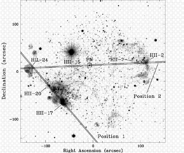
Figure 1: The combined H$\alpha$ image of Sextans A, obtained with the ESO NTT. North is up and East is to the left. The contrast is adjusted to highlight both bright and faint H$\alpha$ emission. Black objects on the image indicate bright sources. Long-slit orientations are shown; the slit width is 2″. The position of the PN is marked by a square. Only those H ii regions from Hodge, Kennicutt, & Strobel (1994) through which our slit positions passed are labeled. At the adopted distance of 1.32 Mpc, 1″ = 6.4 pc.

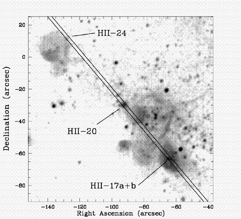
Figure 2: Enlargement of a portion of the combined H$\alpha$ image of Sextans A showing the H ii regions 24, 20, and 17 in more detail. The position of the 2″ width slit is marked. The H$\alpha$ image is rescaled to show the internal structure of H ii$-$17. Two compact bright knots, located on the rim of a circular shell, fall well inside the slit. The other shells are well resolved in the areas between H ii$-$20 and H ii$-$17, where H ii$-$16 18 and 19 (Hodge, Kennicutt, & Strobel, 1994) are located, and at the edge of H ii$-$24, where the slit is positioned.

For Sextans A we use the H ii region nomenclature published by Hodge, Kennicutt, & Strobel (1994). One of our slits crossed the extended regions H ii$-$17 and 19 and the compact region H ii$-$20 (see Figure 1 for more details). These H ii regions correspond to the regions 1, 3, and 2 of SKH89. Additionally, this slit position crossed the extended regions H ii$-$18, 22, and 24 (Hodge, Kennicutt, & Strobel, 1994). Thanks to the good seeing and resulting high angular resolution, $\sim$0$\farcs$5, H ii$-$17 was well resolved into two compact bright knots with an angular separation of $\sim$1$\farcs$5 (called hereafter H ii$-$17a and 17b), which seem to be located at the intersection of two shell-like structures (Figure 2). The second slit position went through the PN. The coordinates of the PN are given in Magrini et al. (2003), and a finding chart was published in Jacoby & Lesser (1981). This PN is called H ii$-$13 in Hodge, Kennicutt, & Strobel (1994). The second slit position also crosses H ii$-$2 and 7 in the West, H ii$-$15 in the central part of the galaxy, and the northern edge of H ii$-$24 in the East (see also Figure 1).

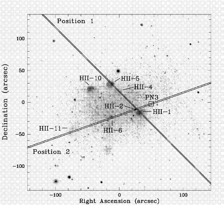
Figure 3: The NTT combined H$\alpha$ image of Sextans B. North is up and East is to the left. The contrast is adjusted to highlight both bright and faint H$\alpha$ emission. Black objects on the image indicate bright sources. Long-slit orientations are shown; the slit width is 2″. The position of PN3 is marked with a square. Labels indicate H ii regions from Strobel, Hodge, & Kennicutt (1991) through which the slits were positioned, or which were mentioned in the text. At the adopted distance of 1.36 Mpc, 1″ = 6.6 pc. The apparent line of emission in the upper right corner is an artifact resulting from CCD gaps in the mosaiced images.

In Sextans B we adopt the H ii region nomenclature suggested by Strobel, Hodge, & Kennicutt (1991). For the observed PN candidate in this galaxy we use the nomenclature of Magrini et al. (2002), who named it PN3. One slit position went through H ii$-$1, 4, 5, and the edge of 2, and the other one crossed H ii$-$2, 6, and 11 (see Figure 3 for more details).

2.3 Data reduction

The two-dimensional spectra were bias subtracted and flat-field corrected using IRAF. Cosmic ray removal was done with FILTER/COSMIC task in MIDAS. We use the IRAF software routines IDENTIFY, REIDENTIFY, FITCOORD, TRANSFORM to perform the wavelength calibration and to correct each frame for distortion and tilt. To derive the sensitivity curve, we fitted the observed spectral energy distribution of the standard stars with a high-order polynomial. All sensitivity curves observed during each night were compared and we found the final curves to have a precision better than 2% over the whole optical range, except for the region blueward of $\lambda$4000 where the sensitivity drops off rapidly. All two-dimensional spectra obtained with the same grism for the same object were averaged. One-dimensional (1D) spectra were then extracted from averaged frames using the IRAF APALL routine. For the H ii-regions 1D spectra were extracted from areas along the slit, where $I$($\lambda$4363 Å) $>$ 1.5$\sigma$ ($\sigma$ is the dispersion of the noise statistics around this line). For the PNe, 1D spectra were extracted to get the total light.

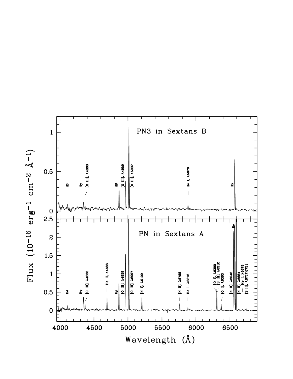
Figure 4: Emission-line spectra of the PN in Sextans A and PN3 in Sextans B from 4000 to 6900 Å, obtained with grism #5. The observed flux per unit wavelength is plotted versus wavelength. All detected emission lines are marked.

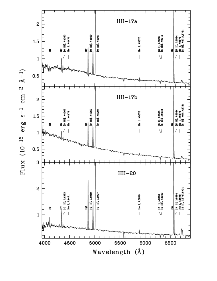
Figure 6: Emission-line spectra of H ii regions in Sextans A for which the [O iii] $\lambda$4363 line was detected, in the range from 4000 to 6900 Å, obtained with grism #5.

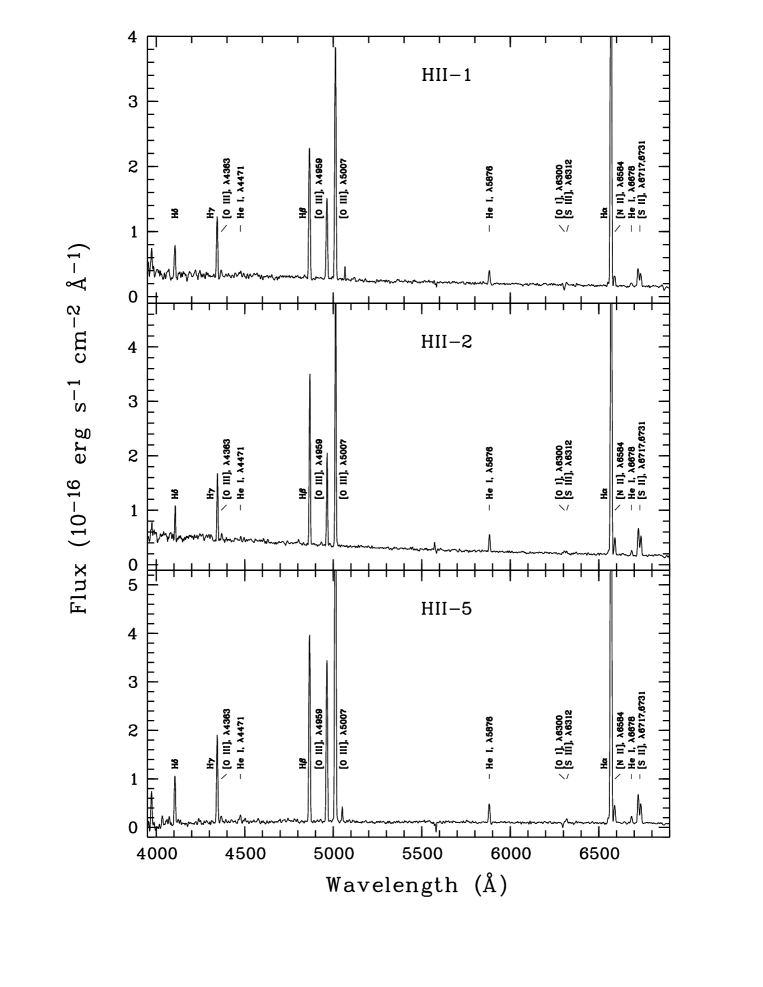
Figure 7: Emission-line spectra of H ii regions in Sextans B for which the [O iii] $\lambda$4363 line was detected, in the range from 4000 to 6900 Å, obtained with grism #5.

The resulting reduced and extracted spectra of the PNe in Sextans A and Sextans B obtained with grism #5 are shown in Fig. 4, and part of the reduced and extracted spectrum of the PN in Sextans A obtained with grism #6 is shown in Fig. 5. The reduced and extracted 1D spectra of H ii regions in Sextans A, obtained with grism #5 and in which the [O iii] $\lambda$4363 line was detected, are shown in Fig. 6. Fig. 7 shows the reduced and extracted 1D spectra obtained with grism #5 of H ii regions in Sextans B in which the [O iii] $\lambda$4363 line was detected.

After 1D-spectra were extracted, we used a method for measuring emission-line intensities described in detail in Kniazev et al. (2000a); Pustilnik et al. (2003); Kniazev et al. (2004): (1) the software is based on the MIDAS Command Language; (2) the continuum noise estimation was done using the absolute median deviation (AMD) estimator; (3) the continuum was determined with the algorithm from Shergin, Kniazev, & Lipovetsky (1996); (4) the programs dealing with the fitting of emission/absorption line parameters are based on the MIDAS FIT package; (5) every line was fitted with the Corrected Gauss-Newton method as a single Gaussian superimposed on the continuum-subtracted spectrum. Some close lines were fitted simultaneously as a blend of two or more Gaussian features: the H$\alpha$ $\lambda$6563 and [N ii] $\lambda\lambda$6548,6584 lines, [S ii] $\lambda\lambda$6716,6731 lines, and [O ii] $\lambda\lambda$7320,7330 lines; (6) the final errors in the line intensities, $\sigma_{\rm tot}$, include two components: $\sigma_{\rm p}$, due to the Poisson statistics of line photon flux, and $\sigma_{\rm c}$, the error resulting from the creation of the underlying continuum and calculated using the AMD estimator; (7) all uncertainties were propagated in the calculation of abundances and are accounted for in the accuracies of the presented element abundances.

The emission lines He i $\lambda$5876, [O i] $\lambda$6300, [S iii] $\lambda$6312, [O i] $\lambda$6364, H$\alpha$ $\lambda$6563, [N ii] $\lambda\lambda$6548,6584, He i $\lambda$6678, and [S ii] $\lambda\lambda$6716,6731 were usually detected independently in both grism spectra. Their intensities and equivalent widths were averaged after applying weights inversely proportional to the errors of the measurements.

2.4 Physical conditions and determination of heavy element abundances

The electron temperature, number densities, ionic and total element abundances for oxygen were calculated in the same manner as in Kniazev et al. (2004), where the [O ii] $\lambda$3727,3729 doublet was also not observed, and O⁺/H⁺ was calculated using intensities of the [O ii] $\lambda$7320,7330 lines. The contribution to the intensities of the [O ii] $\lambda$7320,7330 lines due to recombination was not taken into account since this is negligible compare to other uncertainties (namely, $<1\%$ as follows from Liu et al. (2000)). Total element abundances for Ne, N, S and Ar were derived after correction for unseen stages of ionization as described in Izotov, Thuan, & Lipovetsky (1994) and Thuan, Izotov, & Lipovetsky (1995): (1) the electron temperatures for different ions were either calculated from the relations in Garnett (1992) or using the equations following from the H ii photoionization models of Stasinska (1990):

$$t_{e}({\rm O\;II})=0.243+t_{e}({\rm O\;III})\left[1.031-0.184\,t_{e}({\rm O\;III})\right],$$ (1)

$$t_{e}(NeIII)=t_{e}(OIII),$$ (2)

$$t_{e}(NII)=t_{e}(OII),$$ (3)

$$t_{e}(SII)=t_{e}(OII),$$ (4)

$$t_{e}(ArIII)=0.83t_{e}(OIII)+0.17,$$ (5)

$$t_{e}(SIII)=t_{e}(ArIII),$$ (6)

$$t_{e}(ArIV)=t_{e}(OIII),$$ (7)

where t_e=T_e/10⁴K. (2) The ionization correction factors ICF(A) for different elements were calculated using the equations from Torres-Peimbert & Peimbert (1977); Garnett (1990); Izotov, Thuan, & Lipovetsky (1994); Thuan, Izotov, & Lipovetsky (1995):

$$ICF(N)=\frac{O}{O^{+}},$$ (8)

$$ICF(Ne)=\frac{O}{O^{++}},$$ (9)

$$ICF(S)=\frac{S}{S^{+}+S^{++}}=\{0.013+x[5.10+x(-12.78$$

$$+x(14.77-6.11x))]\}^{-1},$$ (10)

$$ICF(Ar)=\frac{Ar}{Ar^{++}+Ar^{+++}}$$

$$=\{0.99+x[0.091+x(-1.14+0.077x)]\}^{-1},$$ (11)

$$ICF(Ar)=\frac{Ar}{Ar^{++}}=[0.15+x(2.39-2.64x)]^{-1},$$ (12)

where $x$ = O⁺/O. In those cases where the [Ar iv] $\lambda$4740 line was not detected, equation 12 was used instead of equation 11. The He abundance was calculated following the method described in detail by Izotov, Thuan, & Lipovetsky (1997) and Izotov & Thuan (1998b).

The line [N ii] $\lambda$5755 was detected in the spectrum of the Sextans A PN, which allowed us to determine $t_{e}(NII)$ directly. This was done in the same way as for $t_{e}(OIII)$ using the Aller (1984) equation:

$$\frac{I(6584+6548)}{I(5755)}=C_{T}\Big{[}\frac{1+a_{1}x}{1+a_{2}x}\Big{]}10^{1.086/t_{\rm e}}$$ (13)

Here the constants $C_{T}$, $a_{1}$, and $a_{2}$ for different temperatures were taken from Aller (1984) and interpolated using an iterative procedure. $x=10^{-2}N_{e}T_{e}^{-1/2}$ is a term describing the dependence on the electron density $N_{e}$ and $T_{e}$.

Additionally, a strong nebular He II $\lambda$4686 emission line is detected in the spectrum of the Sextans A PN, implying the presence of a non-negligible amount of O³⁺. In this case its abundance was derived from the relation taken from Izotov & Thuan (1999):

$${\rm O}^{3+}=\frac{{\rm He}^{2+}}{{\rm He}^{+}}({\rm O}^{+}+{\rm O}^{2+})$$ (14)

After that, the total oxygen abundance is equal to

$${\rm O}={\rm O}^{+}+{\rm O}^{2+}+{\rm O}^{3+}$$ (15)

3 Results

3.1 Physical conditions and chemical abundances in H ii regions

The observed emission line intensities $F(\lambda)$, and those corrected for interstellar extinction and underlying stellar absorption $I(\lambda)$ are presented in Table 2 for the three H ii regions in Sextans A, in which the [O iii] $\lambda$4363 line was detected: H ii$-$17a, H ii$-$17b and H ii$-$20. The H$\beta$ equivalent width $EW$(H$\beta$), the absorption equivalent widths $EW$(abs) of the Balmer lines, the H$\beta$ flux, and the extinction coefficient $C$(H$\beta$) (this is a sum of the internal extinction in Sextans A and foreground extinction in the Milky Way) are also listed there. In Table 3 we present similar data for the three H ii regions H ii$-$1, 2 and 5 in Sextans B. The range of $C$(H$\beta$) measured in the H ii regions of Sextans A corresponds to values of B-band extinction A_B ranging from 0$\fm$20 to 0$\fm$54. Accounting for the Milky Way foreground extinction of 0$\fm$19 in the direction to this galaxy (Schlegel, Finkbeiner, & Davis, 1998) the internal extinction values are in the range of 0$\fm$01 to 0$\fm$35, implying a low dust content in these H ii regions. For Sextans B, the values of A_B calculated from the spectra for H ii$-$5 and 1 are consistent to within the uncertainty in the foreground extinction in the direction of this galaxy, 0$\fm$14. The A_B for H ii$-$2 corresponds to an additional internal extinction of 0$\fm$35.

In Table 4 we give the derived physical conditions and ion and element abundances for the above mentioned three H ii regions in Sextans A. The corresponding data for three H ii regions in Sextans B are presented in Table 5. As evident from these Tables, we detected the faint [O iii] $\lambda$4363 line at the level of 4 to 8 $\sigma_{\rm noise}$ and the [O ii] $\lambda$7325 line at the level of 4 to 10 $\sigma_{\rm noise}$. This results in O/H uncertainties in the individual H ii regions on the order of 0.05 to 0.11 dex. Since the flux uncertainties of faint lines of other ions are in general higher, the resulting errors of N/H, S/H and Ar/H in the individual H ii regions lie in the range of 0.1 to 0.2 dex. The line [S iii] $\lambda$6312 is not detected in H ii$-$17b of Sextans A, and the derived value of S/H should therefore be treated as a lower limit. Hence we do not list S/H for this H ii region. The line [Ne iii] $\lambda$3868 is detected in only one H ii region, due to the significant drop in sensitivity below $\sim$$\lambda$4000 Å.

All three H ii regions in Sextans A from Table 4 show oxygen abundances consistent with each other to within the uncertainties, and hence a weighted average value of 12+log(O/H)=7.54$\pm$0.06 can be derived for this galaxy based on our data. For the two H ii regions in Sextans B (H ii$-$1 and H ii$-$2 from Table 5), the oxygen abundances also are very similar and within their rather small rms uncertainties can be treated as equal. Their weighted mean O/H value corresponds to 12+$\log$(O/H)=7.53$\pm$0.05.

The average relative abundances N/O, S/O and Ar/O for all three H ii regions in Sextans A ($-$1.58$\pm$0.07, $-$1.45$\pm$0.18, and $-$2.06$\pm$0.09 respectively) and for two low-metallicity H ii regions in Sextans B ($-$1.53$\pm$0.07, $-$1.59$\pm$0.09, and $-$2.04$\pm$0.06) are quite consistent with the average values for the most metal-poor H ii galaxies obtained by Izotov & Thuan (1999) and confirmed in many subsequent observations (e.g., Kniazev et al., 2000a, b; Guseva et al., 2001, 2003a, 2003b, 2003c; Pustilnik et al., 2003, 2004), implying production in massive stars. The relative abundances of N/O, Ne/O, S/O and Ar/O for the third H ii region in Sextans B analyzed here are also consistent with the mean values determined by Izotov & Thuan (1999) for their high-metallicity subsample of H ii galaxies.

3.2 Physical conditions and elemental abundances in PNe

We present the observed and Balmer line extinction corrected emission line intensities for the two observed PNe in Table 6. Our fluxes for the emission lines [O iii] $\lambda$5007 and H$\alpha$ in both PNe are consistent to within the observational uncertainties with the fluxes measured by Magrini et al. (2003) and Magrini et al. (2002). The measured $C$(H$\beta$) in the Sextans A and Sextans B PNe corresponds to A_B of 0$\fm$66 and 0$\fm$71, respectively (A_V of 0$\fm$50 and 0$\fm$54). After accounting for the Galactic contribution, this suggests an intrinsic extinction A_B of 0$\fm$47 and 0$\fm$57, which is higher than the values for H ii regions in these galaxies. This result is consistent with the fact that the progenitors of PNe produce additional dust in the late stages of their evolution. In Table 7 we give the derived physical conditions, ion and element abundances for both PNe.

For the PN in Sextans A the quality of the spectral data is comparable to the quality of the H ii region spectra. The resulting uncertainties in He/H, O/H and N/H are at the level of 0.03–0.05 dex. The values of O/H and N/H for the PN appear to be significantly higher than observed in the H ii regions of this galaxy (by a factor of $\sim$3 and $\sim$250, respectively). With $\log$(N/O) = 0.39 and He/H = 0.107$\pm$0.008, according to the definition of Kingsburgh & Barlow (1994, $\log$(N/O)$>-$0.1) or to the definition in Leisy & Dennefeld (1996, $\log$(N/O)$>-$0.6 and He/H $>$ 0.10), the PN in Sextans A should be classified as a Type I.

Since the line fluxes of PN3 in Sextans B are about a factor of 2–3 (apart [N ii]) lower than for the Sextans A PN, the resulting signal-to-noise for the spectrum of PN3 in Sextans B is significantly less. Therefore, from this spectrum it was only possible to derive values of O/H and N/H with final uncertainties of 0.16 and 0.18 dex, respectively. The observed properties of PN3 allow us to exclude a classification as a PN of Type I. However, the quality of the PN spectrum is not sufficient to perform the detailed comparison of its abundances with those of the H ii regions in Sextans B.

3.3 Physical Parameters of observed PNe

The self-consistent age-dating of PNe progenitors requires the determination of the bolometric luminosity and the effective temperature of the PN central star in combination with photoionization modelling and PN evolutionary tracks (Dopita et al., 1997). This is well beyond the scope of our paper. However, based on our data, it is possible to make some rough estimates, which we summarize in Table Spectrophotometry of Sextans A and B: Chemical Abundances of H ii Regions and Planetary Nebulae. The effective temperatures (T_eff) of the PN progenitors can be estimated by the method developed by Zanstra (1927). Since the method is applicable for the case of optically thick nebulae, we have to first check whether our PNe are optically thick. The criteria of this were suggested by Kaler (1983) on the results of analysis of the dereddened I(3727)/I(H$\beta$), I(4686)/I(H$\beta$) and I(6584)/I(H$\alpha$) line ratios for the large sample of PNe covered a wide range of optical thickness. According to these criteria, the dereddened line ratios I(4686)/I(H$\beta$) and I(6584)/I(H$\alpha$) that reflect the Zanstra temperature ratio TR=T_z(He ii)/T_z(H) (Kaler, 1983), show that our PNe are certainly optically thick, since: (a) PN in Sextans A has TR$\leq$1.2 and is the Case 1 following Kaler (1983) classification (class a i from Seaton, 1966); (b) PN3 in Sextans B has TR$>$1.2 and I(4686)$<$0.9 and is the Case 2 following Kaler (1983) classification (class a ii from Seaton, 1966). From the spectrum of PN3 in Sextans B we estimated a 2$\sigma$ upper limit for the flux of He ii $\lambda$4686 line as 8% of I(H$\beta$). After that, for the calculation of the Zanstra temperature we used the equation suggested by Kaler & Jacoby (1989):

$$\log{T_{eff}}=4.905+1.11162\times 10^{-2}I_{c}(\lambda 4686)$$

$$-1.10692\times 10^{-4}I_{c}^{2}(\lambda 4686)$$

$$+6.20572\times 10^{-7}I_{c}^{3}(\lambda 4686),$$ (16)

where $I_{c}(\lambda 4686)$ is the flux of He ii $\lambda$4686 in the units of I(H$\beta$) with I(H$\beta$) = 100.

The total luminosities of the PN central stars were derived from the relation given in Gathier & Pottash (1989); Zijlstra & Pottasch (1989), using the H$\beta$ absolute fluxes, extinction $C$(H$\beta$) and distances:

$$L=150\times L(H\beta)$$ (17)

Masses were derived from the theoretical evolutionary tracks of Vassiliadis & Wood (1994) for Z=0.001 (1/20 of Z_⊙). The ages were derived using the evolutionary lifetimes of the various phases of the progenitor stars from Vassiliadis & Wood (1993), also for Z=0.001.

In addition, since the PNe 1D spectra were extracted taking the total light of a nebula, we synthesized the $VRI$ colors of the PNe using zeropoints from the spectrum of Vega (Castelli & Kurucz, 1996). These colors were transformed into the standard Johnson-Cousins $UBVRI$ system as specified by Bessel (1990) and Bessel, Castelli, & Plez (1998). The $B$-band was not included in Table Spectrophotometry of Sextans A and B: Chemical Abundances of H ii Regions and Planetary Nebulae since, due to the drop in sensitivity, the spectra become very noisy below $\sim$$\lambda$4000 Å.

4 Discussion

4.1 PN abundances vs. H ii region abundances

H ii region abundances mainly provide information about $\alpha$-process elements, produced predominantly in short-lived massive stars. In contrast to H ii regions, some elemental abundances in PNe are affected by nucleosynthesis in the PN progenitor stars. It is well known that newly synthesized material can be dredged up by convection in the envelope, significantly altering the abundances of He, C, and N in the surface layers during the evolution of 1–8 M_⊙ stars on the giant branch and asymptotic giant branch (AGB; Leisy & Dennefeld, 1996; Boothroyd & Sackmann, 1999; Henry, Kwitter, & Bates, 2000). In addition, if during the thermally pulsing phase of AGB evolution convection “overshoots” into the core, significant amounts of ¹⁶O can be mixed into the inter-shell region and may be convected to the surface (Herwig, 2000; Blöcker, 2003). In combination, all of the above factors mean that only the Ne, S, and Ar abundances, observed in both H ii regions and PNe, can be considered as reliable probes of the enrichment history of galaxies, unaffected by the immediately preceding nucleosynthesis in the progenitor stars. Therefore, in further discussions of PN progenitor metallicity we do not use O/H, He/H, and N/H as reliable metallicity indicators and base our conclusions on chemical evolution only on PNe abundances of Ne, S, and Ar.

4.2 Observed heavy element abundances

4.2.1 Sextans A abundances

The value of 12+log(O/H)=7.54$\pm$0.06, derived here as the average of three H ii regions in Sextans A, is in good agreement with the earlier derived value 12+log(O/H)=7.49$\pm$0.3 from SKH89. However, the previous value was based on spectra of four separate H ii regions with only a marginal detection of [O iii] $\lambda$4363 in one of them, such that SKH89 used a combined estimate for all four H ii regions based on the strong-line empirical relation of Pagel et al. (1989). It is worth noting that the use of modern empirical calibrations of the strong-line relation (McGaugh, 1991; Pilyugin, 2001) for the published data from SKH89 gives 12+$\log$(O/H) in the range of 7.7 to 8.0.

Recently Kaufer et al. (2004) measured the present-day stellar metallicity of Sextans A using three A-type supergiants with ages of $\sim$10 Myr. Their average $\alpha$-element abundance, derived from Mg I lines, relative to the solar value is $<$[$\alpha$(Mg I)/H]$>$ = –1.09 $\pm$ 0.02 $\pm$0.19, which corresponds to an oxygen abundance of 12+$\log$(O/H) = 7.57 dex. This is in excellent agreement with our average O/H for the three H ii regions, which are roughly located in the same part of Sextans A. Thus, the element abundances in these H ii regions and in the three A supergiants located in other parts of Sextans A (see Figure 1 from Kaufer et al., 2004) do not provide any evidence of metallicity inhomogeneity in this galaxy.

Since the abundances of the $\alpha$-elements S and Ar in the Sextans A PN should not be affected by nucleosynthesis in its progenitor star, these elements can be used as good tracers of the metallicity of the interstellar gas in Sextans A at the epoch when the PN progenitor was formed. According to our estimate, this occurred some 1.6 Gyr ago (Table Spectrophotometry of Sextans A and B: Chemical Abundances of H ii Regions and Planetary Nebulae). Due to the limited accuracy of S/H and Ar/H in the H ii regions, and especially in the PN (in the latter the errors are on the order of about 40% – 50%), the quantitative result on the rate of the interstellar medium (ISM) enrichment needs further improvement. However, the values for relative enrichment, derived independently for sulfur, (S/H)_HII/(S/H)_PN = 3.17 ($\pm^{1.9}_{0.87}$)$\pm$1.05, and argon, (Ar/H)_HII/(Ar/H)_PN = 2.99 ($\pm^{2.83}_{0.98}$)$\pm$0.54, are consistent with each other. We give the estimates of the uncertainties of these ratios in the above form since, due to the large relative errors of the values in the denominators, 1$\sigma$ intervals are highly non-symmetric; the values in parenthesis give the uncertainties in the denominators, while the last term describes the uncertainties in the numerators. The weighted average value is $\sim$3.1$\pm^{2}_{1}$ or equivalently, 0.5$\pm$0.2 dex.

This rather large enrichment in $\alpha$-elements may be caused by the increase in the star formation rate during the last $\sim$1–2 Gyr. When we transform the above values to O/H and take the $\alpha$-element enrichment into account, we find 12+$\log$(O/H)${}_{\rm(-2~{}Gyr)}$ = 7.04$\pm$0.20 as the value prior to enrichment. The comparison of element abundances in three H ii regions and in the PN suggests that the region of Sextans A where the PN progenitor formed was as metal-deficient as I Zw 18 is now (Skillman & Kennicutt, 1993; Izotov & Thuan, 1998a; Kniazev et al., 2003). Moreover, assuming the element abundance pattern in the gas of which the PN progenitor formed to be typical of very low-metallicity H ii galaxies, we conclude that the progenitor star, with an estimated mass of 1.5M_⊙, enriched the material of this PN by a factor of $\sim$10 in oxygen (from the value of 12+$\log$(O/H)=7.04 to the current value of 8.02), and by a factor of $\sim$750 in nitrogen.

4.2.2 Sextans B abundances

Previously, Stasinska, Comte & Vigroux (1986) observed, according to their description, H ii$-$5 (although the object indicated on their finding chart seems to be closer to H ii$-$10). They did not detect [O iii] $\lambda$4363 and presented a lower limit on O/H, equivalent to 12+$\log$(O/H)$\geq$7.4. Later, four H ii regions (H ii$-$1, 2, 5, and 10) were observed by SKH89. These authors failed to detect [O iii] $\lambda$4363. To determine O/H, they used the empirical strong lines relation (which has an internal accuracy of 50%) by Pagel et al. (1989) and derived a lower limit for O/H in H ii$-$5. Their resulting value for the oxygen abundance of Sextans B was 12+$\log$(O/H)=7.56. Subsequently, MAM90 detected [O iii] $\lambda$4363 in the spectrum of H ii$-$5 at a level of 0.021$\pm$0.005 of I(H$\beta$) and derived its O/H as 12+$\log$(O/H)=8.12, with no cited uncertainty. We estimate that their rms is $\geq 0.1$ dex. It is worth noting here that the empirical value of SKH89 for H ii$-$5 is not in good agreement with the value derived via the T_e-method in MAM90. In his compilation, Mateo (1998) adopted an average value of 12+$\log$(O/H)=7.84$\pm$0.3 for Sextans B.

In our observations of Sextans B H ii regions, the temperature-sensitive line [O iii] $\lambda$4363 was detected, and hence O/H was reliably measured, in only three of them. For H ii$-$1 and H ii$-$2, which are next to each other and which are situated at the western part of the brighter central one-kpc region (Figure 3), the oxygen and other element abundances are very similar. For the third H ii region (H ii$-$5 in Figure 3, at $\sim$0.6 kpc NE) the oxygen abundance (12+$\log$(O/H)=7.84$\pm$0.05) is larger than for the former two by a factor of 2.05$\pm$0.35. The ratios of the other elements are similar: (N/H)_HII-5/(N/H)${}_{\rm HII-1,2}=2.40\pm 0.55$, (Ar/H)_HII-5/(Ar/H)${}_{\rm HII-1,2}=2.89\pm 0.50$, and (S/H)_HII-5/(S/H)${}_{\rm HII-1,2}=3.33\pm 0.8$. All these ratios are consistent to within their rms uncertainties. Their mean abundances imply an enrichment by a factor of $\sim$2.5 relative to the element abundances in H ii$-$1 and 2. These differences are significant for each of the four elements at a confidence level corresponding to 4 $\sigma_{\rm comb}$, where $\sigma_{\rm comb}$ is the combined rms error of the difference (on a linear scale) between the abundances in H ii$-$5 and the average on H ii$-$1 and 2.

We have checked whether our results for H ii$-$5 are consistent with the O/H value from MAM90. For this we recalculated their O/H in our system, using their relative line intensities, and obtained 12+$\log$(O/H)=8.06. This is consistent with our value to within $\sim$2$\sigma_{\rm comb}$. The main difference comes from our higher (by a factor of 1.5) relative intensity of [O iii] $\lambda$4363, which is detected in our spectrum at an 8$\sigma$ level compared to a 4$\sigma$ detection in MAM90. Therefore, we consider our element abundances to be more reliable. We also note that the apparent problem with the small value of $\log$(N/O) = $-$1.8 in this H ii region that was pointed out by Skillman, Bomans, & Kobulnicky (1997) from the data of MAM90, does not exist according to our data.

While the disagreement between the O/H values of SKH89 and MAM90 could (in principle) be considered as an indication of O/H inhomogeneity, our data provide the first firm evidence of such chemical inhomogeneity in the interstellar medium of Sextans B on scales of $\sim$0.5–1 kpc.

In contrast to the PN in Sextans A, the accuracy of the O/H and N/H ratios measured in PN3 in Sextans B allows us to formulate only very preliminary conclusions. O/H and N/H in this PN are very close to the average values derived for Sextans B H ii regions 1 and 2 (the difference is $\lesssim$0.5 $\sigma_{\rm comb}$). The measured relative abundance log(N/O) = –1.48$\pm$0.24 for this PN is well consistent with the average values for the most metal-poor H ii galaxies (Izotov & Thuan, 1999). This suggests that the enrichment in O and N is sufficiently small and in general does not exceed the uncertainty of log(N/O). Adopting the 95% confidence level for the possible O and N abundances in PN3, we conclude that the maximum O and N enrichment since the epoch of the PN progenitor’s formation does not exceed $\sim$0.4 dex.

4.3 Chemical inhomogeneities in dwarf irregular galaxies

Summarizing the results on the element abundances in Sextans B, we conclude that our new spectroscopy confirms earlier conclusions (based on lower accuracy measurements) that some of the nearby dIrr galaxies reveal considerable abundance inhomogeneities among their H ii regions. This is an important finding since dIrr galaxies are usually believed to be chemically well-mixed and homogeneous at a given age. To confidently determine the average ISM metallicity in a well-resolved dIrr galaxy one thus needs to measure its abundances in several regions. Various processes (such as metal-enriched outflows, self-enrichment on a time-scale of a few Myr, or infalling metal-poor intergalactic HI clouds) can in principle be responsible for the local deviations of the ISM metallicity from some average galactic value. They may result in either an excess or a deficiency as compared to the galactic mean. Note that in the lower-mass dwarf spheroidal galaxies there are indications for chemical inhomogeneities in terms of possible radial gradients among their old stellar populations (Harbeck et al., 2001). The available data on H ii regions of Sextans B, taken at face value, are inconclusive in terms of constraining the probable cause of the inhomogeneities. It is unfortunate that older tracers of the chemical evolutionary history of galaxies like Sextans B are so difficult to measure. For the time being, only photometric estimates are available for the old population(s), based either on isochrones or on globular cluster red giant branch fiducials. For Sextans B it would be useful to observe more H ii regions at a sufficient depth to detect the [O iii] $\lambda$4363 line, in order to explore what level of present-day metallicity is characteristic of the entire galaxy. The other three H ii regions visible in our long-slit spectra will require observations with an 8-m class telescope to reach an adequate signal to noise level.

It is worth noting that the census of H ii region metallicities in dIrr galaxies in the LG and its surroundings is rather unsatisfactory. Only in the Magellanic Clouds can the number and spatial extent of H ii regions with measured element abundances be considered sufficient for investigations of the chemical inhomogeneity problem (see, e.g., Pagel et al., 1978; Vermeij & van der Hulst, 2003). But even in the SMC, the situation could be improved; while in the former study 19 H ii regions were studied across much of the radial extent of the Clouds, $\sim$5^∘ ($\sim$5 kpc), the uncertainties of the individual O/H values seem too large to exclude possible variations at the level of $\sim$0.3 dex (this level of variations we see in Sextans B). In the latter study the errors of O/H are reasonably small, and they are consistent for all three measured H ii regions to within 20% (or 0.08 dex), but all three regions are located close to each other within a circle $\sim$20 pc in diameter.

For most of the other nearby dIrr galaxies, O/H values are based on old data, generally of poor to moderate signal to noise for [O iii] $\lambda$4363. Alternatively (or in addition), in many cases only one to two H ii regions per galaxy were measured (e.g., Pagel et al., 1978; Skillman, Kennicutt & Hodge, 1989; Skillman, Terlevich & Melnick, 1989; Moles, Aparicio, & Masegosa, 1990; Hodge & Miller, 1995; Lee, Grebel, & Hodge, 2003a; Lee et al., 2003b). Thus the existing data for most nearby dIrr galaxies do not allow one to draw a definite conclusion on chemical inhomogeneities in the ISM at a level of $\sim$0.3 dex across the entire galaxy. The general claim by Mateo (1998) that there is “no evidence for significant dispersion of oxygen abundances in any Local Group dIrrs in which multiple H ii regions have been studied” should therefore be treated with some caution; this statement probably applies only to variations with an amplitude of $\sim$0.4 dex or higher. We are aware of only a few similar occurrences in nearby dIrr galaxies: in the LG dIrr galaxies SMC and WLM and in the M 81 group dwarf Holmberg II. Star clusters in the SMC appear to differ in their metallicity at a given age (Da Costa, 2002), which seems to indicate differences in the chemical composition in different regions of this galaxies at a given time. In WLM, Venn et al. (2003) discovered that one of two studied blue supergiants has a clearly higher [O/H] than the value measured for the H ii region WLM HM$-$7, situated 300 pc away from this star. The supergiant exceeds the [O/H] of the ISM by $\approx$0.7 dex at a 3$\sigma$ level, a curious difference for which an explanation still needs to be found (Lee, Skillman, & Venn, 2005). For Holmberg II we estimated from the data of Lee et al. (2003b) that the weighted average of 12+$\log$(O/H) for four H ii regions where [O iii] $\lambda$4363 was measured is 7.63$\pm$0.08, while for the H II$-$6 region the 2$\sigma$ lower limit is indicated as 7.97; in this galaxy several H ii regions show low abundances, while one appears to be enriched by a factor of $\sim$2.

Roy & Kunth (1995), in their analysis of dispersal and mixing of oxygen in the ISM of gas-rich galaxies, gave a fairly low characteristic time of 1.5 Myr for local mixing of freshly ejected nucleosynthesis products due to Raleigh-Taylor and Kelvin-Helmholtz instabilities in star-forming regions. While these processes are likely to be very efficient in mixing freshly released processed heavy elements into the ambient ISM, detailed numerical simulations would be desirable that take the specific conditions in our target galaxies into account. In their analysis of a large sample of H ii galaxies, Stasinska & Izotov (2003) also conclude that some self-enrichment should play a role in these objects in order to match all observed correlations.

Galaxies of different types generally follow a trend of increased global metallicity with increased luminosity, although offsets exist between different galaxy types (e.g., Grebel, Gallagher, & Harbeck, 2003, GGH03 hereafter). The lower O/H in two H ii regions of Sextans B gives a better agreement with the empirical relation between O/H and the blue luminosity for dwarf irregular galaxies (e.g., SKH89), while the higher value of O/H in the H ii$-$5 region shifts Sextans B well above the 12+$\log$(O/H) vs $L_{\rm B}$ relation. Thus, the hypothesis of a significant overabundance in the region H ii$-$5, related to localized metal pollution, sounds more realistic. However, as discussed earlier, so far such cases appear to be quite rare. This is in some aspects similar to the detection of a significant nitrogen overabundance (on the spatial scale of $\sim$50 pc) in the central starburst of a nearby dwarf starburst galaxy, NGC 5253 (Kobulnicky et al., 1997), again supporting very short characteristic timescales of local enrichment and subsequent dispersal as suggested by Roy & Kunth (1995). This may then imply that we caught the evolution of H ii$-$5 during the short period when fresh $\alpha$-elements were just mixed into the $\sim$10⁴ K medium via stellar winds and supernova ejecta, but prior to their dilution via the mechanisms discussed, e.g., by Roy & Kunth (1995) and Tenorio-Tagle (1996).

If this is the case, the detection of chemical inhomogeneities in the star-forming regions across the body of a dwarf galaxy is facilitated by the high spatial resolution of our study ($\sim$6 pc), which avoids the effective smearing of the localized short time-scale enrichment in more distant actively star-forming galaxies due to limited angular/spatial resolution. Obviously, this also implies that galaxies with many H ii regions offer a better chance to detect inhomogeneities than dIrrs with only one or two H ii regions.

In order to better understand possible reasons for the observed metal excess in H ii$-$5, more detailed and higher angular resolution studies of this region would be helpful. If the excess is indeed related to the recent effective mixing of the H ii region’s gas with matter from a hot bubble, some tracers of such a process could be imprinted in the ionized gas kinematics, or in additional ionization and excitation compared to more typical cases.

4.4 Chemical evolution: Photometry versus spectroscopy

4.4.1 Sextans A

How do the spectroscopic results compare with the photometric enrichment history derived by Dolphin et al. (2003b)? Using synthetic color-magnitude diagram (CMD) techniques, these authors found a fairly constant average stellar metallicity throughout the galaxy’s history of [Fe/H] $\approx$ $-$1.45$\pm$0.2. They suggest that most of the enrichment occurred more than 10 Gyr ago. For the old red giant branch GGH03 quote an approximate photometric mean metallicity of $-1.9$ dex, estimated from comparison with globular cluster red giant branch fiducials. Dolphin et al. (2003b)’s star formation history implies that more than half of the stellar mass formed during that early period. However, Dolphin et al. (2003b) also caution that the early star formation history cannot be accurately inferred from the available HST data. Approximately 10 Gyr ago the average star formation (SF hereafter) rate dropped for a period of $\sim$7.5 Gyr by a factor of $\sim$20 with only about 5% of all stellar mass forming during that intermediate-age period. Presumably, the low SF intensity would have been accompanied by little chemical enrichment. About 1–2 Gyr ago the SF again increased drastically, resulting in the formation of about 30% of the stellar mass of Sextans A. This latter episode of active star formation should have been accompanied by a significant production of metals.

The present-day spectroscopic metallicity of [Fe/H] $\approx$ $-$1.1 dex (from H ii regions and young A supergiants) is consistent with an enrichment of about 0.4 dex compared to the average stellar metallicity from Dolphin et al. (2003b), and with an enrichment of $\sim 0.8$ dex compared to the mean metallicity of the old red giants in Sextans A (Grebel, Gallagher, & Harbeck, 2003). One cannot exclude, however, that due to the powerful energy release over the period of increased star formation during the past 1–2 Gyr a significant fraction of freshly synthesized heavy elements was blown away. Thus, the metallicity in the young population and ISM may indicate only a lower limit of the true metal production during this period.

In the above scenario, the results for the star formation history and metal enrichment of Sextans A, derived from photometric data, are compatible with our conclusion of 0.5$\pm$0.2 dex enrichment according to the comparison of the H ii region abundances and the data on S and Ar abundances in the sole PN of Sextans A. As we show in Table Spectrophotometry of Sextans A and B: Chemical Abundances of H ii Regions and Planetary Nebulae the PN progenitor was a low-mass star with $\sim$1.5 M_⊙ and an age of $\sim$1.6 Gyr, i.e., it formed at that time when the star formation rate and the accompanying enrichment showed a marked increase, according to Dolphin et al. (2003b).

4.4.2 Sextans B

For Sextans B, the deepest published CMD is based on HST data (Karachentsev et al., 2002c) but only covers the upper red giant branch. Hence no attempt was made to derive the star formation history of Sextans B from these data. However, the CMD of Karachentsev et al. (2002c) allows us to draw the following qualitative conclusions: Sextans B possesses a substantial intermediate-age to old population with ages exceeding $\sim 2$ Gyr as evidenced by its very well populated, prominent red giant branch. Our estimate of the age of the observed PN progenitor (see Table Spectrophotometry of Sextans A and B: Chemical Abundances of H ii Regions and Planetary Nebulae) also supports the idea that Sextans B had increased SF about 6 Gyr ago. GGH03 suggest a mean photometric metallicity of $-2.1$ dex for the old population through comparison of the red giant branch with globular cluster fiducials. The CMD of Karachentsev et al. (2002c) also shows the presence of a large number of luminous asymptotic giant branch stars above the tip of the red giant branch, and an extended group of young blue main-sequence stars and blue-loop stars. Red supergiants appear to be present as well. To summarize, the CMD shows the typical features also known from many other dIrr galaxies, which support the scenario of star formation continuing over a Hubble time (e.g., Grebel 1999). In earlier work based on much shallower ground-based data, Tosi et al. (1991) studied the recent star formation history of Sextans B up to 1 Gyr and found moderate star formation activity, probably intermittent. They provide a rough photometric estimate of the young population’s stellar metallicity of $-1.3$ dex. While they claim that the oxygen abundance in the H ii$-$10 region of 12+$\log$(O/H)=8.1 (MAM90) is in the perfect agreement with their stellar metallicity estimate, this is no longer correct. In the modern calibration the above oxygen abundance corresponds to [O/H]=$-$0.65. The current ISM metallicity, as measured here by O/H in the two low-metallicity H ii regions, corresponds to [O/H] = $-$1.13$\pm$0.07. The latter, however, is in agreement with the estimate of the young population’s stellar metallicity from Tosi et al. (1991). We estimated in Section 4.2.2 that the maximum O and N enrichment during the last few Gyr does not exceed $\sim$0.4 dex for Sextans B. If this is true, one can suggest that most of the enrichment occured in Sextans B more than 6 Gyr ago, as would also be suggested by the very low metallicity of the old red giant branch in Sextans B derived by GGH03.

The qualitative star formation history of Sextans B over the total cosmological time, based on all previously available CMD data is summarized by Grebel (1997), Mateo (1998), and Grebel (1999). It may have shown a pronounced early star formation rate during the first few Gyr with a subsequent period of possibly lower star formation activity and a potential increase at more recent times (say, 1–2 Gyr ago). It should be emphasized that there is still very little quantitative information on the star formation history of Sextans B.

4.5 Sextans A versus Sextans B SF histories

The general similarity of the SF histories of both Sextans A and B and other nearby dwarf irregulars is important in the aspect of dwarf galaxy evolution in small galaxy groups. This likely implies that the SF drivers are similar in the LG and this particular dwarf group. Another question concerns the nature of significant differences in SF histories during the last several Gyr; since there appears to be little correlation between the SF histories of Sextans A and B, it is tempting to suggest that the SF during this period was mainly due to intrinsic processes, unrelated to the tidal action from a nearby neighbor. Indeed, the estimate of tidal forces between the two dwarfs, based on their projected distance of $\sim$250 pc, total masses of $\sim$(4–8)$\times$10⁸ M_⊙ and Holmberg radii of $\sim$0.8–0.9 kpc (Mateo, 1998) results in a relative strength of tides of the order of 10^-7. However, this issue needs more careful study including the morphology and kinematics of gas and stars in these galaxies, and more importantly, constraints on their orbits.

While the SF histories of dwarf galaxies of the same morphological type exhibit similar overall properties and trends, they differ in the details. Indeed, each dwarf has its own unique evolutionary history (e.g., Grebel 1997). These differences become most pronounced on scales of a fraction of a Gyr, but may encompass time scales of several Gyr. In the absence of detailed, deep CMDs and detailed information on the chemical evolution of such galaxies, the PN census may serve as a possible indicator. Since the absolute magnitudes $M_{\rm B}$ of Sextans A and B are very similar (see Table Spectrophotometry of Sextans A and B: Chemical Abundances of H ii Regions and Planetary Nebulae), and since their global SF histories appear to be similar, we should then expect that both galaxies also have a comparable number of PNe. Instead, surveys for PNe in the two dIrrs have revealed a difference by a factor of 5 in the PN census. This may imply that Sextans B experienced a significantly higher SF rate during the aforementioned time interval. Similar conclusions the likely differing SF histories in Sextans A and B during last few Gyr were reached by Magrini et al. (2002, 2003, 2004).

5 Summary and conclusions

In this paper we presented new determinations of the chemical abundances of six H ii regions in Sextans A and B, and of one PN in each of these galaxies. Based on the data and discussion presented in the paper, the following conclusions can be drawn:

1. We confirmed with good accuracy the low ISM metallicity of both galaxies, with 12+$\log$(O/H) = 7.54$\pm$0.06 in three H ii regions in Sextans A, and 12+$\log$(O/H) = 7.53$\pm$0.05 in two H ii regions in Sextans B. The element abundance ratios of O, N, S, and Ar are well consistent with the expected patterns of very metal-poor H ii galaxies.

2. New high accuracy chemical abundances in the H ii regions of Sextans A and B allowed us to probe the present-day metallicity homogeneity across the bodies of the respective galaxies. While our statistics are still poor (three H ii regions per galaxy), we find that in Sextans A the measured abundances in all three H ii regions show no differences exceeding 0.1 dex (at the 63% confidence level). Moreover, the metallicities of three A-supergiants studied by Kaufer et al. (2004) are in good agreement with those of the H ii regions.

3. In Sextans B one H ii region (H ii$-$5) is significantly enriched, with an excess in O, N, S, and Ar of a factor of 2.5$\pm$0.5 relative to the mean value of the two other H ii regions studied here. This is strong evidence for chemical inhomogeneity in a dIrr galaxy. Whether this implies a general chemical inhomogeneity among populations of comparable age in Sextans B, and thus a metallicity spread at a given age, or whether we happen to see the short-lived effects of freshly ejected nucleosynthesis products prior to their dispersal and mixing with the ambient interstellar medium will require further study.

4. Chemical abundances derived for the PN in Sextans A show that this is a Type I object with a highly elevated nitrogen abundance: N/O $\sim$2.5. Its O/H is about a factor of 3 higher than in the H ii regions, which implies significant self-pollution by the PN progenitor. The abundances of S and Ar indicate that the ISM metallicity was $\sim$0.5 dex lower at the time of the formation of the PN progenitor, compared to that currently measured in H ii regions. In this case the PN progenitor enriched the material by a factor of $\sim$10 in oxygen, and by a factor of $\sim$750 in nitrogen.

5. The element abundances of PN3 in Sextans B are consistent with those of the two H ii regions with low metallicity. Comparison of the element abundances for this PN and the two nearby H ii regions implies that the maximum O and N enrichment during the last few Gyr (the estimated age of the progenitor star of PN3) did not exceed $\sim$0.4 dex.

6. Despite the overall similarity of Sextans A and B, their star formation history and enrichment history over the last few Gyr looks quite different, as evidenced by both the number of H ii regions and PNe, and their abundances. The overall chemical enrichment experienced by Sextans A and B as judged from the estimated mean metallicity of their old red giant branch populations and their H ii regions has spanned at least 0.8 dex. This number is a lower limit since it refers to the mean red giant metallicity and necessarily neglects the still unknown metallicity of the most metal-poor giants in the two dIrrs.

Figure 5: Emission-line spectrum of the PN in Sextans A from 5800 to 7800 Å, obtained with grism #6.

Table 1: Basic Parameters of the Sextans A and Sextans B Dwarf Irregular Galaxies

Property	Sextans A	Sextans B
(1)	(2)	(3)
Alternate Names	UGCA 205, DDO 75	UGC 5373, DDO 70
$\alpha$ (J2000.0)	10h11m00.80s	10h00m00.10s
$\delta$ (J2000.0)	$-$04∘41′34.0′′	+05∘19′56.0′′
Distance (kpc)	1320$\pm$401	1360$\pm$702
V⊙,opt (km s${}^{-}{1}$)	328$\pm$53	301$\pm$15
V⊙,radio (km s${}^{-}{1}$)	325$\pm$34	303$\pm$26
BT (mag)	11.867	11.852
AB (mag)a	0.19	0.14
(m-M0) (mag)	25.627	25.677
MB	$-13.96$	$-13.97$

References. — (1) Dolphin et al. (2003a); (2) Karachentsev et al. (2002c); (3) Tomita, Ohta, & Saitō (1993); (4) Skillman et al. (1988); (5) Falco et al. (1999); (6) Hoffman et al. (1996); (7) Karachentsev et al. (2004)

Table 2: Line intensities of H ii regions in Sextans A

	H ii$-$20		H ii$-$17a		H ii$-$17b
$\lambda_{0}$(Å) Ion	F($\lambda$)/F(H$\beta$)	I($\lambda$)/I(H$\beta$)	F($\lambda$)/F(H$\beta$)	I($\lambda$)/I(H$\beta$)	F($\lambda$)/F(H$\beta$)	I($\lambda$)/I(H$\beta$)
(1)	(2)	(3)	(4)	(5)	(6)	(7)
4101 H$\delta$	0.191$\pm$0.009	0.285$\pm$0.019	$\cdots$	$\cdots$	$\cdots$	$\cdots$
4340 H$\gamma$	0.381$\pm$0.011	0.458$\pm$0.017	0.404$\pm$0.020	0.472$\pm$0.031	0.391$\pm$0.030	0.470$\pm$0.045
4363 [O iii]	0.034$\pm$0.006	0.034$\pm$0.007	0.090$\pm$0.015	0.085$\pm$0.016	0.092$\pm$0.021	0.087$\pm$0.021
4861 H$\beta$	1.000$\pm$0.018	1.000$\pm$0.020	1.000$\pm$0.032	1.000$\pm$0.038	1.000$\pm$0.039	1.000$\pm$0.045
4959 [O iii]	0.680$\pm$0.015	0.626$\pm$0.015	1.025$\pm$0.032	0.923$\pm$0.032	1.009$\pm$0.040	0.930$\pm$0.040
5007 [O iii]	1.849$\pm$0.027	1.695$\pm$0.027	2.916$\pm$0.070	2.616$\pm$0.069	3.030$\pm$0.090	2.801$\pm$0.090
5876 He i	0.077$\pm$0.009	0.065$\pm$0.008	0.178$\pm$0.017	0.151$\pm$0.016	0.105$\pm$0.024	0.094$\pm$0.022
6300 [O i]	0.027$\pm$0.019	0.022$\pm$0.017	$\cdots$	$\cdots$	$\cdots$	$\cdots$
6312 [S iii]	0.008$\pm$0.014	0.007$\pm$0.013	0.035$\pm$0.013	0.029$\pm$0.011	$\cdots$	$\cdots$
6548 [N ii]	0.029$\pm$0.007	0.024$\pm$0.006	$\cdots$	$\cdots$	$\cdots$	$\cdots$
6563 H$\alpha$	3.444$\pm$0.045	2.803$\pm$0.043	3.288$\pm$0.077	2.746$\pm$0.078	3.009$\pm$0.087	2.678$\pm$0.091
6584 [N ii]	0.065$\pm$0.011	0.052$\pm$0.010	0.084$\pm$0.018	0.068$\pm$0.017	0.055$\pm$0.024	0.048$\pm$0.022
6678 He i	0.031$\pm$0.008	0.025$\pm$0.007	0.064$\pm$0.022	0.052$\pm$0.020	$\cdots$	$\cdots$
6717 [S ii]	0.150$\pm$0.012	0.119$\pm$0.010	0.135$\pm$0.020	0.110$\pm$0.018	0.110$\pm$0.024	0.096$\pm$0.023
6731 [S ii]	0.104$\pm$0.010	0.083$\pm$0.009	0.098$\pm$0.014	0.079$\pm$0.013	0.098$\pm$0.021	0.086$\pm$0.020
7065 He i	0.026$\pm$0.010	0.020$\pm$0.009	$\cdots$	$\cdots$	$\cdots$	$\cdots$
7136 [Ar iii]	0.069$\pm$0.013	0.053$\pm$0.011	0.084$\pm$0.022	0.067$\pm$0.020	0.088$\pm$0.016	0.076$\pm$0.015
7325 [O ii]	0.047$\pm$0.010	0.036$\pm$0.009	0.096$\pm$0.022	0.076$\pm$0.020	0.090$\pm$0.021	0.078$\pm$0.020
C(H$\beta$) dex	0.19$\pm$0.02		0.14$\pm$0.03		0.07$\pm$0.04
EW(abs) Å	3.3$\pm$0.3		1.7$\pm$0.3		1.1$\pm$0.3
EW(H$\beta$) Å	43$\pm$ 1		16$\pm$1		13$\pm$1
F(H$\beta$)	18.4$\pm$0.2		7.2$\pm$0.2		7.7$\pm$0.2

Table 3: Line intensities of H ii regions in Sextans B

	H ii$-$5		H ii$-$1		H ii$-$2
$\lambda_{0}$(Å) Ion	F($\lambda$)/F(H$\beta$)	I($\lambda$)/I(H$\beta$)	F($\lambda$)/F(H$\beta$)	I($\lambda$)/I(H$\beta$)	F($\lambda$)/F(H$\beta$)	I($\lambda$)/I(H$\beta$)
(1)	(2)	(3)	(4)	(5)	(6)	(7)
3868 [Ne iii]	0.136$\pm$0.005	0.137$\pm$0.005	$\cdots$	$\cdots$	$\cdots$	$\cdots$
3889 He i + H8	0.203$\pm$0.006	0.219$\pm$0.008	0.184$\pm$0.009	0.241$\pm$0.014	$\cdots$	$\cdots$
3967 [Ne iii] + H7	0.179$\pm$0.005	0.182$\pm$0.005	$\cdots$	$\cdots$	$\cdots$	$\cdots$
4101 H$\delta$	0.230$\pm$0.004	0.244$\pm$0.006	0.205$\pm$0.007	0.264$\pm$0.012	0.164$\pm$0.006	0.274$\pm$0.013
4340 H$\gamma$	0.461$\pm$0.008	0.473$\pm$0.009	0.430$\pm$0.015	0.477$\pm$0.019	0.367$\pm$0.008	0.460$\pm$0.012
4363 [O iii]	0.033$\pm$0.004	0.032$\pm$0.004	0.045$\pm$0.008	0.043$\pm$0.008	0.040$\pm$0.005	0.038$\pm$0.005
4471 He i	0.038$\pm$0.004	0.037$\pm$0.004	$\cdots$	$\cdots$	0.023$\pm$0.004	0.022$\pm$0.004
4740 [Ar iv]	0.018$\pm$0.003	0.017$\pm$0.003	$\cdots$	$\cdots$	$\cdots$	$\cdots$
4861 H$\beta$	1.000$\pm$0.009	1.000$\pm$0.010	1.000$\pm$0.013	1.000$\pm$0.015	1.000$\pm$0.013	1.000$\pm$0.015
4959 [O iii]	0.843$\pm$0.009	0.827$\pm$0.009	0.616$\pm$0.012	0.579$\pm$0.012	0.530$\pm$0.009	0.483$\pm$0.009
5007 [O iii]	2.524$\pm$0.017	2.474$\pm$0.017	1.752$\pm$0.019	1.644$\pm$0.019	1.613$\pm$0.018	1.463$\pm$0.018
5876 He i	0.107$\pm$0.004	0.103$\pm$0.004	0.104$\pm$0.009	0.096$\pm$0.009	0.108$\pm$0.007	0.091$\pm$0.006
6300 [O i]	$\cdots$	$\cdots$	$\cdots$	$\cdots$	0.020$\pm$0.007	0.017$\pm$0.006
6312 [S iii]	0.023$\pm$0.002	0.022$\pm$0.002	0.014$\pm$0.003	0.013$\pm$0.003	0.014$\pm$0.004	0.012$\pm$0.004
6548 [N ii]	0.028$\pm$0.003	0.027$\pm$0.003	0.028$\pm$0.006	0.026$\pm$0.005	0.037$\pm$0.005	0.029$\pm$0.004
6563 H$\alpha$	2.952$\pm$0.028	2.829$\pm$0.030	3.003$\pm$0.056	2.766$\pm$0.060	3.387$\pm$0.041	2.770$\pm$0.040
6584 [N ii]	0.097$\pm$0.004	0.092$\pm$0.004	0.084$\pm$0.008	0.076$\pm$0.007	0.111$\pm$0.009	0.090$\pm$0.008
6678 He i	0.036$\pm$0.003	0.034$\pm$0.002	0.036$\pm$0.008	0.033$\pm$0.007	0.037$\pm$0.006	0.030$\pm$0.005
6717 [S ii]	0.168$\pm$0.004	0.160$\pm$0.004	0.154$\pm$0.008	0.140$\pm$0.008	0.206$\pm$0.007	0.165$\pm$0.006
6731 [S ii]	0.115$\pm$0.004	0.110$\pm$0.004	0.108$\pm$0.008	0.098$\pm$0.007	0.146$\pm$0.006	0.117$\pm$0.006
7065 He i	0.025$\pm$0.003	0.024$\pm$0.003	0.025$\pm$0.006	0.023$\pm$0.005	0.026$\pm$0.006	0.020$\pm$0.005
7136 [Ar iii]	0.077$\pm$0.003	0.073$\pm$0.003	0.062$\pm$0.006	0.056$\pm$0.006	0.071$\pm$0.007	0.056$\pm$0.006
7325 [O ii]	0.044$\pm$0.004	0.042$\pm$0.004	0.064$\pm$0.010	0.057$\pm$0.010	0.099$\pm$0.011	0.077$\pm$0.009
C(H$\beta$) dex	0.04$\pm$0.01		0.04$\pm$0.02		0.17$\pm$0.02
EW(abs) Å	5.5$\pm$1.6		4.4$\pm$0.4		5.8$\pm$0.3
EW(H$\beta$) Å	60$\pm$1		70$\pm$1		66$\pm$1
F(H$\beta$)	36.3$\pm$0.3		19.8$\pm$0.2		24.1$\pm$0.2

Table 4: Abundances in Sextans A H ii regions

Value	H ii$-$20	H ii$-$17a	H ii$-$17b
(1)	(2)	(3)	(4)
$T_{\rm e}$(OIII)(K)	15,000$\pm$1400	19,460$\pm$2180	19,040$\pm$2750
$T_{\rm e}$(OII)(K)	13,760$\pm$1230	15,520$\pm$1620	15,390$\pm$2070
$T_{\rm e}$(SIII)(K)	14,160$\pm$1170	17,860$\pm$1800	17,500$\pm$2280
$N_{\rm e}$(SII)(cm-3)	10$\pm$10	35$\pm$25	390$\pm$90
O+/H+($\times$105)	1.59$\pm$0.55	1.858$\pm$0.684	1.527$\pm$0.650
O++/H+($\times$105)	1.89$\pm$0.46	1.609$\pm$0.414	1.778$\pm$0.592
O/H($\times$105)	3.48$\pm$0.72	3.467$\pm$0.800	3.305$\pm$0.879
12+log(O/H)	7.54$\pm$0.09	7.54$\pm$0.10	7.52$\pm$0.11
N+/H+($\times$107)	4.56$\pm$1.01	4.75$\pm$1.23	3.43$\pm$1.46
ICF(N)	2.19	1.87	2.16
N/H($\times$107)	9.98$\pm$2.22	8.87$\pm$2.29	7.43$\pm$3.16
12+log(N/H)	6.00$\pm$0.10	5.95$\pm$0.11	5.87$\pm$0.18
log(N/O)	–1.54$\pm$0.13	–1.59$\pm$0.15	–1.65$\pm$0.21
S+/H+($\times$107)	2.32$\pm$0.36	1.76$\pm$0.33	1.80$\pm$0.49
S++/H+($\times$107)	4.10$\pm$7.71	9.00$\pm$4.12	$\cdots$
ICF(S)	1.22	1.19	1.22
S/H($\times$107)	7.85$\pm$9.45	12.75$\pm$4.90	$\cdots$
12+log(S/H)	5.90$\pm$0.52	6.11$\pm$0.17	$\cdots$
log(S/O)	–1.65$\pm$0.53	–1.43$\pm$0.19	$\cdots$
Ar++/H+($\times$107)	2.13$\pm$0.50	1.81$\pm$0.57	2.15$\pm$0.51
ICF(Ar)	1.44	1.48	1.45
Ar/H($\times$107)	3.08$\pm$0.73	2.69$\pm$0.84	3.11$\pm$0.74
12+log(Ar/H)	5.49$\pm$0.10	5.43$\pm$0.14	5.49$\pm$0.10
log(Ar/O)	–2.05$\pm$0.14	–2.11$\pm$0.17	–2.03$\pm$0.15

Table 5: Abundances in Sextans B H ii regions

Value	H ii$-$5	H ii$-$1	H ii$-$2
(1)	(2)	(3)	(4)
$T_{\rm e}$(OIII)(K)	12,760$\pm$640	17,230$\pm$1620	17,450$\pm$1160
$T_{\rm e}$(OII)(K)	12,590$\pm$590	14,730$\pm$1320	14,820$\pm$940
$T_{\rm e}$(SIII)(K)	12,680$\pm$530	16,000$\pm$1340	16,180$\pm$960
$N_{\rm e}$(SII)(cm-3)	10$\pm$10	10$\pm$10	10$\pm$10
O+/H+($\times$105)	2.82$\pm$0.49	1.85$\pm$0.54	2.41$\pm$0.49
O++/H+($\times$105)	4.12$\pm$0.59	1.31$\pm$0.30	1.12$\pm$0.18
O/H($\times$105)	6.94$\pm$0.77	3.16$\pm$0.62	3.52$\pm$0.53
12+log(O/H)	7.84$\pm$0.05	7.50$\pm$0.08	7.55$\pm$0.06
N+/H+($\times$107)	9.72$\pm$0.95	5.83$\pm$1.03	6.82$\pm$0.89
ICF(N)	2.46	1.71	1.46
N/H($\times$107)	23.91$\pm$2.34	9.95$\pm$1.75	9.98$\pm$1.30
12+log(N/H)	6.38$\pm$0.04	6.00$\pm$0.08	6.00$\pm$0.06
log(N/O)	–1.46$\pm$0.06	–1.50$\pm$0.11	–1.55$\pm$0.09
Ne++/H+($\times$105)	0.55$\pm$0.09	$\cdots$	$\cdots$
ICF(Ne)	1.69	$\cdots$	$\cdots$
Ne/H($\times$105)	0.93$\pm$0.15	$\cdots$	$\cdots$
12+log(Ne/H)	6.97$\pm$0.07	$\cdots$	$\cdots$
log(Ne/O)	–0.87$\pm$0.08	$\cdots$	$\cdots$
S+/H+($\times$107)	3.661$\pm$0.304	2.422$\pm$0.339	2.835$\pm$0.277
S++/H+($\times$107)	19.220$\pm$2.998	5.271$\pm$1.655	4.740$\pm$1.670
ICF(S)	1.252	1.158	1.100
S/H($\times$107)	28.64$\pm$3.77	8.91$\pm$1.96	8.33$\pm$1.86
12+log(S/H)	6.46$\pm$0.07	5.95$\pm$0.10	5.92$\pm$0.10
log(S/O)	–1.38$\pm$0.07	–1.55$\pm$0.13	–1.63$\pm$0.12
Ar++/H+($\times$107)	3.55$\pm$0.28	1.80$\pm$0.26	1.77$\pm$0.22
Ar+++/H+($\times$107)	3.78$\pm$0.70	0.00$\pm$0.00	0.00$\pm$0.00
ICF(Ar)	1.18	1.55	1.82
Ar/H($\times$107)	8.64$\pm$0.89	2.79$\pm$0.40	3.22$\pm$0.40
12+log(Ar/H)	5.94$\pm$0.04	5.45$\pm$0.06	5.50$\pm$0.05
log(Ar/O)	–1.90$\pm$0.07	–2.05$\pm$0.11	–2.04$\pm$0.08

Table 6: Line intensities of observed PNe in Sextans A and Sextans B

	PN in Sextans A		PN3 in Sextans B
(Å) Ion	F($\lambda$)/F(H$\beta$)	I($\lambda$)/I(H$\beta$)	F($\lambda$)/F(H$\beta$)	I($\lambda$)/I(H$\beta$)
(1)	(2)	(3)	(4)	(5)
4101 H$\delta$	0.163$\pm$0.013	0.191$\pm$0.021	0.242$\pm$0.035	0.271$\pm$0.050
4340 H$\gamma$	0.438$\pm$0.017	0.475$\pm$0.022	0.386$\pm$0.059	0.416$\pm$0.068
4363 [O iii]	0.182$\pm$0.014	0.193$\pm$0.015	0.163$\pm$0.047	0.175$\pm$0.051
4686 He ii	0.481$\pm$0.016	0.489$\pm$0.017	$\cdots$	$\cdots$
4740 [Ar iv]	0.007$\pm$0.005	0.007$\pm$0.005	$\cdots$	$\cdots$
4861 H$\beta$	1.000$\pm$0.024	1.000$\pm$0.025	1.000$\pm$0.072	1.000$\pm$0.074
4959 [O iii]	2.160$\pm$0.043	2.121$\pm$0.042	1.377$\pm$0.087	1.359$\pm$0.086
5007 [O iii]	6.340$\pm$0.111	6.190$\pm$0.110	4.177$\pm$0.222	4.096$\pm$0.219
5199 [N i]	0.475$\pm$0.016	0.454$\pm$0.016	$\cdots$	$\cdots$
5755 [N ii]	0.287$\pm$0.016	0.258$\pm$0.014	$\cdots$	$\cdots$
5876 He i	0.115$\pm$0.009	0.102$\pm$0.008	0.195$\pm$0.038	0.173$\pm$0.034
6300 [O i]	0.808$\pm$0.020	0.691$\pm$0.018	$\cdots$	$\cdots$
6312 [S iii]	0.007$\pm$0.004	0.006$\pm$0.004	$\cdots$	$\cdots$
6364 [O i]	0.295$\pm$0.014	0.251$\pm$0.012	$\cdots$	$\cdots$
6548 [N ii]	3.091$\pm$0.062	2.589$\pm$0.057	$\cdots$	$\cdots$
6563 H$\alpha$	3.266$\pm$0.064	2.757$\pm$0.066	3.074$\pm$0.170	2.601$\pm$0.153
6584 [N ii]	9.587$\pm$0.166	8.007$\pm$0.156	0.074$\pm$0.028	0.061$\pm$0.023
6678 He i	0.035$\pm$0.007	0.029$\pm$0.006	$\cdots$	$\cdots$
6717 [S ii]	0.055$\pm$0.008	0.046$\pm$0.007	$\cdots$	$\cdots$
6731 [S ii]	0.074$\pm$0.008	0.061$\pm$0.007	$\cdots$	$\cdots$
7065 He i	0.034$\pm$0.011	0.027$\pm$0.009	0.177$\pm$0.034	0.140$\pm$0.031
7136 [Ar iii]	0.015$\pm$0.007	0.012$\pm$0.006	$\cdots$	$\cdots$
7320 [O ii]	0.154$\pm$0.019	0.121$\pm$0.015	0.142$\pm$0.070	0.112$\pm$0.055
7330 [O ii]	0.119$\pm$0.019	0.094$\pm$0.015	$\cdots$	$\cdots$
C(H$\beta$) dex	0.23$\pm$0.03		0.25$\pm$0.07
F(H$\beta$)	4.9$\pm$0.1		2.2$\pm$0.1

Table 7: Abundances of observed PNe in Sextans A and Sextans B

Value	PN in Sextans A	PN3 in Sextans B
(1)	(2)	(3)
$T_{\rm e}$(OIII)(K)a	19,020$\pm$860	23,300$\pm$4860
$T_{\rm e}$(OII)(K)	15,380$\pm$650	16,450$\pm$2770
$T_{\rm e}$(NII)(K)a	13,750$\pm$530	$\cdots$
$T_{\rm e}$(SIII)(K)	17,490$\pm$710	$\cdots$
$N_{\rm e}$(SII)(cm-3)	1918$\pm$1434	2000
O+/H+($\times$105)	2.95$\pm$0.40	1.17$\pm$0.74
O++/H+($\times$105)	3.96$\pm$0.42	1.76$\pm$0.79
O+++/H+($\times$105)	3.54$\pm$0.77	$\cdots$
O/H($\times$105)	10.45$\pm$0.96	2.93$\pm$1.08
12+log(O/H)	8.02$\pm$0.05	7.47$\pm$0.16
N+/H+($\times$106)	71.60$\pm$5.36	0.39$\pm$0.16
ICF(N)	3.54	2.51
N/H($\times$105)	25.37$\pm$1.90	9.81$\pm$3.97
12+log(N/H)	8.40$\pm$0.03	5.99$\pm$0.18
log(N/O)	0.39$\pm$0.05	–1.48$\pm$0.24
S+/H+($\times$107)	1.23$\pm$0.21	$\cdots$
S++/H+($\times$107)	1.96$\pm$1.18	$\cdots$
ICF(S)	1.38	$\cdots$
S/H($\times$107)	4.38$\pm$1.64	$\cdots$
12+log(S/H)	5.64$\pm$0.16	$\cdots$
log(S/O)	–2.38$\pm$0.17	$\cdots$
Ar++/H+($\times$107)	0.35$\pm$0.17	$\cdots$
Ar+++/H+($\times$107)	0.64$\pm$0.45	$\cdots$
ICF(Ar)	1.08	$\cdots$
Ar/H($\times$107)	1.07$\pm$0.52	$\cdots$
12+log(Ar/H)	5.03$\pm$0.21	$\cdots$
log(Ar/O)	–2.99$\pm$0.21	$\cdots$
He/H	0.11$\pm$0.01	$\cdots$
12+log(He/H)	11.03$\pm$0.03	$\cdots$

Table 8: Physical Parameters of observed PNe in Sextans A and Sextans B

Property	Sextans A PN	Sextans B PN3
(1)	(2)	(3)
Teff (K)	180,000	$\leq$95,000
log10(Teff)	5.26	$\leq$4.98
L/L⊙	6500	3400
log(L/L⊙)	3.80	3.53
M/M${}_{\odot}^{1}$	$\sim$1.5a	$\leq$1.0a
tMS (Gyr)2	$\sim$1.6a	$\geq$5.7a
V (mag)b	22$\fm$41$\pm$0$\fm$16	22$\fm$71$\pm$0$\fm$27
R (mag)b	21$\fm$57$\pm$0$\fm$12	22$\fm$51$\pm$0$\fm$38
I (mag)b	23$\fm$43$\pm$0$\fm$29	22$\fm$40$\pm$0$\fm$64
AV (mag)c	0$\fm$50	0$\fm$26

References. — (1) Vassiliadis & Wood (1994); (2) Vassiliadis & Wood (1993)

References

- Aller (1984) Aller, H.L., 1984, Physics of Thermal Gaseous Nebulae, Dordrecht, Reidel
- Armandroff, Jacoby & Davies (1999) Armandroff, T.E., Jacoby, G.H., & Davies, J.E. 1999, AJ, 118, 1220
- Asplund et al. (2004) Asplund, M., Grevesse, N., Sauval, A. J., Allende Prieto, C., & Kiselman, D. 2004, A&A, 417, 751
- Bessel (1990) Bessel, M.S. 1990, PASP, 102, 1181
- Bessel, Castelli, & Plez (1998) Bessel, M.S., Castelli, F., & Plez, B. 1998, A&A, 333, 231
- Blöcker (2003) Blöcker, T. 2003, in IAU Symp. 209, Planetary Nebulae: their evolution and role in the Universe, eds. S. Kwok, M. Dopita, & R. Sutherland, 101
- Bohlin (1996) Bohlin, R.C. 1996, AJ, 111, 1743
- Boothroyd & Sackmann (1999) Boothroyd, A.I., & Sackmann, I.-J. 1999, ApJ, 510, 232
- Castelli & Kurucz (1996) Castelli, E., & Kurucz, R.L. 1994, A&A, 281, 817
- Da Costa (2002) Da Costa, G.S. 2002, in IAU Symp. 207, Extragalactic Star Clusters, eds. D. Geisler, E.K. Grebel, & D. Minniti (San Francisco: ASP), 83
- Dohm-Palmer et al. (2002) Dohm-Palmer, R. C., Skillman, E. D., Mateo, M., Saha, A., Dolphin, A., Tolstoy, E., Gallagher, J. S., & Cole, A. A. 2002, AJ, 123, 813
- Dolphin et al. (2003a) Dolphin, A., et al. 2003a, AJ, 125, 1261
- Dolphin et al. (2003b) Dolphin, A., et al. 2003b, AJ, 126, 187
- Dopita et al. (1997) Dopita, M. A., et al. 1997, ApJ, 474, 188
- Falco et al. (1999) Falco, E.E., Kurtz, M.J., Geller, M.J., Huchra, J.P., Peters, J., Berlind, P., Mink, D.J., Tokarz, S.P., & Elwell, B. 1999, PASP, 111, 438
- Garnett (1990) Garnett, D.R. 1990, ApJ, 363, 142
- Garnett (1992) Garnett, D.R. 1992, AJ, 103, 1330
- Gathier & Pottash (1989) Gathier, R., & Pottash, S.R. 1989, A&A, 209, 369
- Grebel (1997) Grebel, E. K. 1997, Reviews in Modern Astronomy, 10, 27
- Grebel (1999) Grebel, E. K. 1999, The Stellar Content of the Local Group, IAU Symp. 192, eds. P. Whitelock & R. Cannon (San Francisco: ASP), 17
- Grebel (2004) Grebel, E.K. 2004, Origin and Evolution of the Elements, Fourth Carnegie Centennial Symposium, eds. A. McWilliam & M. Rauch (Cambridge: Cambridge University Press), 237 Grebel, E. K. 1999, The Stellar Content of the Local Group, IAU Symp. 192, eds. P. Whitelock & R. Cannon (San Francisco: ASP), 17
- Grebel & Guhathakurta (1999) Grebel, E. K. & Guhathakurta, P. 1999, ApJ, 511, L101
- Grebel et al. (2000) Grebel, E. K., et al. 2000, ASP Conf. Ser. 221: Stars, Gas and Dust in Galaxies: Exploring the Links, eds. D. Alloin, K. Olsen, & G. Galaz (San Francisco: ASP), 147
- Grebel, Gallagher, & Harbeck (2003) Grebel, E. K., Gallagher, J. S., & Harbeck, D. 2003, AJ, 125, 1926
- Greggio et al. (1993) Greggio, L., Marconi, G., Tosi, M., & Focardi, P. 1993, AJ, 105, 894
- Guseva et al. (2001) Guseva, N.G. et al. 2001, A&A, 378, 756
- Guseva et al. (2003a) Guseva, N.G. et al. 2003a, A&A, 407, 75
- Guseva et al. (2003b) Guseva, N.G. et al. 2003b, A&A, 407, 91
- Guseva et al. (2003c) Guseva, N.G. et al. 2003c, A&A, 407, 105
- Harbeck et al. (2001) Harbeck, D., et al. 2001, AJ, 122, 3092
- Henry, Kwitter, & Bates (2000) Henry, R.B.C., Kwitter, K.B., & Bates, J.A. 2000, ApJ, 531, 928
- Herwig (2000) Herwig, F. 2000, A&A, 360, 952
- Hodge, Kennicutt, & Strobel (1994) Hodge, P.W., Kennicutt, R.C., & Strobel, N.V. 1994, PASP, 106, 765
- Hodge & Miller (1995) Hodge, P.W., & Miller, B.W. 1995, ApJ, 451, 176
- Hoffman et al. (1996) Hoffman, G.L., Salpeter, E.E., Farhat, B.R.T., Williams, H., & Helou, G. 1996, ApJS, 105, 269
- Hunter & Gallagher (1985) Hunter, D. A. & Gallagher, J. S. 1985, ApJS, 58, 533
- Ibata et al. (2001) Ibata, R., Irwin, M., Lewis, G., Ferguson, A. M. N., & Tanvir, N. 2001, Nature, 412, 49
- Izotov & Thuan (1998a) Izotov, Y.I., & Thuan, T.X. 1998a, ApJ, 497, 227
- Izotov & Thuan (1998b) Izotov, Y.I., & Thuan, T.X. 1998b, ApJ, 500, 188
- Izotov & Thuan (1999) Izotov, Y.I. & Thuan, T.X. 1999, ApJ, 511, 639
- Izotov, Thuan, & Lipovetsky (1994) Izotov, Y.I., Thuan, T.X., & Lipovetsky, V.A. 1994, ApJ, 435, 647
- Izotov, Thuan, & Lipovetsky (1997) Izotov, Y.I., Thuan, T.X., & Lipovetsky, V.A. 1997, ApJS, 108, 1
- Jacoby & Lesser (1981) Jacoby, G.H., & Lesser, M.P. 1981, AJ, 86, 185
- Kaler (1983) Kaler, J.B. 1983, ApJ, 271, 188
- Kaler & Jacoby (1989) Kaler, J.B. & Jacoby, G.H. 1989, ApJ, 345, 871
- Karachentsev & Karachentseva (1999) Karachentsev, I. D. & Karachentseva, V. E. 1999, A&A, 341, 355
- Karachentsev et al. (2002c) Karachentsev, I.D., et al. 2002c, A&A, 389, 812
- Karachentsev et al. (2004) Karachentsev, I. D., Karachentseva, V.E., Huchtmeier, W.K., & Makarov, D.I. 2004, AJ, 127, 2031
- Kaufer et al. (2004) Kaufer, A., Venn, K.A., Tolstoy, E., Pinte, C. & Kudritzki, R.-P. 2004, AJ, 127, 2723
- Kingsburgh & Barlow (1994) Kingsburgh, R.L. & Barlow, M.J. 1994, MNRAS, 271, 257
- Kniazev et al. (2000a) Kniazev, A.Y., Pustilnik S.A., Masegosa J., et al. 2000a, A&A, 357, 101
- Kniazev et al. (2000b) Kniazev, A.Y., Pustilnik, S.A., Ugryumov, A.V., & Kniazeva, T.F. 2000b, Astronomy Letters, 26, 129
- Kniazev et al. (2003) Kniazev, A.Y., Grebel, E.K., Hao, L., Strauss, M., Brinkmann, J. & Fukugita, M., 2003, ApJ, 593, L73
- Kniazev et al. (2004) Kniazev, A.Y., Pustilnik, S.A., Grebel, E.K., Lee, H., & Pramskij, A.G. 2004, ApJS, 153, 429
- Kniazev et al. (2004) Kniazev, A.Y., Grebel E.K., Pramskij, A.G., & Pustilnik, S.A. 2004, ESO workshop ”Planetary Nebulae”, May 2004 = astro-ph/0407133
- Kobulnicky & Skillman (1997) Kobulnicky, H.A., & Skillman E.D. 1997, ApJ, 489, 636
- Kobulnicky et al. (1997) Kobulnicky, H.A., Skillman, E.D., Roy, J., Walsh, J.R. & Rosa, M.R. 1997, ApJ, 477, 679
- Lee, Grebel, & Hodge (2003a) Lee, H., Grebel, E. K., & Hodge, P. W. 2003a, A&A, 401, 141
- Lee et al. (2003b) Lee, H., McCall, M., Kingsburg, R.L., Ross, R., & Stevenson, C.C. 2003b, AJ, 125, 146
- Lee, Skillman, & Venn (2005) Lee, H., Skillman, E.D., & Venn, K.A. 2005, ApJ, 620, 223
- Leisy & Dennefeld (1996) Leisy, P., & Dennefeld, M. 1996, A&AS, 116, 95
- Liu et al. (2000) Liu, X.-W. et al. 2000, MNRAS, 312, 585
- Magrini et al. (2002) Magrini, L., et al. 2002, A&A, 386, 869
- Magrini et al. (2003) Magrini, L., et al. 2003, A&A, 407, 51
- Magrini et al. (2004) Magrini, L., et al. 2004, ESO workshop ”Planetary Nebulae”, May 2004 = astro-ph/0407191
- Mateo (1998) Mateo, M. 1998, ARA&A, 36, 435
- McGaugh (1991) McGaugh, S.S. 1991, ApJ, 380, 140
- Moles, Aparicio, & Masegosa (1990) Moles, M., Aparicio, A. & Masegosa, J. 1990, A&A, 228, 310
- Morrison et al. (2003) Morrison, H.L., Harding, P., Hurley-Keller, D., & Jacoby, G. 2003, ApJ, 596, L183
- Newberg et al. (2002) Newberg, H. J., et al. 2002, ApJ, 569, 245
- Oke (1990) Oke, J.B. 1990, AJ, 99, 1621
- Pagel et al. (1978) Pagel, B.E.J., Edmunds, M.G., Fosbury, R.A.E. & Webster, B.L. 1978, MNRAS, 184, 569
- Pagel et al. (1989) Pagel, B.E.J., Edmunds, M.G., Blackwell, D.E., Chun, M.S., & Smith, G. 1989, MNRAS, 189, 95
- Piersimoni, A., et al. (1999) Piersimoni et al. 1999, A&A, 352, L63
- Pilyugin (2001) Pilyugin, L.S. 2001, A&A, 374, 412
- Pustilnik et al. (2002) Pustilnik S.A., Kniazev, A.Y., Masegosa J., Marquez I., Pramsky A.G., & Ugryumov A.V. 2002, A&A, 389, 779
- Pustilnik et al. (2003) Pustilnik S.A., Kniazev, A.Y., Pramsky A.G., Ugryumov A.V., & Masegosa, J. 2003, A&A, 409, 917
- Pustilnik et al. (2004) Pustilnik, S.A., Kniazev, A.Y., Pramskij, A.G., Izotov, Y.I., Foltz, C.B., Brosch, N., J.-M.Martin, & Ugryumov, A.V. 2004, A&A, 419, 469
- Roy & Kunth (1995) Roy, J.-R., & Kunth, D. 1995, A&A, 294, 432
- Sakai et al. (1997) Sakai, S., Madore, B. F., & Freedman, W. L. 1997, ApJ, 480, 589
- Schaerer & Vacca (1998) Schaerer, D., & Vacca, W.D.W. 1998, ApJ, 497, 618
- Schlegel, Finkbeiner, & Davis (1998) Schlegel, D., Finkbeiner, D., & Davis, M. 1998, ApJ, 500, 525
- Seaton (1966) Seaton, M.J. 1966, MNRAS, 132, 113
- Shergin, Kniazev, & Lipovetsky (1996) Shergin, V.S., Kniazev, A.Y., & Lipovetsky, V.A. 1996, Astronomische Nachrichten, 2, 95
- Skillman, Kennicutt & Hodge (1989) Skillman E.D., Kennicutt, R.C., & Hodge, P.W. 1989, ApJ, 347, 875
- Skillman, Terlevich & Melnick (1989) Skillman E.D., Terlevich, R., & Melnick, J. 1989, MNRAS, 240, 563
- Skillman et al. (1988) Skillman, E.D., Terlevich, R., Teuben, P.J., & van Woerden, H. 1986, A&A, 198, 33
- Skillman & Kennicutt (1993) Skillman, E.D., & Kennicutt, R.C. 1993, ApJ, 411, 655
- Skillman, Bomans, & Kobulnicky (1997) Skillman, E.D., Bomans, D.J., & Kobulnicky, H.A. 1997, ApJ, 474, 205
- Stasinska (1990) Stasinska, G. 1990, A&AS, 83, 501
- Stasinska, Comte & Vigroux (1986) Stasinska, G., Comte, G., & Vigroux, L. 1986, A&A, 154, 352
- Stasinska & Izotov (2003) Stasinska, G. & Izotov, Y.I. 2003, A&A, 397, 71
- Strobel, Hodge, & Kennicutt (1991) Strobel, N.V., Hodge, P.W., & Kennicutt, R.C., 1991, ApJ, 383, 148
- Tenorio-Tagle (1996) Tenorio-Tagle, G. 1996, AJ, 111, 1641
- Thuan, Izotov, & Lipovetsky (1995) Thuan, T.X., Izotov, Y.I., & Lipovetsky, V.A. 1995, ApJ, 445, 108
- Tosi et al. (1991) Tosi, M., Greggio, L., Marconi, G., & Focardi, P. 1991, AJ, 102, 951
- Torres-Peimbert & Peimbert (1977) Torres-Peimbert, S., & Peimbert, M. 1977, Revista Mexicana de Astronomia y Astrofisica, 2, 181
- Tomita, Ohta, & Saitō (1993) Tomita, A., Ohta, K., & Saitō, M. 1993, PASJ, 45, 693
- Tully et al. (2002) Tully, R.B., Sommerville, R.S., Trentham, N. & Verheijen, M.A. 2002, AJ, 569, 573
- van den Bergh (1999) van den Bergh 1999, AJ, 517, L97
- Vassiliadis & Wood (1993) Vassiliadis, E. & Wood, P.R. 1993, ApJ, 413, 641
- Vassiliadis & Wood (1994) Vassiliadis, E. & Wood, P.R. 1994, ApJS, 92, 125
- Venn et al. (2003) Venn, K.A., Tolstoy, E., Kaufer, A., Skillman, E.D., Clarkson, S.M., Smartt, S.J., Lennon, D.J., & Kudritzki, R.-P., 2003, AJ, 126, 1326
- Vermeij & van der Hulst (2003) Vermeij, R. & van der Hulst, J.M. 2003, A&A, 391, 1081
- Whiting, Hau, & Irwin (1999) Whiting, A.B., Hau, G.K.T., & Irwin, M. 1999, ApJ, 118, 2767
- Yanny et al. (2003) Yanny, B., et al. 2003, ApJ, 588, 824
- Zanstra (1927) Zanstra, H. 1927, ApJ, 65, 50
- Zijlstra & Pottasch (1989) Zijlstra, A.A. & Pottasch, S.R. 1989, A&A, 216, 245
- Zucker et al (2004a) Zucker, D.B., et al., 2004, ApJ, 612, L117
- Zucker et al (2004b) Zucker, D.B., et al., 2004, ApJ, 612, L121