Surface Modes on Bursting Neutron Stars and X-ray Burst Oscillations

Abstract

Accreting neutron stars (NSs) often show coherent modulations during type I X-ray bursts, called burst oscillations. We consider whether a nonradial mode can serve as an explanation for burst oscillations from those NSs that are not magnetic. We find that a surface wave in the shallow burning layer changes to a crustal interface wave as the envelope cools, a new and previously uninvestigated phenomenon. The surface modulations decrease dramatically as the mode switches, explaining why burst oscillations often disappear before burst cooling ceases. When we include rotational modifications, we find mode frequencies and drifts consistent with those observed. The large NS spin ($\approx 270-620\ {\rm Hz}$) needed to make this match implies that accreting NSs are spinning at frequencies $\approx 4\ {\rm Hz}$ above the burst oscillation. Since the long-term stable asymptotic frequency is set by the crustal interface wave, the observed late time frequency drifts are a probe of the composition and temperature of NS crusts. We compare our model with the observed drifts and persistent luminosities of X-ray burst sources, and find that NSs with a higher average accretion rate show smaller drifts, as we predict. Furthermore, the drift sizes are consistent with crusts composed of iron-like nuclei, as expected for the ashes of the He-rich bursts that are exhibited by these objects.

1. Introduction

Type I X-ray bursts are the result of unstable nuclear burning on the surface of accreting neutron stars (NSs) (see reviews by Bildsten, 1998; Strohmayer & Bildsten, 2003), triggered by the extreme temperature sensitivity of triple-$\alpha$ reactions (Hansen & Van Horn, 1975; Woosley & Taam, 1976; Maraschi & Cavaliere, 1977; Joss, 1977; Lamb & Lamb, 1978). They have rise times of seconds with decay times ranging from tens to hundreds of seconds, depending on the composition of the burning material. When the NS is actively accreting the bursts repeat every few hours to days, the timescale to accumulate an unstable column of fuel.

Oscillations are often seen in the burst light curves both before and after the burst peak (Muno et al., 2001, and references therein). They have frequencies of $270-620\ {\rm Hz}$ (with one case of $45\ {\rm Hz}$, Villarreal & Strohmayer, 2004) and typically show positive drifts of $\approx 1-5\textrm{ Hz}$. During the burst rise, the frequency and amplitude evolution are consistent with a hot spot from the burst ignition spreading over the NS surface (Strohmayer, Zhang, & Swank, 1997), but the positive drift in the decaying tail has not yet been satisfactorily explained. Cumming & Bildsten (2000) explored Strohmayer et al.’s (1997) hypothesis that this spin-up is simply angular momentum conservation as the surface layers expand and contract. Heyl (2000) and Abramowicz, Kluźniak, & Lasota (2001) pointed out the importance of general relativistic corrections, and Cumming et al. (2002) eventually concluded that this mechanism underpredicts the observed drift sizes. These works did not resolve the cause of the surface asymmetry at late times, long after any hot spots should have spread over the surface (Bildsten, 1995; Spitkovsky, Levin, & Ushomirsky, 2002). The asymptotic frequency is characteristic to a given object and is very stable over many observations (within 1 part in $10^{3}$, Muno et al., 2002). This fact, along with burst oscillations seen from two accreting millisecond pulsars at their non-bursting pulsar frequency (SAX J1808.4-3658, Chakrabarty et al. 2003; XTE J1814-338, Strohmayer et al. 2003), have led many to conclude that burst oscillations exactly indicate the NS spin frequency.

However, it remains a mystery as to what creates the surface asymmetry in those accreting NSs that do not show pulsations in their persistent emission. In Table 1 we summarize the burst oscillations seen from 12 non-pulsar NSs. Since these objects have weaker magnetic fields than the accreting pulsars, their burst oscillations may well be due to a different mechanism. This hypothesis is supported by many differences between the burst oscillations from pulsars and non-persistently pulsating NSs. The non-pulsars only show burst oscillations in short ($2-10\textrm{ s}$) bursts (excluding superbursts, see Table 1), while the pulsars have also shown burst oscillations in longer bursts (in XTE J1814-338, Strohmayer et al., 2003). The non-pulsars show frequency drifts during burst cooling, often late into the burst tail, while the pulsars only show drifts during the burst rise with no frequency evolution after the burst peak (Chakrabarty et al., 2003; Strohmayer et al., 2003). The non-pulsars have burst oscillations that are highly sinusoidal while the pulsars show slight harmonic content (compare the results of Muno, Özel, & Chakrabarty 2002 with Strohmayer et al. 2003). Finally, the pulsed amplitude as a function of energy is different between the two categories of objects (Muno, Özel, & Chakrabarty, 2003; Watts & Strohmayer, 2004).

1.1. Nonradial Modes as Burst Oscillations

An attractive explanation for the burst oscillations in non-magnetic NSs is that they originate in nonradial oscillations (Heyl, 2004) since this is an obvious way to make large scale asymmetries in a liquid. Nonradial oscillations on bursting NSs were previously studied by McDermott & Taam (1987), but this was before the discovery of burst oscillations (Strohmayer et al., 1996). They did not incorporate many important physical details such as a fast NS spin and the crustal interface mode which are crucial to our arguments. The angular and radial eigenfunctions that are allowed for such a mode are severely restricted by the many properties of burst oscillations. Heyl (2004) identified that the angular structure must be given by an $m=1$ buoyant r-mode. His arguments for this are as follows. The highly sinusoidal nature of the oscillations (Muno, Özel, & Chakrabarty, 2002), implies an azimuthal quantum number of $m=1$ or $m=-1$ for the surface asymmetry. A mode with frequency $\omega$ in a frame co-rotating with the stellar surface is seen by an inertial observer to have a frequency

$$\omega_{\rm obs}=|m\Omega-\omega|,$$ (1)

where $\Omega$ is the NS spin. Since the frequency of a surface wave, $\omega$, decreases as the star cools, the mode must be traveling retrograde to the spin ($m>0$) for a positive frequency drift in the observer’s frame. The fast NS spin (which we argue is close to the burst oscillation frequencies of $\approx 270-620\ {\rm Hz}$) alters the latitudinal eigenfunctions, so that the angular eigenfunctions are no longer given by spherical harmonics, and $\omega$ is similarly modified (as we summarize in §4.2, also see Longuet-Higgins 1968; Bildsten, Ushomirsky, & Cutler 1996, hereafter BUC96; Piro & Bildsten 2004). Due to these effects, Heyl (2004) concluded that r-modes are ideally suited to be burst oscillations because they have $m>0$, their latitudinal eigenfunctions span a wide region around the equator so that they may be easier to observe, and the rotational modifications to $\omega$ result in small drifts.

The remaining outstanding problem with Heyl’s explanation was in identifying the correct radial structure of the mode. The outer NS during burst cooling has three separate layers: a hot bursting layer that was heated during the burning, a cooler ocean below, and finally the shallow region of the crust (see Figure 1). A natural first guess for the cause of the burst oscillation is a shallow surface wave excited in the hot bursting layer and riding the buoyancy at the bursting-layer/ocean interface. One problem with this explanation is that this mode overestimates the observed frequency shifts (as the bursting layer cools from $10^{9}\textrm{ K}$ to a few$\times 10^{8}\textrm{ K}$, the mode frequency changes by too much, even once rotational modifications are included). In addition, this mode cannot reproduce the extreme stability of the measured asymptotic frequencies (a surface wave’s frequency will vary depending on the temperature and resulting composition that is unique to each burst).

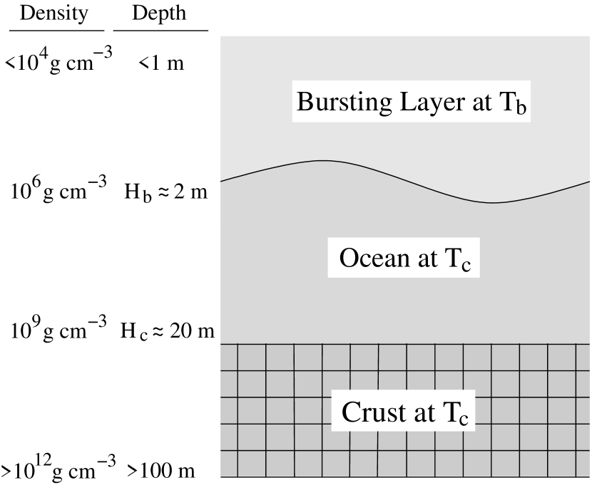
Figure 1.— Diagram of the NS surface layers during the decaying tail of an X-ray burst. The surface is composed of three regions, a hot layer of recently burned fuel with temperature $T_{b}$, a cooler ocean with temperature $T_{c}$, and the outer crust also with $T_{c}$. The bursting-layer/ocean interface is at a depth determined by where unstable burning ignites during the X-ray burst, while the ocean/crust interface occurs at the crystallization depth of the ocean material. Each interface provides a buoyancy that is a natural place for supporting modes. During the beginning of the burst the region just above the bursting-layer/ocean interface is convective, but we ignore this complication to simplify our analysis.

We solve these difficulties by including both the shallow surface wave and the crustal interface wave (Piro & Bildsten, 2005, hereafter PB05). The latter is concentrated in the ocean and rides the ocean/crust interface. These two modes have frequencies close enough that they undergo an avoided crossing during the burst cooling. The case we focus on here is one in which the energy in the surface wave “adiabatically” changes into the crustal interface wave as the burst cools. This switch solves the two problems listed above because: (1) switching to a crustal interface wave ceases the frequency evolution so that the predicted frequency drifts match the observed drifts, and (2) the final frequency is stable and characteristic to each object because it only depends on the crust’s properties, which do not change from burst to burst.

1.2. Outline of Paper

In §2 we use simple analytic arguments to describe our idea for how the surface wave and crustal interface wave interact to reproduce the main features of burst oscillations. In §3 we present time dependent numerical models to simulate the NS surface during the cooling following an X-ray burst. This model is used in §4 to calculate the eigenfrequency spectrum, focusing on the surface wave and crustal interface wave, including rotational modifications expected for a quickly rotating NS. We also estimate the time dependent oscillation amplitude, showing that it decreases as the surface wave changes into a crustal interface wave. In §5 we compare the observed drifts and persistent luminosities with our analytic mode estimates. We consider other modes in §6, and examine the prospects for their detection. We then conclude with a summary of our results in §7.

2. Analytic Summary and Dependence on the Neutron Star Crust

We now outline why the shallow surface wave and crustal interface wave are consistent with the properties of burst oscillations. This demonstrates which properties of the NS crust are constrained by burst oscillation observations.

A shallow surface wave in the hot bursting layer (see Figure 1) has a frequency

$$\omega^{2}_{\rm s}=gH_{b}k^{2}\frac{\Delta\rho}{\rho},$$ (2)

where $g=GM/R^{2}$ is the surface gravitational acceleration, $H_{b}=P/(\rho g)$ is the pressure scale height at the base of the bursting layer, $k^{2}=\lambda/R^{2}$ is the transverse wavenumber, $\Delta\rho/\rho=1-T_{c}\mu_{b}/(T_{b}\mu_{c})$ is the fractional density contrast at the burning depth, and $\mu_{b}$ ($\mu_{c}$) is the mean molecular weight in the bursting layer (ocean). Throughout we assume that the ocean and crust have the same temperature and composition. In the non-rotating limit $\lambda=l(l+1)$, where $l$ is the normal spherical harmonic quantum number. For a quickly spinning NS, $\lambda$ is a function of $\Omega$ and $\omega$, which can be accurately calculated using the “traditional approximation” (as we summarize in §4.2, or see BUC96). In agreement with Heyl (2004) we show that the only low order, rotationally modified angular mode that reproduces all of the properties of the burst oscillations is a buoyant r-mode, which has $\lambda\approx 1/9\approx 0.11$ in the quickly spinning limit (this mode is often identified as the $l=2$, $m=1$ r-mode from the slowly rotating limit, Piro & Bildsten, 2004). Using the scalings from equation (2),

$$\frac{\omega_{s}}{2\pi}=10.8\ {\rm Hz}\left(\frac{2Z_{b}}{A_{b}}\right)^{1/2}\left(\frac{T_{b}}{10^{9}\ {\rm K}}\right)^{1/2}\left(\frac{10\ {\rm km}}{R}\right)$$

$$\times\left(\frac{\lambda}{0.11}\right)^{1/2}\left(1-\frac{T_{c}}{T_{b}}\frac{\mu_{b}}{\mu_{c}}\right)^{1/2},$$ (3)

where $A_{b}$ and $Z_{b}$ are the mass number and charge of the ions in the bursting layer, respectively, and we use an ideal gas equation of state. The final term from the density discontinuity is $\approx 0.8$ near the burst peak. This frequency is consistent with the low-order modes found by McDermott & Taam (1987), but with $\lambda=2$, as appropriate for the $l=1$ modes on a non-spinning NS that they studied.

The crustal interface wave has a frequency set by the cool NS ocean (PB05),

$$\omega^{2}_{c}=\mu_{0}gH_{c}k^{2},$$ (4)

where $\mu_{0}=\mu/P\sim 10^{-2}$ (see §4.1) is the ratio of the shear modulus to the pressure at the top of the crust, and the scale height, $H_{c}$, is evaluated at this same depth. Equation (4) is the dispersion relation for a shallow surface wave, but with a factor of $\mu_{0}$ due to crust compression. For the temperatures expected at the bottom of the ocean, and using a pressure dominated by degenerate, relativistic electrons (PB05)

$$\frac{\omega_{c}}{2\pi}=4.3\ {\rm Hz}\left(\frac{64}{A_{c}}\right)^{1/2}\left(\frac{T_{c}}{3\times 10^{8}\ {\rm K}}\right)^{1/2}$$

$$\times\left(\frac{10\ {\rm km}}{R}\right)\left(\frac{\lambda}{0.11}\right)^{1/2},$$ (5)

where the prefactor is set to match our numerical results, and $A_{c}$ is the mass number of nuclei in the crust.

The shallow surface mode’s frequency decreases as the layer cools. Once $T_{b}$ cools to $T_{c}\approx 3\times 10^{8}\ {\rm K}$ (and using $\mu_{b}/\mu_{c}\approx 1.0$), we find that the surface wave’s frequency drifts by $\approx 9\ {\rm Hz}$, much larger than the observed shifts. This is one of the key problems with explaining the burst oscillations with only a shallow surface wave. When the crustal interface wave is included, it is possible that during the cooling $\omega_{s}=\omega_{c}$, at which point the surface wave evolves into a crustal interface wave (a transition we discuss in §4.3). The frequency then remains fixed because $T_{c}$ does not change during the X-ray burst. The drift then is only $\Delta\omega=\omega_{s}-\omega_{c}$, where $\omega_{s}$ is its value at the beginning of the burst when $T_{b}\approx 10^{9}\ {\rm K}$, resulting in $\Delta\omega/(2\pi)\lesssim 5\ {\rm Hz}$, much closer to observations. In this picture, the size of the drift is approximately set by the composition and temperature of the crust. A crust that is hotter or composed of lighter elements has a higher crustal interface wave frequency, and therefore its drifts are smaller. The observed drifts require a crust with $T_{c}=(2-6)\times 10^{8}\ {\rm K}$ for $A_{c}=50-100$. We come back to these scalings when we consider the observed drifts in §5.

3. Cooling X-ray Burst Envelope Models

We numerically calculate the time evolution of the cooling surface layers and ocean following Cumming & Macbeth (2004). Since the NS radius, $R\approx 10\textrm{ km}$, is much greater than the pressure scale height $H_{c}\approx(2-4)\times 10^{4}\textrm{ cm}$, we approximate the surface as having a constant gravitational acceleration, $g=GM/R^{2}\approx 2\times 10^{14}\textrm{ cm s}^{-2}(M/1.4M_{\odot})(10\ {\rm km}/R)^{2}$ (neglecting general relativity), and plane-parallel geometry. We use $z$ and $x$ as our radial and transverse coordinates, respectively, and in addition find it useful to use the column depth, denoted as $y$ (defined by $dy=-\rho dz$), giving a pressure $P=gy$.

The initial profile of the envelope following the burning is that of a hot, flux dominated, bursting layer sitting above a cooler, lower flux ocean. To mimic this situation, we assume a constant flux of $F_{b}\approx 10^{25}\textrm{ erg cm}^{-2}\textrm{ s}^{-1}$ (basically an Eddington flux as seen in radius expansion bursts that often proceed burst oscillations) above a burning depth column of $y_{b}=3\times 10^{8}\textrm{ g cm}^{-2}$ (Bildsten, 1998). The choice of this depth mainly affects the cooling timescale, with a deeper $y_{b}$ resulting in an extended light curve. This has a small effect on the frequencies since for an electron scattering dominated, constant flux envelope $T_{b}\propto y_{b}^{1/4}$, so from equation (3), $\omega_{s}\propto y_{b}^{1/8}$. Previous studies of constantly accreting NSs have shown that the interior thermal balance is set by electron captures, neutron emissions, and pycnonuclear reaction in the inner crust (Miralda-Escudé, Paczyński, & Haensel, 1990; Zdunik et al., 1992; Bildsten & Brown, 1997; Brown & Bildsten, 1998; Brown, 2000, 2004) which release $\approx 1\textrm{ MeV}/m_{p}\approx 10^{18}\textrm{ erg g}^{-1}$ (Haensel & Zdunik, 1990, 2003). Depending on the accretion rate and thermal structure of the crust, this energy will either be conducted into the core or released into the ocean such that for an Eddington accretion rate up to $\approx 92\%$ of the energy is lost to the core and exits as neutrinos (Brown, 2000). Since we wish to investigate how the properties of the crust affect the characteristics of the burst oscillations we treat this crustal flux, $F_{c}$ as a free variable, and consider its effects around a value of $10^{21}\ {\rm erg\ cm^{-2}}\ {\rm s^{-1}}$ (as expected for $\dot{M}\approx 10^{-9}M_{\odot}\textrm{ yr}^{-1}$, about one-tenth the Eddington rate).

We use the results of Schatz et al. (2001) and Woosley et al. (2004) to set the compositions. Table 2 lists the key properties of our models, which sample a range of conditions expected for the surfaces of bursting NSs. We consider only one nuclear species per layer, where that species is chosen to represent the wide range of elements that actually exist. In He-rich bursts, the burning predominantly produces $\alpha$-elements and cooling lasts $\sim 10\ {\rm s}$ as observed with burst oscillations. We expect more mixing during these bursts due to convection at the ignition depth (Woosley et al., 2004; Weinberg & Bildsten, 2005), so that $\mu_{b}/\mu_{c}\sim 1$. Models 1 and 2 are meant to represent this type of burst, with Model 2 exploring the changes that occur for a large $T_{c}$. On the other hand, bursts with a composition closer to solar (mixed H/He bursts) produce a heavy ocean of ashes from rp-process burning and also less mixing so that $\mu_{b}/\mu_{c}\lesssim 1$. These bursts occur on objects such as GS $1826-24$ (Galloway et al., 2004) and have never shown burst oscillations. Model 3 represents this case, but without the extra heat source of the rp-process burning. This only changes the timescale of the cooling and frequency evolution, and does not affect the calculated mode frequencies nor drifts.

The density of the liquid/solid transition, $\rho_{c}$, when crystallization begins is set by the dimensionless parameter

$$\Gamma \equiv \frac{(Z_{c}e)^{2}}{a_{c}k_{\rm B}T_{c}}$$ (6)

$$= 169\left(\frac{3}{T_{c,8}}\right)\left(\frac{Z_{c}}{30}\right)^{2}\left(\frac{64}{A_{c}}\right)^{1/3}\left(\frac{\rho}{10^{9}\textrm{ g cm}^{-3}}\right)^{1/3},$$

where $k_{\rm B}$ is Boltzmann’s constant, $T_{c,8}\equiv T_{c}/10^{8}\ {\rm K}$, $Z_{c}$ is the charge of the crust nuclei, and $a_{c}=(3/4\pi n_{i,c})^{1/3}$ is the average ion spacing with $n_{i,c}$ the ion number density in the crust. This transition occurs at $\Gamma\approx 173$ (Farouki & Hamaguchi 1993 and references therein), implying a density at the top of the crust,

$$\rho_{c} = 1.1\times 10^{9}\textrm{ g cm}^{-3}\left(\frac{T_{c,8}}{3}\right)^{3}$$ (7)

$$\times\left(\frac{A_{c}}{64}\right)\left(\frac{30}{Z_{c}}\right)^{6}\left(\frac{\Gamma}{173}\right)^{3}.$$

Since material in the crust is simply ocean material that was advected there by accretion, we assume that the ocean and crust have the same composition.

We next construct our envelope models using the parameters summarized above and follow their evolution forward in time. Cooling is described by the heat diffusion equation with no source terms,

$$c_{p}\frac{\partial T}{\partial t}=\frac{\partial F}{\partial y},$$ (8)

where $c_{p}$ is the heat capacity at constant pressure, and the radiative flux is

$$F=\frac{4acT^{3}}{3\kappa}\frac{\partial T}{\partial y},$$ (9)

where $a$ is the radiation constant and $\kappa$ is the opacity. The opacity is set using electron-scattering (Paczyński, 1983), free-free (Clayton 1993 with the Gaunt factor of Schatz et al. 1999), and conductive opacities (Schatz et al. 1999 using the basic form of Yakovlev & Urpin 1980), and we assume that the crust opacity is set in the same way. We solve for $\rho$ using the analytic equation of state from Paczyński (1983). The initial temperature profile is found by integrating equation (9) with the flux profile described above. The envelope is then evolved in time according to equation (8) using finite differencing techniques. We use a grid that is uniform in $\sinh^{-1}[\log(y/y_{\rm b})]$ (Cumming & Macbeth, 2004), so as to properly resolve the temperature jump at the burning depth. Figure 2 shows the initial profile along with the profiles at time steps from $0.1-10.0\ {\rm s}$ for Model 1. The majority of the evolution is concentrated in the outer hot bursting layer with a negligible thermal wave diffusing into the ocean and crust, due to the long thermal time at these depths (consistent with the work of Woosley et al., 2004). These general features are shared by all of the models we consider.

Figure 2.— Temperature, density, and flux for a He-rich bursting NS envelope (Model 1). The initial profile is a flux of $10^{25}\textrm{ erg s}^{-1}\textrm{ cm}^{-2}$ above a column of $3\times 10^{8}\textrm{ g cm}^{-2}$, with a flux of $10^{21}\textrm{ erg s}^{-1}\textrm{ cm}^{-2}$ below (thick solid lines). The curves show time steps of $0.1\ {\rm s}$ (solid), $0.3\ {\rm s}$ (dotted), $1.0\ {\rm s}$ (short-dashed), $3.0\ {\rm s}$ (long-dashed), and $10.0\ {\rm s}$ (dot-dashed). The majority of the time dependent change occurs in the outer hot bursting layer where the local thermal time is short. These profiles extend down into the crust (which begins at a column of $5.3\times 10^{12}\textrm{ g cm}^{-2}$), but here we just focus on the region where the main changes occur.

4. Nonradial Modes During X-ray Burst Cooling

We now calculate the time dependent spectrum of mode frequencies, focusing on the surface and the crustal interface waves. Even though the NS is spinning quickly, $\Omega/(2\pi)\approx 270-620\ {\rm Hz}$, the buoyancy of the envelope dominates over Coriolis effects and determines the radial structure of the modes (BUC96). This is because $N^{2}\sim 10^{10}\ {\rm s^{-2}}\gg R\Omega\omega/H_{c}\sim 10^{6}\ {\rm s^{-2}}$, where the internal buoyancy of the envelope is measured by the Brunt-Väisälä frequency

$$N^{2}=-g\left(\frac{d\log\rho}{dz}-\frac{1}{\Gamma_{1}}\frac{d\log P}{dz}\right),$$ (10)

and $\Gamma_{1}\equiv(\partial\log P/\partial\log\rho)_{s}$ is the adiabatic exponent. Furthermore, since the modes are squeezed into a thin outer layer of thickness $\approx H_{c}\ll R$, they have predominantly transverse amplitudes. Together these properties justify accounting for the effects of rotation by using the “traditional approximation” (BUC96). This simplification allows the angular part of the perturbation equations to be separated from the radial part, and solved as an eigenvalue equation for $\lambda$ (the “effective wavenumber”), where $\lambda$ is a function of $\Omega$ and $\omega$. For this reason, we focus on the radial equations first, and then introduce the angular and spin dependent parts afterwards in §4.2.

4.1. Radial Mode Equations

Solving for the radial eigenfunctions requires considering the governing mode equations both in the bursting layer and ocean, and also in the NS crust. The bursting layer and ocean have no shear modulus, so adiabatic perturbations in this region are described by the nonradial oscillations equations for an inviscid fluid in hydrostatic balance and plane-parallel geometry (Bildsten & Cutler, 1995, hereafter BC95)

$$\frac{d\xi_{z}}{dz}-\frac{\xi_{z}}{\Gamma_{1}H}=\left(\frac{gHk^{2}}{\omega^{2}}-\frac{1}{\Gamma_{1}}\right)\frac{\delta P}{P},$$ (11)

$$\frac{d}{dz}\frac{\delta P}{P}-\left(1-\frac{1}{\Gamma_{1}}\right)\frac{1}{H}\frac{\delta P}{P}=\left(\frac{\omega^{2}}{g}-\frac{N^{2}}{g}\right)\frac{\xi_{z}}{H},$$ (12)

where $\xi_{z}$ is radial displacement and $\delta P/P$ is the Eulerian pressure perturbations. The Eulerian perturbations are related to the Lagrangian perturbations by $\Delta P=\delta P-\xi_{z}\rho g$. When calculating g-modes (including the shallow surface wave), equations (11) and (12) are sufficient since these modes are excluded from the NS crust (BC95). The only exception is the crustal interface mode (PB05), where it is crucial to solve the mode equations with a nonzero shear modulus, $\mu$, in the NS crust (BC95). For a classical one-component plasma the shear modulus is (Strohmayer et al., 1991)

$$\mu=\frac{0.1194}{1+0.595(173/\Gamma)^{2}}\frac{n_{i,c}(Z_{c}e)^{2}}{a_{c}},$$ (13)

where $\Gamma$ is given by equation (6). Since the pressure in the crust is dominated by degenerate, relativistic electrons we rewrite $\mu$ as

$$\frac{\mu}{P}=\frac{1.4\times 10^{-2}}{1+0.595(173/\Gamma)^{2}}\left(\frac{Z_{c}}{30}\right)^{2/3}.$$ (14)

In the crust $\mu/P$ is fairly independent of temperature (except for a small dependence in the factor of $\Gamma$ in the denominator), so we substitute $\mu_{0}\equiv\mu/P$ and assume that $\mu_{0}$ is constant with depth (PB05).

4.2. Rotational Effects

Before the mode equations can be integrated, we must consistently set $\lambda$ with respect to $\omega$ and $\Omega$. The dispersion relation that relates these three variables is described by BUC96 (from the work of Longuet-Higgins 1968), and results in a large variety of angular eigenfunctions for a given radial structure. Heyl (2004) showed that very few of these (just the $m=1$ buoyant r-modes) match the properties of burst oscillations. We summarize these results here, both for completeness and because we consider the presence of additional modes in §6.

Maniopoulou & Andersson (2004) have extended the traditional approximation to include general relativity, which introduces corrections to the co-rotating mode frequencies, $\omega$, due to frame-dragging and red-shifting. Each of these effects contribute differently depending on the angular eigenfunction under consideration, and combined they can decrease $\omega$ by as much as 20%. Since the buoyant r-modes have frequencies independent of spin (as we describe below), we expect frame-dragging to be negligible and red-shifting to be the main change to the normalization of $\omega$ (as is found for the Kelvin mode by Maniopoulou & Andersson, 2004). From equations (3) and (5) we see that such corrections are degenerate with slight changes in the radius and temperature of the NS, and therefore we do not include them.

There are two sets of solutions for $\lambda$, which are both typically presented in the literature as a function of the “spin parameter,” $q=2\Omega/\omega$ (so that for a quickly spinning star $q\gg 1$) The first set is comprised of the rotationally modified g-modes (those with $m\neq-l$) and the Kelvin modes ($m=-l$), which are shown in Figure 3. In the slowly rotating limit, $q\ll 1$, we find $\lambda\approx l(l+1)\approx 2$ or $6$ (for $l=1$ or $2$, respectively), but as the spin increases $\lambda$ splits depending on its $m$ value. It then asymptotes to scaling as $\lambda\propto q^{2}$ (in the case of the rotationally modified g-modes) or as $\lambda=m^{2}$ (in the case of the Kelvin modes).

We present these solutions to emphasize that none of these modes are consistent with burst oscillations. The rotationally modified g-modes all have $\lambda\gg 1$ when the star is rotating quickly. This implies large mode frequencies (see eqs. [3] and [5]), and frequency drifts larger than observed. (In §6 we explore whether these modes exist in burst cooling light curves, but are not seen because of their large frequency drifts.) The Kelvin modes are inconsistent because they are all prograde ($m<0$), so that as the surface cools an observer would see a decreasing frequency.

Figure 3.— Effective wavenumber $\lambda$ as a function of the spin parameter $q=2\Omega/\omega$ for the rotationally modified g-modes ($m\neq-l$) and Kelvin modes ($m=-l$). Solid lines denote modes for which $l=1$ in the non-rotating limit with $m=-1$, $0$, and $1$ (from bottom to top). The dashed lines denote modes for which $l=2$ in the nonrotating limit with $m=-2$, $-1$, $0$, $1$, and $2$ (from bottom to top). For $q\gg 1$, $\lambda\propto q^{2}$, except if $m=-l$, which asymptotes to $\lambda=m^{2}$ (the Kelvin modes). Unfortunately, none of these dispersion relations are consistent with the burst oscillations because they either have frequency shifts much too large (in the case of the rotationally modified g-modes) or shifts with the wrong sign (in the case of the Kelvin modes).

The other set of solutions are a group of modes unique to the case of a rotating star, the r-modes, which we plot in Figure 4. These occur as zero frequency solutions for a non-rotating star, corresponding to incompressible toroidal displacements on the stellar surface. When the star is rotating, Coriolis effects turn these solutions into normal modes of oscillation. In the slowly rotating limit the NS spin and mode frequency are directly proportional,

$$\omega_{r}=\frac{2m\Omega}{l(l+1)},$$ (15)

(Saio, 1982; Lee & Saio, 1986), which are the well-studied inertial r-modes. More relevant for our work here is the case when $q\gg 1$, which are the buoyant r-modes. For $q\gg 1$ the r-modes with $m=l$ exhibit $\lambda\propto q^{2}$, similar to the rotationally modified g-modes from Figure 3, and thus also give frequency shifts too large for burst oscillations. More promising are the r-modes with $m<l$, which have $\lambda\lesssim 1$ and therefore small frequency shifts. Furthermore, since all r-modes have $m>0$, they are traveling retrograde with respect to the NS spin, and provide increasing shifts as the NS cools. We favor the $l=2$, $m=1$ mode (denoted with a thick line in Figure 4) over any of the other $\lambda\ll 1$ r-modes because: (1) $m=1$ is implied from the observations and this is the lowest order $m=1$ mode that gives frequencies and shifts consistent with burst oscillations and (2) any higher order $\lambda\ll 1$ r-mode has multiple bands of hot and cold regions at different latitudes, so that it should be more difficult to observe than the $l=2$, $m=1$ mode. It is rather remarkable that with the number of rotationally modified modes that exist, this is the only one that fits all the required properties! For this mode $\lambda\approx 1/9\approx 0.11$ in the quickly rotating limit, as we used when estimating the mode frequencies in §2.

Figure 4.— Effective wavenumber $\lambda$ as a function of the spin parameter $q=2\Omega/\omega$ for the r-modes. Solid lines denote modes for which $m=1$, with values of $l$ (identified in the slowly rotating limit using eq. [15]) of $1$, $2$, and $3$ (from left to right). Dashed lines denote modes for which $m=2$, with $l=1$, $2$, and $3$ (from left to right). We favor the $l=2$, $m=1$ mode (thick line) as explaining the burst oscillations, which has $\lambda\approx 1/9\approx 0.11$ in the quickly rotating limit.

A further reason for favoring the buoyant r-modes is that their latitudinal eigenfunctions may be easier to observe (Heyl, 2004). Modes with $\lambda\gg 1$ have their eigenfunction squeezed near the equator within an angle $\cos\theta<1/q$, where $\theta$ is measured from the pole. On the other hand, the $m<l$ r-modes and Kelvin modes have much wider eigenfunctions that span most of the surface. This means that given a fixed equatorial perturbation, the pulsed fraction is larger for these latter modes.

4.3. Eigenfunctions and Frequencies in Rotating Frame

Normal modes of oscillation are found by assuming $\Delta P=0$ at the top boundary, which is set at a depth where the local thermal time is equal to the mode period ($t_{\rm th}=2\pi/\omega$, where $t_{\rm th}\equiv c_{p}yT/F$). This top condition, though not unique, is fairly robust since little mode energy resides in the low density upper altitudes (BC95). This is especially true for the two modes we study here, which have their energy concentrated at their respective interface. We numerically integrate the mode equations, shooting for the condition that $\xi_{z}\approx\xi_{x}\approx 0$ deep within the crust, where $\xi_{x}$ is the transverse displacement. This may not be the case in a more realistic calculation of the crust, but as long as we set this bottom depth deep enough, $\approx 10^{17}\ {\rm g\ cm^{-2}}$, we recover the asymptotic solutions of PB05. When we change from integrating the non-viscous mode equations to those appropriate in the crust, we must properly set boundary conditions (PB05).

Figure 5.— Displacement eigenfunctions (given in cm) and energy density (measured in ergs and given by eq. [16]) of the first three low frequency solutions. These are from Model 1 after $0.1\ {\rm seconds}$ of cooling and all with $\lambda=0.11$. The frequencies are in the rotating frame on the NS surface, $\omega$. From high to low frequency (left to right), these are the shallow surface wave, the crustal interface wave, and the first g-mode. All lower frequency solutions are also g-modes. Each lower frequency mode contains an additional node, which are shown by the cusps because we plot the absolute value of the displacements. The transverse displacement, $\xi_{x}$, always has a node at the crust at a column of $5.3\times 10^{12}\ {\rm g\ cm^{-2}}$.

When solving the mode equations we use an effective wave number $\lambda\approx 0.11$, as described in §4.2. There are many solutions to the mode equations, which form a complete basis set of functions. We focus on the low frequency solutions (as opposed to the f-mode or p-modes) because they are a better match to the observed frequencies. These solutions are ordered from high to low frequency, with each successive mode having an additional node in its radial eigenfunctions. In Figure 5 we plot the radial and transverse displacement eigenfunctions ($\xi_{z}$ and $\xi_{x}$, respectively, given in cm) for the first three low frequency solutions from Model 1 after $0.1\ {\rm s}$ of cooling. In addition we plot the energy per logarithm column density,

$$\frac{dE}{d\log y}=\frac{1}{2}4\pi R^{2}\omega^{2}\xi^{2}y,$$ (16)

where $\xi^{2}=|\xi_{x}|^{2}+|\xi_{z}|^{2}$ is the total displacement. This indicates where the kinetic energy of the mode is concentrated. We normalize the total integrated energy of each mode to be $5\times 10^{36}\ {\rm ergs}$, $10^{-3}$ of the total energy released by unstable nuclear burning (Bildsten, 1998). At $9.14\ {\rm Hz}$ (where this is the frequency in the rotating frame on the NS surface, $\omega$) we find a mode with a single node in its eigenfunctions (shown as a cusp in $\xi_{z}$ and less apparent in $\xi_{x}$ because there is always a node at the crust at a column of $y_{c}=5.3\times 10^{12}\ {\rm g\ cm^{-2}}$). Since the energy is concentrated in the bursting layer this is identified as the shallow surface wave. The next mode at $4.30\ {\rm Hz}$ has an additional node and therefore a different parity than the surface wave. Its energy is distributed very differently, largely concentrated at the bottom of the ocean, so it is identified as the crustal interface mode. All modes with lower frequencies are g-modes, and we show the first g-mode (at $3.10\ {\rm Hz}$) with three nodes. These modes are trapped in either the bursting layer or ocean and are identified by a relatively constant energy distribution in each region (the example shown is the prior case).

Since both the surface wave and the first g-mode are concentrated in the bursting layer, they each exhibit frequency drifts as the bursting layer cools, making them both attractive as being burst oscillations. We therefore consider the radiative damping time for each mode to narrow down the choice of radial eigenfunction. The rate of energy loss averaged over one oscillation cycle from an adiabatic perturbation is estimated from the “work integral” (Cox, 1980; Unno et al., 1989), which, when there is no energy source, is

$$\frac{dE}{dt}=\frac{\omega}{2\pi}\oint dt\int\frac{\Gamma_{3}-1}{\Gamma_{1}}\frac{\Delta P}{P}\Delta\left(\frac{dF}{dy}\right)4\pi R^{2}dy,$$ (17)

where $\Gamma_{3}-1\equiv(\partial\log T/\partial\log\rho)_{s}$. The integral is negative when a mode is damped and positive when a mode is excited. From this and the total mode energy (integrating eq. [16]) we can estimate the damping $e$-folding time of a mode’s amplitude,

$$t_{\rm damp}=\left(\int\frac{dE}{d\log y}d\log y\right)\left|\frac{dE}{dt}\right|^{-1},$$ (18)

where the absolute value has been included to make this timescale positive (since all modes we consider are damped).

Figure 6 shows $t_{\rm damp}$ for both the surface wave and the first g-mode as functions of time since the burst peak. To accurately calculate the integral from equation (17) we must drop derivatives of $\Delta P/P$ near the surface because our imposed boundary condition of $\Delta P=0$ results in unphysical local mode excitation (for a description of another way to set this boundary condition see Goldreich & Wu, 1999). The g-mode is damped on a timescale an order of magnitude faster than the surface wave. Though both the first g-mode and the surface wave have energies concentrated in the bursting layer (see far left and right panels at the bottom of Figure 5), each mode’s energy distribution is different within this region. Radiative damping predominantly takes place at the top of the atmosphere (Piro & Bildsten, 2004), so that a mode with more of its energy distributed there is more damped. It is somewhat difficult to see because of the large dynamic range we show, but the energy of the g-mode is approximately constant in the bursting layer, while the shallow surface wave’s energy varies by almost an order of magnitude in the bursting layer (compare the bottom panels on the far left and right of Figure 5). The ratio of damping timescales is therefore approximately the ratio of energies between the top and bottom of the bursting layer. After $\approx 0.5\ {\rm s}$ the g-mode has a damping time shorter than the time for the burst to cool, so that the amplitude of this mode is exponentially damped. Higher-order g-modes have different damping times depending on where they are trapped. Those trapped in the bursting layer (like the example shown) all have similar, short damping times. The g-modes that are trapped in the ocean have much longer damping times ($t_{\rm damp}\approx 5-10\ {\rm s}$), but suffer from very small surface amplitudes. The crustal wave has an even longer damping time ($t_{\rm damp}\gtrsim 10^{3}\ {\rm s}$), but also has the problem of a small surface amplitude. We therefore favor the surface wave as the radial eigenfunction for the burst oscillations because of its combined attributes of having a long damping time coupled with a large surface amplitude from a small input of energy.

Figure 6.— Damping time, $t_{\rm damp}$, as a function of the time since the burst peak, for the mode with a single node (which is initially a surface wave) and the mode with three nodes (the first g-mode), both from Model 1. The dashed line shows were the damping time is equal to the time since burst peak. After only $\approx 0.5\ {\rm s}$ the g-mode is exponentially damped on a timescale shorter than $0.5\ {\rm s}$, so that it will not be observable.

We next consider how the mode frequencies evolve with time since burst peak. In Figure 7 we plot the first two eigenfrequencies as a function of time for Model 1. The mode parity does not change along each continuous line, with one node present for the upper line and two nodes for the lower line. Initially the upper frequency is the surface wave and the lower is the crustal interface wave, consistent with equations (3) and (5). The surface wave’s frequency decreases as the bursting layer cools, eventually running into the crustal mode. This creates an avoided crossing between the two modes (which we highlight in the inset panel of Figure 7). The eigenfunctions therefore change considerably along each line from being characteristic of a surface wave to a crustal interface wave (and vice versa). As long as the evolution of the envelope is sufficiently slow, once excited a mode will most likely evolve along one of these branches and not be able to skip to the other because of differences in parity. We do not show this rigorously, but think this is a reasonable conclusion by considering analogies with perturbation theory problems in non-relativistic quantum mechanics. In cases where the background changes quickly, on a timescale shorter than $\sim 2\pi/\omega$, mixing is highly possible as determined by taking inner products between initial and final states on either side of the avoided crossing. On the other hand, in the case we consider here the background changes very slowly, as is supported by the fact that $d(1/\omega)/dt\lesssim 10^{-2}\ll 1$ (which we calculated to check our conclusions). This implies that the change can be treated as adiabatic, and the modes are not expected to mix at the crossing.

Figure 7.— The frequency evolution of the surface wave and crustal interface wave using Model 1. The upper curve follows the mode with one node in its eigenfunctions, while the lower curve follows the mode with two. The qualitative shapes of the eigenfunctions vary considerably along each curve. Initially, the higher frequency mode corresponds to a shallow surface wave, while the lower frequency mode is a crustal interface wave. As the lines move to the right toward later times, the surface wave is sensitive to the cooling surface layers and decreases, while the crustal wave does not evolve. Eventually the two modes meet at an avoided crossing, which we display in an inset panel. Past the avoided crossing, although the parity has not changed, the higher frequency mode is now like a crustal wave, while the low frequency mode is a surface wave.

In Figure 8 we plot the energy of the single-node wave for a sample of time steps from Model 1. We normalize the total integrated energy of each mode to be $5\times 10^{36}\ {\rm ergs}$. Initially, at $4.0\ {\rm s}$, the mode’s energy is concentrated in the recently burned portion of the upper envelope. As time progresses the energy goes deeper into the star, so that by $12.0\ {\rm s}$, when the burst is nearly over, the energy is concentrated at the bottom of the ocean, just as expected for a crustal mode.

Figure 8.— Energy of the single-node mode per unit logarithmic pressure at different time steps, from Model 1. Each mode is normalized to a total energy of $5\times 10^{36}\ {\rm ergs}$, $10^{-3}$ of the total energy released in an X-ray burst. At early times the mode looks like a shallow surface wave, with its energy concentrated near in the bursting layer, but as it passes through the avoided crossing (see Figure 7) its energy moves continually deeper and becomes more like a crustal interface wave. The sharp feature at a column of $3\times 10^{8}\ {\rm g\ cm^{-2}}$ is due to the density discontinuity at the burning depth. Below a column of $5.3\times 10^{12}\ {\rm g\ cm^{-2}}$ the crust begins and the mode’s energy drops off quickly.

4.4. Observed Frequencies

We now focus on the evolving mode with a single node because it is initially a surface wave, which as discussed in §4.3 is the mode most least likely to be damped and also have an appreciable amplitude. In Figure 9 we use equation (1) to plot the frequencies seen by an inertial observer (solid lines) for a NS spinning at $400\ {\rm Hz}$ (dotted line) for each of our three models. We also show the light curves with a dashed line. In the top panel we plot the results from Model 1. This shows that the NS spin is $\approx 4\ {\rm Hz}$ above the burst oscillation, just the frequency of the crustal mode. In the next two panels we plot the frequency evolution of our other two models, along with their respective light curves. In Model 2, the flux coming through the crust is a factor of 3 higher, providing a significantly hotter crust. This causes the crystallization to happen at much larger depths, resulting in a larger crustal wave frequency. The mode crossing therefore happens earlier, which can be seen by the smaller frequency drift, as expected from the analytic considerations in §2. In Model 3, there is a slightly larger discontinuity at the burning depth due to the heavy ashes from rp-process burning as expected in H/He mixed bursts. This makes the evolution of the surface wave much slower, so that in this case it does not transition into a crustal interface wave, even after $14\ {\rm seconds}$ of cooling. This shows that an avoided mode crossing is not a robust property exhibited by every model. Observations of burst oscillations from such a NS would show more variance in its asymptotic frequency because of this feature. On the other hand, since Model 3 represents an rp-process burst and such bursts do not exhibit burst oscillations, this has not been observed. It is not clear from our models why the He models that show mode crossings are the ones observed, while our H/He models that don’t show crossings are not, especially since frequency drifts like that shown in the bottom panel would be observable if they existed. We discuss these issues further when we conclude in §7.

Figure 9.— The observed frequency evolution of the single-node mode on Models 1, 2, and 3 (solid curves). We use a NS spin of $400\ {\rm Hz}$ (dotted line). For Model 1, this shows that while the mode is a surface wave it evolves upward in frequency, but once it becomes a crustal wave it is very stable at a frequency of $\omega_{c}/(2\pi)\approx 4\ {\rm Hz}$ below the NS spin. In Model 2 the frequency shift ends very early and is only $\approx 3\ {\rm Hz}$ because the crust is much hotter due to a larger crustal flux. On the other hand, in Model 3 we find that an avoided crossing between the surface wave and crustal wave does not occur while the luminosity is at an observable level, so that the frequency never becomes flat. Observations of a NS with oscillations like this would show more variance in their asymptotic frequency in comparison to the other models we consider. The dashed line is the surface luminosity as a function of time, assuming a radius of $10\ {\rm km}$.

As noted by Heyl (2004), since $\lambda\approx 0.11$ as long as $q\gtrsim 10$, any spin NS will exhibit similar frequency evolution as long as $\Omega/(2\pi)\gtrsim 5\omega_{s}/(2\pi)\approx 50\ {\rm Hz}$. This makes it easy to compare models with different spins, and constrains the explanation of burst oscillations as modes since it requires that the frequency shifts be spin independent. This is counter to the studies of Cumming & Bildsten (2000), which predict that the spin and drift size should be correlated. Although EXO $0748-676$ is near this critical frequency (see Table 1), its drift (assuming that it is not yet a crustal interface wave) is still not heavily affected. We find a $\approx 4\ {\rm Hz}$ drift instead of a $5\ {\rm Hz}$ drift at higher rotation rates, so we still predict a spin frequency of $\approx 49\ {\rm Hz}$ for this object.

4.5. Surface Amplitude Evolution

As the surface wave evolves into a crustal wave, we expect the surface amplitude to decrease dramatically since the crustal wave’s energy is mostly at the bottom of the ocean. We estimate $\delta P/P$ at our “surface” where the modes are no longer adiabatic, $t_{\rm th}=2\pi/\omega$, denoted $(\delta P/P)_{s}$, which provides a general idea for how the amplitude is changing. BC95 show that the Eulerian perturbation $\delta P/P$ is constant in the non-adiabatic region, so that we only need to calculate it at our top boundary to estimate its value at the photosphere. Approximately $5\times 10^{39}\ {\rm ergs}$ of energy is released in an X-ray burst, so we assume some small fraction of this is able to power the mode. Since we do not know how much energy actually leaks into the mode, we simply study values which result in reasonably sized perturbations. A key conclusion is that only a small fraction of the available energy is needed, $\sim 10^{-3}$, to get perturbations of order unity. We assume that this energy is conserved throughout the evolution of the mode, an approximation that is justified because the damping time of the mode is always longer than the time that the burst has been cooling.

Figure 10.— Evolution of the surface pressure perturbation for the single-node mode from each of our models. In each case we assume a certain fraction of the X-ray burst’s $5\times 10^{39}\ {\rm ergs}$ of energy has gone into the modes, and is then conserved in the mode as the envelope cools. The fractions we use are $10^{-3}$ (model 1; solid line), $4\times 10^{-3}$ (model 2; dashed line), and $2\times 10^{-4}$ (model 3; dotted line). This demonstrates that appreciable amplitudes can be expected, even if only a small fraction of the burst’s energy goes into the modes. This also highlights how the amplitude quickly dies off once the shallow surface wave turns into a crustal interface mode.

In Figure 10 we plot the surface perturbation as a function of time for all three models. In both Models 1 and 2 the perturbation drops off dramatically once the surface wave turns into a crustal interface wave, especially in the case of Model 2, which has a thicker ocean. If the top of the crust is too deep the resulting surface amplitude will be too small to explain burst oscillations. The total displacement is about constant down to the crust with $\xi\approx\xi_{x}\approx\xi_{z}R/h$ since the modes are nearly incompressible. From our top boundary condition of $\Delta P=0$ we find $(\xi_{z}/h)_{s}=(\delta P/P)_{s}$, so that together $\xi\sim(\delta P/P)_{s}R$. Using the scalings from equation (16), along with the crustal mode frequency from equation (5) and the density of crystallization from equation (7), the total crustal wave energy at late times is approximately

$$E_{{\rm total},c}\sim 5\times 10^{36}\ {\rm ergs}\left(\frac{64}{A_{c}}\right)\left(\frac{30}{Z_{c}}\right)^{20/3}\left(\frac{R}{10\ {\rm km}}\right)^{2}$$

$$\times\left(\frac{\lambda}{0.11}\right)\left[\frac{(\delta P/P)_{s}}{0.1}\right]^{2}\left(\frac{T_{c}}{3\times 10^{8}\ {\rm K}}\right)^{5},$$ (19)

where the prefactor has been set to match the numerical results. The predominant effect is that the surface amplitude is very sensitive to the depth of the crust so that $(\delta P/P)_{s}\propto Z_{c}^{20/3}T_{c}^{-5/2}$ for fixed energy. In Model 3 the switch to a crustal interface wave never occurs, so that the amplitude always stays large. An interesting feature of all the models is that at early times the amplitude actually increases. This is because as the frequency initially decreases the displacements must increase to maintain the same energy. Suggestively, the time evolutions of the amplitudes, especially for Model 1, are similar to the amplitudes measured by Muno, Özel, & Chakrabarty (2002).

4.6. Magnetic Field Limits

The lack of persistent pulsations from the non-pulsar burst oscillation sources implies a smaller magnetic field for these objects. To prevent channeled accretion the surface dipole field must be less than (Frank, King, & Raine, 1992)

$$B_{\rm acc}=5.1\times 10^{7}\ {\rm G}\left(\frac{M}{1.4M_{\odot}}\right)^{1/4}\left(\frac{10\ {\rm km}}{R}\right)^{5/4}$$

$$\times\left(\frac{\dot{M}}{10^{-9}\ M_{\odot}\ {\rm yr^{-1}}}\right)^{1/2}.$$ (20)

Both the shallow surface wave and the crustal interface wave exhibit large shears in their transverse displacements. Following BC95, the maximum magnetic field before the waves would be dynamically affected is $B^{2}\approx 8\pi H^{2}\rho\omega^{2}$, where $H$ is chosen as appropriate for each mode. For the surface wave this gives a limit (using eq. [3]),

$$B_{s}=8.8\times 10^{7}\ {\rm G}\left(\frac{2Z_{b}}{A_{b}}\frac{T_{b}}{10^{9}\ {\rm K}}\right)\left(\frac{y_{b}}{3\times 10^{8}\ {\rm g\ cm^{-2}}}\right)^{1/2}$$

$$\times\left(\frac{1.4M_{\odot}}{M}\frac{\lambda}{0.11}\right)^{1/2}\left(1-\frac{T_{c}}{T_{b}}\frac{\mu_{b}}{\mu_{c}}\right)^{1/2}.\hskip 14.22636pt,$$ (21)

surprisingly close to $B_{\rm acc}$ considering that these two limits result from vastly different physical mechanisms. For the crustal interface mode (using eqs. [5] and [7]),

$$B_{c}=1.2\times 10^{10}\ {\rm G}\left(\frac{64}{A_{c}}\right)\left(\frac{30}{Z_{c}}\right)^{11/3}\left(\frac{T_{c,8}}{3}\right)^{3}$$

$$\times\left(\frac{1.4M_{\odot}}{M}\frac{R}{10\ {\rm km}}\right)\left(\frac{\lambda}{0.11}\right)^{1/2},$$ (22)

where we assume $\Gamma=173$. This is much higher than either of the two previous limits because the crustal interface wave “lives” at such high pressures. The lack of persistent pulses from the majority of X-ray bursters is likely because of a weak field in the bursting layer and ocean (Cumming, Zweibel, & Bildsten, 2001), making our non-magnetic mode calculation adequate for now.

5. Comparisons with Observed Drifts

Brown, Bildsten, & Rutledge (1998) showed that the core of a transiently accreting NS reaches a steady-state set by nuclear reactions deep in the crust, so that the luminosity departing the crust is given by the time-averaged accretion rate (Brown, 2000). This means that crustal temperatures can be inferred from an observable property, namely the average persistent luminosity. Given the discussion from §2, we expect objects with small observed drifts to have larger persistent luminosities.

Figure 11.— The frequency drifts, $\Delta\omega/(2\pi)$, as a function of the persistent luminosity, $L_{\rm pers}$ (in units of $L_{\rm Edd}=2.5\times 10^{38}\ {\rm erg\ s^{-1}}$). Two different crustal models are plotted (Brown 2005, private communication) with compositions of ⁵⁶Fe (thick solid line) and ¹⁰⁶Pd (thick dashed line). We assume that $A_{b}/Z_{b}=2$, $\mu_{b}/\mu_{c}=1.0$, and that initially $T_{b}=10^{9}\ {\rm K}$. We compare this with the largest observed frequency drifts of the non-pulsar, bursting NSs (see Table 1). The observed drifts should be viewed as lower limits since observational or excitation-related effects may result in the initially observed surface wave having $T_{b}<10^{9}\ {\rm K}$. The horizontal bars indicate the range of luminosities shown by each object, with a point at the average luminosity. Open circles indicate NSs that show radius expansion bursts at the same time as burst oscillations, while solid triangles indicate NSs that do not. 4U $1728-34$, Aql $X-1$, and 4U $1636-536$ have shown both cases.

In Figure 11 we plot predicted frequency drifts using the difference of equations (3) and (5). We relate $T_{c}$ to the persistent luminosity, $L_{\rm pers}$, using the crustal models of Brown (2005, private communication) for compositions of ⁵⁶Fe (thick solid line) and ¹⁰⁶Pd (thick dashed line). These models are based on the calculational techniques described in Brown (2004). We then plot the observed luminosities and largest observed frequency drifts from Table 1. The total range of observed luminosities is shown by the horizontal bars with a point placed at the average luminosity. Open circles indicate objects for which burst oscillations are coincident with radius expansion bursts, while solid triangles indicate those that are not. We use an Eddington luminosity of $L_{\rm Edd}=2.5\times 10^{38}\ {\rm erg\ s^{-1}}$ so as to be consistent with the work of Ford et al. (2000). The observed drifts should be viewed as lower limits since the surface wave may not be excited until the bursting layer’s temperature is below the $T_{b}=10^{9}\ {\rm K}$ that we use here. Qualitatively, the higher luminosity NSs show smaller drifts, as expected from our models. Furthermore, lighter crustal material is favored for explaining the observations. This is consistent with the cooling timescale of the bursts (see Table 1), which suggest He-rich bursts that produce iron-like nuclei ( and would not produce rp-process elements such as ¹⁰⁶Pd). In general, these objects are not all expected to have the same crustal composition, and this can be studied by making further comparisons with detailed modeling and consideration of each system’s bursting and binary properties.

6. Could Other Angular Modes be Present?

Figure 12.— Frequency evolution of the lowest angular-order, rotationally modified modes from Model 1. All modes are $l=1$, unless otherwise noted, where $l$ refers to the latitudinal quantum number in the slowly spinning limit. In every case the radial structure is the single-node mode as we focus on for the burst oscillation. The mode frequencies are denoted by solid lines, with the NS spin as a dashed line. In (a) we consider a spin of $300\ {\rm Hz}$ and find that its frequency shifts are somewhat smaller than for a $600\ {\rm Hz}$ spin as shown in (b). Even so, all the frequency shifts are much larger than the $l=2$, $m=1$ r-mode that we favor as the burst oscillations (which is also plotted for comparison; thick solid line).

In §4.2 we considered the multitude of rotationally modified solutions available, all with the same single node radial structure, and identified only one that satisfied the properties of burst oscillations. The other low angular-order modes resulted in frequency shifts that were too large, and sometimes in the wrong direction. Nevertheless, these modes may be compelling to study since a priori we do not have a reason to exclude them, and more sensitive observations may reveal these additional modes. Such a measurement of multiple modes would revolutionize our knowledge of an accreting NS’s mass, radius, spin, and surface layers.

We calculate the time dependent frequencies from Model 1, this time considering a variety of the low angular-order modes, all with the same single-node radial eigenfunction as used for the burst oscillation. We compare NS spins of both $300\ {\rm Hz}$ (Fig. 12a) and $600\ {\rm Hz}$ (Fig. 12b) (dashed lines). Generally, a faster spin shows larger frequency drifts for these modes because $\lambda\propto q^{2}$. This is not the case for the $l=2$, $m=1$ r-mode we favor as the burst oscillation, which shows no dependence on $\Omega$ (thick solid lines). When the cooling is fastest at early times, the frequency shifts are dramatic, ranging anywhere from $\approx 15\ {\rm Hz}$ (for the Kelvin modes) to $\approx 100\ {\rm Hz}$ (for the rotationally modified g-modes). Such large shifts have not been seen in previous frequency searches of X-ray burst lightcurves, but may be lurking, undetected. On the other hand, because of the late time frequency stability afforded by the crustal mode, one could argue that if these modes existed they would have already been detected when the frequency evolution is weak. The resolution of this question depends on the actual oscillation amplitude. If the burst oscillations are any indication, the amplitudes are largest soon after the burst peak when the frequency shift is greatest. The stable part of the frequency might then have an amplitude below detectable levels. It remains an important exercise to search the extensive database of burst lightcurves for signatures of oscillations similar to what we describe here.

7. Conclusions and Discussion

We considered nonradial surface oscillations as a possible explanation for the oscillations observed during type I X-ray bursts on non-pulsar accreting NSs. In studying the time evolution of a shallow surface wave, we found that this mode changes into a crustal interface wave as the surface cools, a new and previously unexplored result. This phenomenon allows us to match both the observed frequency shifts and the high stability of the asymptotic frequency of burst oscillations. To find frequencies in the observed range, the modes must be highly modified by rotation, resulting in the NS spin occurring merely $\approx 4\ {\rm Hz}$ above the burst oscillation frequency. Following similar reasoning to Heyl (2004), we find that the majority of the rotationally modified modes cannot match all of the observed properties of burst oscillations, because they predict too large of drifts and/or drifts of the wrong direction. The $l=2$, $m=1$ buoyant r-mode ($\lambda\approx 0.11$) overcomes all of these difficulties, and for this reason it is the favored mode to explain the burst oscillations. Perhaps not coincidentally, this mode has other attractive qualities such as a wide latitudinal eigenfunction that may make it easier to observe.

An important mystery that we did not resolve here is why burst oscillations in the non-pulsars are only seen in the short $\sim 2-10\ {\rm s}$ bursts (not counting the superbursts), a decay timescale indicative of He-rich fuel at ignition. While Models 1 and 2 show frequency and amplitude evolution similar to what has been observed for burst oscillations, Model 3 does not. This is not unexpected because the first two (especially Model 1) reflect what we expect for He-rich bursts, but it is at the same time perplexing because we have no reason a priori to explain why burst oscillations as from Model 3 are not observed. There must then be some physical mechanism for why they are not seen. In the study by Cumming & Bildsten (2000), they find that modulations in the flux at the burning depth can be washed out if the thermal time is too long in the hydrostatically expanding and contracting surface layers. This effect is dependent on the mean molecular weight so that it is weak for He-rich bursts, but fairly strong for mixed H/He bursts. It is possible that a similar phenomena occurs just above the nonradial modes that we study here.

There remain many properties of burst oscillations that are not studied in our work here (for example, see the observations of Muno, Özel, & Chakrabarty, 2002, 2003). The characteristics of the oscillating light curves, the energy dependence of the pulsed amplitudes, and the phase shifts of different energy components all can be used to learn about the accreting NSs that are exhibiting these burst oscillations. Such investigations have just been initiated by Heyl (2005) and Lee & Strohmayer (2005).

The most exciting implication of our study is that the asymptotic frequencies and drifts are directly related to properties of the surface NS layers. The crustal interface wave depends on the attributes of the crust, which in turn is a product of the X-ray burst properties, and especially its superburst properties. Superbursts are deep enough to directly impact the composition of the NS ocean, and eventually, as material advects down with the accretion flow, the crust. The accreting low mass X-ray binary 4U $1636-536$ has exhibited oscillations during a superburst (Strohmayer & Markwardt, 2002), and during X-ray bursts both before and after (Zhang et al. 1997; M. Muno 2004, private communication), all with the same asymptotic frequency. Energetically, superbursts could easily excite crustal waves since they are roughly a thousand times more energetic than normal X-ray bursts. For the frequency to be the same in each occurrence the crustal properties could not have changed during this time. This is possible as long as 4U $1636-53$’s superburst recurrence time is short enough that the crust keeps a steady state composition. A crust at $\approx 10^{13}\ {\rm g\ cm^{-2}}$ requires $\approx 7\ {\rm yrs}$ at an accretion rate of $10^{-8}\ M_{\odot}\ {\rm yr^{-1}}$ to be replaced by new, accreted material. Such a timescale favors a crust that has not changed significantly given that 4U $1636-53$ has produced three superbursts in the last $4.7\ {\rm yrs}$ (Wijnands, 2001; Strohmayer & Markwardt, 2002; Kuulkers et al., 2004).

Note added in proof.—It has been brought to our attention by Dong Lai that our arguments in §4.3 for adiabatic evolution through the avoided crossing may not be correct. We currently use the condition that adiabatic evolution occurs as long as the mode frequency is much larger than the cooling rate. If the avoided crossing instead acts analogously to neutrino oscillations (J. Bahcall 1989, Neutrino Astrophysics [Cambridge: Cambridge Univ. Press]) or photon propagation on magnetized neutron stars (D. Lai & W. C. G. Ho 2002, ApJ, 566, 373) the correct comparison would be the frequency difference at the avoided crossing versus the cooling rate. If this is indeed the case, then the surface mode will not solely couple to the crustal interface mode. Instead, some energy would remain in the surface mode as the frequencies cross. We are currently studying this problem.

Table 1Properties of X-ray Burst Oscillations from Non-pulsars

	$\omega/(2\pi)$	$\Delta\omega/(2\pi)$	$\tau$	Radius	$L_{\rm pers}/L_{\rm edd}$	References
Object	(Hz)	(Hz)	(s)	Expansion?	(%)
EXO $0748-676$	45	. . .	. . .	No	$0.9-3.6$	1,2
4U $1916-053$	270	$3.58\pm 0.41$	. . .	No	$1.3-5.6$	3,4
4U $1702-429$	330	$1.6-3.0$	$1.9-4.0$	No	$3-6$	5,6,7,8
					$1.1-8$	9
4U $1728-34$	363	$2.1-3.75$	$1.8-6.2$	Yes and No	$3.3-9.8$	2,6,7,10,11
					$2-7$	8
SAX J$1748.9-2021$	410	. . .	13.0	No	. . .	12
KS $1731-260$	524	$0.9-2.0$	$2.6-4.1$	Yes	$25$	7,13,14,8
					$1.2-14.4$	9
Aql X-1 ($1908+005$)	549	$2.4-4.0$	$2.7$	Yes and No	$1-3$	7,15,16,8
4U $1658-298$	567	$\approx 0.5-5$	$6.9-12.5$	Yes	$0.2-1$	7,17,18,19
4U $1636-536$	582	$1.0-3.0$	. . .	Yes and No	$2.2-7.8$	2,7,20,21,22
					$10-15$	8
					$5.6-12.8$	9
Galactic Center Source	589	$\approx 1$	. . .	Yes	. . .	23
SAX J$1750.8-2980$	601	$\approx 3\tablenotemark{f}$	$\approx 3$	Yes	$0.2-4.8$	24,25
4U $1608-522$	619	$\approx 1$	. . .	Yes	$4.4-17.4$	2,7,26
					$0.7-6$	8

References. — (1)Villarreal & Strohmayer (2004); (2) van Paradijs, Penninx, & Lewin (1988); (3) Galloway et al. (2001); (4) Boirin et al. (2000); (5) Markwardt, Strohmayer, & Swank (1999); (6) Strohmayer & Markwardt (1999); (7) Muno et al. (2002); (8) Ford et al. (2000); (9) Cornelisse et al. (2003); (10) Strohmayer et al. (1996); (11) van Straaten et al. (2001); (12) Kaaret et al. (2003); (13) Smith, Morgan, & Bradt (1997); (14) Muno et al. (2000), (15) Zhang et al. (1998); (12) Cumming & Bildsten (2000); (13) Wijnands, Strohmayer, & Franco (2001); (18) Wijnands et al. (2002); (19) Wijnands et al. (2003); (20) Strohmayer et al. (1998); (21) Miller (2000); (22) Strohmayer (1999); (23) Strohmayer et al. (1997); (24) Kaaret et al. (2002); (25) Natalucci et al. (1999); (26) Hartman et al. (2003)

Table 2Cooling Neutron Star Models

Model	Bursting Layer	Ocean/Crust	$F_{c}$ (erg cm-2 s-1)	$\mu_{0}\equiv\mu/P$	$\rho_{c}$ (g cm-3)	$\mu_{b}/\mu_{c}$
1	40Ca	64Zn	$10^{21}$	$8.8\times 10^{-3}$	$1.8\times 10^{9}$	0.94
2	40Ca	64Zn	$3\times 10^{21}$	$8.8\times 10^{-3}$	$9.3\times 10^{9}$	0.94
3	64Zn	104Ru	$10^{21}$	$1.1\times 10^{-2}$	$3.4\times 10^{8}$	0.90

References

- Abramowicz, Kluźniak, & Lasota (2001) Abramowicz, M. A., Kluźniak, W., & Lasota, J. P. 2001, A&A, 374, L16
- Bildsten (1995) Bildsten, L. 1995, ApJ, 438, 852
- Bildsten (1998) Bildsten, L. 1998, in The Many Faces of Neutron Stars, ed. R. Buccheri, J. van Paradijs & A. Alpar (Dordrecht: Kluwer), 419
- Bildsten & Brown (1997) Bildsten, L. & Brown, E. F. 1997, ApJ, 477, 897
- Bildsten & Cutler (1995) Bildsten, L. & Cutler, C. 1995, ApJ, 449, 800 (BC95)
- Bildsten, Ushomirsky, & Cutler (1996) Bildsten, L., Ushomirsky, G. & Cutler, C. 1996, ApJ, 460, 827 (BUC96)
- Boirin et al. (2000) Boirin, L., Barret, D., Olive, J. F., Bloser, P. F., & Grindlay, J. E. 2000, 361, 121
- Brown (2000) Brown, E. F. 2000, ApJ, 536, 915
- Brown (2004) Brown, E. F. 2004, ApJ, 614, L57
- Brown & Bildsten (1998) Brown, E. F. & Bildsten, L. 1998, ApJ, 496, 915