Electric field representation of pulsar intensity spectra

Abstract

Pulsar dynamic spectra exhibit high visibility fringes arising from interference between scattered radio waves. These fringes may be random or highly ordered patterns, depending on the nature of the scattering or refraction. Here we consider the possibility of decomposing pulsar dynamic spectra – which are intensity measurements – into their constituent scattered waves, i.e. electric field components. We describe an iterative method of achieving this decomposition and show how the algorithm performs on data from the pulsar B0834+06. The match between model and observations is good, although not formally acceptable as a representation of the data. Scattered wave components derived in this way are immediately useful for qualitative insights into the scattering geometry. With some further development this approach can be put to a variety of uses, including: imaging the scattering and refracting structures in the interstellar medium; interstellar interferometric imaging of pulsars at very high angular resolution; and mitigating pulse arrival time fluctuations due to interstellar scattering.

1 Introduction

In the last few years there has been much progress made in understanding the interference fringes which are manifest in pulsar dynamic spectra. Representing the data as power spectra (“secondary spectra”) of the dynamic spectra demonstrated the underlying simplicity of the complex organised fringe patterns which are sometimes seen: commonly it is found that the power is concentrated on parabolic loci in the transform domain (Stinebring et al 2001). This property is now understood in the following terms (Stinebring et al 2001; Walker et al 2004; Cordes et al 2005). The dynamic spectrum is the electric field intensity, $I(\nu,t)$, as a function of radio-frequency, $\nu$, and time, $t$; the conjugate (Fourier) variables are the delay, $\tau$, and Doppler-shift, $\omega$, of the scattered waves. The purely geometric component of the delay is proportional to the square of the scattering angle, whereas the Doppler-shift is proportional to one component (the component parallel to the effective transverse velocity vector) of the scattering angle, leading to parabolic relationships between $\tau$ and $\omega$.

The well-defined parabolae which are often seen further require that the scattering material not be distributed along the line-of-sight, but instead must be concentrated into a thin “screen” (Stinebring et al 2001). In some cases the data also suggest that the scattering is highly anisotropic (Walker et al 2004; Cordes et al 2005).

To date the interpretation of observed dynamic/secondary spectra has proceeded by forward theoretical modelling; in other words models are constructed and the predicted secondary spectra are compared with the data. This approach has yielded important insights, but it is fundamentally limited in that a detailed match to the data is not practicable — only the general characteristics can be considered. This is a severe limitation because dynamic spectra may contain a great wealth of detailed information in the $\sim 10^{6}$ independent frequency-time measurements which can be routinely recorded. Consequently we are motivated to attempt inverse modelling of dynamic spectra, whereby the electric fields are deduced by modelling the observed intensity distribution. If the total electric field is $U(\nu,t)$, then $I(\nu,t)=U^{*}(\nu,t)\,U(\nu,t)$, so $|U(\nu,t)|=\sqrt{I(\nu,t)}$ tells us the field amplitudes, but the phases remain a priori unknown. This is an example of a “phase retrieval problem”; such problems are common in the optics literature (e.g. Fienup 1982; Elser 2003; McBride, O’Leary and Allen 2004), although we were unaware of that resource until the present work was largely complete.

This paper presents an iterative approach to solving the inversion problem; it is not the only approach, nor is it necessarily the best approach, but it has been at least partially successful. The outline of the paper is as follows: in the next section we describe the physical model we have adopted and derive the mathematical basis for our inversion algorithm; our attempt at implementing this algorithm is described in §3, while in §4 we show how this implementation performs on real data; possible applications of these techniques are discussed in §5.

2 Foundation of the inversion

As radio-waves propagate through the Galaxy they are subject to refraction and scattering by inhomogeneities in the ionised interstellar medium (e.g. Rickett 1991; Narayan 1992). If the radio-waves originate from a pulsar then the size of the source is small, and the coherent patch correspondingly large, so that essentially all pairs of scattered/refracted waves yield high-visibility interference fringes, regardless of the spatial separation of the scattering centres. Consequently the combination of scattered waves can be well approximated simply by addition of the various electric field components. (We consider departures from this point-like source approximation in §5.3.) Denoting the total electric field as $U(\nu,t)$, and each of the discrete scattered waves as $u_{j}(\nu,t)$, we have

$$U(\nu,t)=\sum_{j}u_{j}(\nu,t)=\sum_{j}\widetilde{u}_{j}\exp\left[2\pi i(\nu\tau_{j}+\omega_{j}t)\right].$$ (1)

Equivalently, we can write this relationship in the Fourier Transform domain, $(\nu,t)\rightarrow(\tau,\omega)$, as

$$\widetilde{U}(\tau,\omega)=\sum_{j}\widetilde{u}_{j}\,\delta(\tau-\tau_{j})\,\delta(\omega-\omega_{j}),$$ (2)

where $\delta$ denotes the Dirac delta-function, and the $\widetilde{u}_{j}$ are complex constants. The intensity observed at radio frequency $\nu$ (relative to band centre) and time $t$ (relative to the central epoch of the observation) is $I(\nu,t)=U^{*}(\nu,t)\,U(\nu,t)$. Given an observed $I(\nu,t)$, we want to determine $U(\nu,t)$. More precisely, because the conjugate variables $(\tau,\omega)$ have clear physical interpretations, as the delay and Doppler-shift of the scattered waves, we wish to determine $\widetilde{U}(\tau,\omega)$. In this model the individual scattered waves which make up $\widetilde{U}$ are completely specified by their delay ($\tau_{j}$), Doppler-shift ($\omega_{j}$), amplitude and phase (the single complex number $\widetilde{u}_{j}$).

We have taken an iterative approach to solving for $\widetilde{U}$, given $I$, as we now describe. Given a model electric field, $U_{0}$, we can compute the corresponding intensity pattern. In general this will not match the data exactly and we want to improve the model. Suppose our model differs from the true electric field by an amount $\delta U_{0}$, we can then write

$$I(\nu,t)=U^{*}U=U_{0}^{*}U_{0}+\delta U_{0}^{*}U_{0}+U_{0}^{*}\delta U_{0}+\delta U_{0}^{*}\delta U_{0}.$$ (3)

(Where there is no ambiguity we will henceforth not make explicit the independent variables.) Introducing the residual between model and data, ${\cal R}_{0}(\nu,t):=I-U_{0}^{*}U_{0}$, we arrive at

$${\cal R}_{0}=\delta U_{0}^{*}U_{0}+U_{0}^{*}\delta U_{0}+\delta U_{0}^{*}\delta U_{0}.$$ (4)

Providing the existing model is a good one $\left(|\delta U_{0}|\ll|U_{0}|\right)$ we can neglect the last term in this expression and estimate the quantity $\delta U_{0}$ from the resulting linear approximation.

Now suppose that $\delta U_{0}$ is dominated by a single scattered wave, so that our task reduces to a determination of the properties of that wave, then we can make the approximation

$$\delta U_{0}(\nu,t)=\delta\widetilde{U}_{0}\exp\left[2\pi i(\nu\tau+\omega t)\right],$$ (5)

for some particular (but unknown) values of $(\tau,\omega)$, where $\delta\widetilde{U}_{0}$ is a complex constant. Dropping the final term in equation 4, multiplying by $U_{0}(\nu,t)\exp\left[-2\pi i(\nu\tau+\omega t)\right]$ and integrating yields

$$\int\!\!{\rm d}t\,{\rm d}\nu\,{\cal R}_{0}U_{0}\exp\left[-2\pi i(\nu\tau+\omega t)\right]=\qquad\qquad\qquad\$$ (6)

$$\ \qquad\qquad\qquad\delta\widetilde{U}_{0}^{*}\!\int\!\!{\rm d}t\,{\rm d}\nu\,U_{0}^{2}\exp\left[-4\pi i(\nu\tau+\omega t)\right]$$ (7)

$$+\;\;\;\delta\widetilde{U}_{0}\!\int\!\!{\rm d}t\,{\rm d}\nu\,U_{0}^{*}U_{0}.$$ (8)

Although the first two terms on the right-hand side of equation 4 are comparable in magnitude, their counterparts in equation 6 are not; generally the term in $\delta\widetilde{U}_{0}$ is expected to dominate the term in $\delta\widetilde{U}_{0}^{*}$, because only a small subset of the power in $U_{0}$ contributes to the coefficient in $\delta\widetilde{U}_{0}^{*}$, whereas (by Parseval’s theorem) all of the power in $U_{0}$ contributes to the coefficient of $\delta\widetilde{U}_{0}$. Noting that $\int\!{\rm d}t\,{\rm d}\nu\,U_{0}^{*}U_{0}\simeq\int\!{\rm d}t\,{\rm d}\nu\,I(\nu,t)$, because $|\delta U_{0}|\ll|U_{0}|$, we see that we can choose $\int\!{\rm d}t\,{\rm d}\nu\,U_{0}^{*}U_{0}=1$ at the outset, by appropriately normalising the dynamic spectrum. Neglecting the conjugate image (i.e. the term in $\delta\widetilde{U}_{0}^{*}$) then leads to the simple form

$$\delta\widetilde{U}_{0}=\widetilde{{\cal R}_{0}U_{0}}.$$ (9)

This result gives us an estimate for the (complex) amplitude of the scattered wave which is missing from the model, as a function of the assumed delay and Doppler-shift of that wave. This result has been derived under the assumption that $\delta U_{0}$ is dominated by a single scattered wave, so that the appropriate choices of delay and Doppler-shift are those values for which the modulus of the right-hand-side attains its largest value.

The result just derived shows how, given a model electric field $U_{0}$, we can improve that model by adding a single scattered wave component. Moreover the process can clearly be iterated, so that the restriction embodied in equation 5 – i.e. that $\delta U_{0}$ can be approximated by a single plane wave – is unimportant: the full spectrum of scattered waves can be built up iteratively. This is done by adding one new component to the reference model, $U_{0}$, on each iteration. In its overall structure this procedure is similar to that of the CLEAN algorithm (Högbom 1974) which is commonly employed in aperture synthesis imaging in radio astronomy; that algorithm inspired the one presented here.

We need to assume a model as a starting point for an iterative solution; in the absence of any specific a priori information about the scattered waves, the most sensible choice is a zero-frequency ($\tau,\omega=0$) plane wave model. This choice may correspond, physically, to an unscattered wave. However, we note that the interference fringe properties depend on delay/Doppler differences, so our model predicts the same dynamic spectrum for the scattered wave field $\widetilde{U}_{1}(\tau,\omega)$ as it does for $\widetilde{U}_{2}(\tau,\omega)=\widetilde{U}_{1}(\tau+\tau_{0},\omega+\omega_{0})$. This point can be recognised most easily if we write down one of the interference terms contributing to $I=U^{*}U$:

$$\widetilde{u}_{k}^{*}\widetilde{u}_{j}\exp[2\pi i\{\nu(\tau_{j}-\tau_{k})+(\omega_{j}-\omega_{k})t\}].$$ (10)

This degeneracy means that there is no information in the dynamic spectrum on the absolute delay and Doppler shift of the scattered waves, just as there is no information on absolute phase ($\widetilde{u}_{k}^{*}\widetilde{u}_{j}=|\widetilde{u}_{k}||\widetilde{u}_{j}|\exp[i(\phi_{j}-\phi_{k})]$), and the origin in our model $\widetilde{U}$ is arbitrary.

2.1 Weak scattering limit

To our knowledge only one previous attempt has been made to derive the scattered wave spectrum from a recorded dynamic spectrum: B.J. Rickett (personal communication 2003) derived a solution $\{\widetilde{u}_{j},\tau_{j},\omega_{j}\}$ in the weak scattering limit. In this limit all of the scattered wave components are of very low amplitude in comparison with the unscattered component, and to obtain a solution all of the cross-terms $\widetilde{u}_{j}^{*}\widetilde{u}_{k}$ with $j,k\neq 0$ are neglected. This approximation has a simple correspondence with the approach we have described. Because the scattered components are all very weak, there is no need to keep refining the model electric field, $U_{0}$, and consequently it is not necessary to iterate the solution: we simply take all of the field components $\delta\widetilde{U}_{0}$ returned by equation 7 for the starting model, $U_{0}=1$. This yields the solution in the weak scattering limit: $\widetilde{U}=\widetilde{U}_{0}+\delta\widetilde{U}_{0}=\widetilde{I}(\tau,\omega)$. Our approach, by contrast, employs an unscattered reference wave ($U_{0}=1$) only for the first cycle of the iteration process; all subsequent cycles differ from the weak scattering limit by including the identified scattered components in the reference model, and in general $U_{0}\neq 1$ in equation 7.

3 An implementation of the algorithm

To evaluate the procedure described in the previous section we first tested it on a simple synthetic dynamic spectrum made up of four scattered wave components plus a small amount of pseudo-random “noise”. Whereas the derivation in §2 makes no particular assumption about the sampling of $I(\nu,t)$, our synthetic dynamic spectrum, and the real data discussed in §4, were sampled on a regular grid in radio-frequency and time. In Fourier space, our representation of these data need only employ wave components with conjugate variables (delay and Doppler-shift) which lie on a uniformly spaced grid satisfying the Nyquist sampling criterion; our algorithm employs such a grid.

We found that the algorithm did indeed locate (in delay-Doppler space) the electric-field components which we knew to be present, but it did not make accurate estimates of the (complex) field amplitudes when the components were first identified. This is not surprising because the procedure described in §2 employs simplifying assumptions, so equation 7 is not expected to give a very accurate estimate of the component amplitudes. This property would be unimportant if subsequent iterations refined the values of the component amplitudes so that the algorithm converged on the correct solution. In fact the procedure generated spurious components, instead of converging on the correct values of the actual field components, thus smearing power around in delay-Doppler space. This behaviour yields results of low dynamic range and is unacceptable.

Because of the poor performance of the procedure described in §2, we decided to refine the algorithm slightly. Instead of simply accepting the largest Fourier coefficient in equation 7 as the appropriate estimate of the wave amplitude, we refined the estimate by adjusting the wave amplitude and phase so as to achieve a least-squares fit of the revised model to the dynamic spectrum. In this scheme the estimate provided by equation 7 is used to fix $\tau$ and $\omega$ for the new component, as before, but the (complex) amplitude indicated by equation 7 is used only as the starting point for the least-squares minimisation. By fitting to the data we sidestep many of the concerns which might otherwise arise in connection with the approximations made in deriving equation 7 — linearisation, the single component approximation, and neglect of the conjugate image. In short the revised procedure should work well providing only that the largest Fourier component of ${\cal R}_{0}U_{0}$ is also the largest Fourier component of the difference between the reference field and the actual field ($\delta U_{0}=U-U_{0}$). We found that this algorithm did indeed perform well, yielding reconstructions which matched the input as closely as possible (i.e. to within the “noise”), and did not generate any spurious components beyond what would be expected given the “noise” level of the “data” — i.e. the algorithm did not limit the dynamic range of the results. In summary, the successful algorithm follows the procedure specified in §2, but at each iteration the amplitude and phase of the new electric field component (identified via equation 7) is determined by least squares fitting to the data. The algorithm is described in detail in the following section.

3.1 Details of the algorithm

The algorithm was implemented in IDL, a high-level, commercial software package which provides straightforward array manipulation and data display. The main elements of the algorithm are:

(i) The data are preconditioned; this involves three steps. First we remove the spectral profile, $B(\nu)$, which is imposed by the bandpass filter; this is part of our routine data reduction process, with $B(\nu)$ determined from a calibration data set. Secondly, the effects of intrinsic fluctuations in the pulsar’s flux are removed, in so far as possible; these fluctuations manifest themselves as a purely temporal modulation, $f(t)$, with a white noise spectrum. We dealt with this modulation by forming the frequency-averaged intensity at each timestep; we then filtered out the high-frequency components in this quantity, by mutiplying by a Gaussian function of full-width-half-maximum equal to one half of the Nyquist frequency, and transformed back to yield a smoothed version of the average intensity; finally we made our estimate of $f(t)$ from the ratio of these two quantities. Correcting the data for the effects of pulse-to-pulse variations is then simply a matter of dividing $I(\nu,t)$ by $f(t)$. It must be acknowledged that this prescription is not ideal, as it does not completely eliminate the intrinsic flux variations, and it also attenuates the wave interference structure slightly. The final step is to normalise to unit mean intensity.

(ii) The starting model for $U_{0}$ is taken to be a wave of unit amplitude and zero phase, with $\tau,\omega=0$.

(iii) A new scattered wave component is then identified as the largest component in equation 7 which has $\tau\geq 0$. Physically we expect that all delays should be non-negative relative to the unscattered wave; the algorithm can in principle differentiate between waves of positive and negative delay, so it should be able to discover this property. However, if the unscattered wave is very strong, so that $\widetilde{U}\simeq\delta(\tau)\,\delta(\omega)$, then $\widetilde{U}_{0}\simeq\widetilde{U}_{0}^{*}$ and it is difficult for any practical scheme to avoid confusion between a scattered wave and its complex conjugate. As the latter are all equivalent to scattered waves which have $\tau\leq 0$, there is potential for choosing spurious components, and in practice we found that this did indeed happen. To avoid this problem we imposed the restriction $\tau\geq 0$ on all components.

Our input data consist of measurements of field intensity on a regular grid in radio-frequency and time – the dynamic spectrum – so for these data the Fourier plane (delay-Doppler) representation requires only components on a regular, Nyquist-sampled grid. Consequently we chose our scattered wave components to lie on a Nyquist-sampled grid in $(\tau,\omega)$.

(iv) The amplitude and phase of the new component are adjusted by minimising the sum of squares of the difference between the model and the data. Minimisation of several component amplitudes/phases is undertaken simultaneously, using the “Amoeba” algorithm described in Numerical Recipes, which is implemented within the IDL software package. The ‘scale’ parameter used by the Amoeba algorithm is initially set to 0.2, when a new component is first introduced, and then is reduced by a factor 0.7 on each subsequent iteration (i.e. every time another component wave is added to the model). Only components whose scale parameters are greater than some value (we employed $2\times 10^{-3}$) are included in our least-squares minimisation; these criteria mean that 13 scattered wave components are routinely included. In addition, because the unscattered wave ($\tau,\omega=0$) is often very strong this component is also included in the optimisation, making 14 wave components in total.

This gradual “freeze-out” of component amplitudes, as the Amoeba scale parameter gradually decreases, was incorporated into our algorithm in order that components with similar amplitudes could be simultaneously adjusted (optimised) in an efficient way. This aspect of the algorithm has an additional benefit: it helps to guard against the possibility of spurious parameter determinations arising from local, rather than global minima found by Amoeba. If Amoeba finds a local minimum, with correspondingly erroneous component amplitudes, on a given iteration, it may well find its way out of the local minimum to reach the global minimum on the next iteration cycle. Only one of the 14 component amplitudes ceases to be adjusted on each cycle, so the algorithm has a fair degree of robustness to the potential problems caused by local minima in the chi-squared hyper-surface. If, for some reason, the algorithm were to fix a component amplitude at a value which is badly in error, then that error may be fixed in later iteration cycles, as there is no barrier to putting new components in the same place as existing components if that is where the largest difference between model and data occurs.

(v) We used the reduced chi-squared value (chi-squared per degree of freedom) to measure the success of our model in fitting the data. Each new scattered wave component that is added to the model should lower the reduced chi-squared, if that component is significant; however, once the algorithm reaches the noise level, the new components are (by definition) no longer significant, and the addition of any given component is just as likely to increase the reduced chi-squared as to decrease it. To reflect this change in behaviour we forced the algorithm to terminate when 3 successive iterations (i.e. new scattered wave components) each caused the reduced chi-squared value of the fit to increase. This criterion causes the algorithm to terminate very quickly once the noise level is reached, while remaining robust to the presence of a small number of insignificant components in the solution (i.e. the algorithm is not tripped up by isolated insignificant components). It is possible to check the significance of each wave component in the solution set $\{\widetilde{u}_{j},\tau_{j},\omega_{j}\}$ returned when the algorithm terminates, and then cull insignificant components; this would be a reasonable requirement to enforce, but the fraction of such spurious components is expected to be very small and to date we have not employed any culling.

4 Performance with real data

To be useful, the algorithm must be able to cope with real data. We tested our code on a dynamic spectrum of the pulsar B0834+06, taken at an observing frequency of 321.0 MHz with the Arecibo radio telescope. We used the WAPP backend signal processors to record 1024 channels across a total of 1.563 MHz of bandwidth. We sampled the spectrum every 4.096 ms and formed a pulse-phase-averaged estimate of the on-pulse and off-pulse spectra which we used to calculate the ON - OFF spectrum. We then averaged this over 10 s to form one column in the dynamic spectrum. The results of a 45 minute observation are shown in figure 1 in the form of the measured dynamic spectrum (top left) and secondary spectrum (power spectrum; bottom left), compared with the corresponding values reproduced by our model (right). From these results we can see that the model yields a convincing representation of the data: the deficiencies of the modelling are not apparent to the eye in either the dynamic spectrum or the secondary spectrum representations.

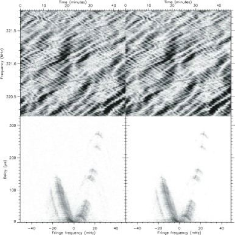
Figure 1: Data (left) and model (right) for an observation of PSR B0834+06, in a 1.563 MHz band centred on 321.00 MHz. The data were taken with the Arecibo radio telescope in conjunction with the WAPP backend signal processing units, on MJD 53009; there are 1024 spectral channels, and 270 time samples, each of 10 seconds duration. The top panels show dynamic spectra, while the lower panels show the corresponding secondary spectra (power spectra of the dynamic spectra). Inverse grey-scale (black is peak intensity) is used in all cases; the transfer function is linear for the dynamic spectra, and logarithmic for the secondary spectra. The signal/noise ratio on each pixel of the observed dynamic spectrum is 2.7, on average, yielding a dynamic range of 63 dB on the corresponding secondary spectrum. The model reproduces the data well.

The model dynamic and secondary spectra shown in figure 1 are of course derived quantities; the model itself is the set of scattered waves (electric field components) represented by $\{\widetilde{u}_{j},\tau_{j},\omega_{j}\}$. In figure 2 we show the scattered wave amplitudes, $|\widetilde{u}(\tau,\omega)|$; the roughly parabolic relationship between $\tau$ and $\omega$ is evident in this plot. These results also show how the scattering/refracting centres are picked out very clearly in this representation of the data as power concentrations in delay-Doppler space. It is beyond the scope of this paper to analyse the information present in the scattered wave solutions, so we will say nothing specific about the meaning of the results shown in figure 2; nor do we plot the phases of the various components. Various applications of our technique are, however, discussed in general terms in §5.

In fact our scattered wave model for these data is not acceptable, in the sense that its chi-square value is too large, given the number of degrees of freedom. There are $1024\times 270$ independent pixels in the dynamic spectrum; in the model there are 8720 scattered waves, each of which is described by four parameters (amplitude, phase, delay and Doppler-shift), and the total over all pixels of the squared-residual between model and data is $2.88\times 10^{5}$, in units of the noise on the dynamic spectrum. This corresponds to a reduced chi-squared value ($\chi^{2}_{r}$, chi-squared per degree of freedom) only slightly larger than unity: $\chi^{2}_{r}=1.19=2.88\times 10^{5}/(1024\times 270-8720\times 4)$; but a statistically acceptable model would have a reduced chi-square value much closer to unity ($|\chi^{2}_{r}-1|\la 0.01$), so although figure 1 is impressive it is possible to do much better. In other words the differences between model and data are not due to noise alone.

A clearer test of the performance of the algorithm comes from differencing the model and observed secondary spectra, as the latter exhibits a very high dynamic range. We find that this difference has a dynamic range of 47 dB, compared to the 63 dB dynamic range of the input data. These figures confirm that the model accounts for the majority of the structure in the data, but the residuals are far from noise-like. We expect that substantial improvements in the quality of the fit would be possible if the 8720 (complex) component amplitudes were simultaneously optimised. Global least-squares optimisation of our solution has not been attempted by us. With such a large number of free parameters, a global optimisation is not an easy task: in a linearised approach the simultaneous equations we are required to solve have $\sim 3\times 10^{8}$ non-zero coefficients.

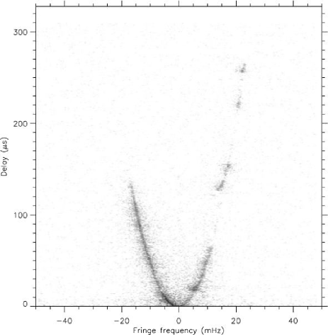
Figure 2: The amplitudes, $|\tilde{u}_{j}|$, of the 8720 scattered wave components identified by the algorithm described in §3, operating on the dynamic spectrum shown in figure 1. These wave components form the basis from which the model dynamic and secondary spectra in figure 1 are derived. The axes are delay ($\tau$), and Doppler shift ($\omega$). In this figure we can see that the individual scattered waves cluster tightly around a parabolic locus with $\tau\propto\omega^{2}$. An inverse logarithmic grey-scale is used for this figure.

5 Discussion

As noted above, the algorithm we have described does not generate a statistically acceptable description of the data shown in figure 1. However, it was not obvious at the outset of this study that the type of spectral decomposition process we sought would work at all, so the partial success we are able to report is in fact quite encouraging. We expect that much better fits to data will be achieved in future with further development of this technique. In part our confidence stems from the fact that a pulsar dynamic spectrum can be expected to be accurately modelled by the form $I(\nu,t)=U^{*}U$ (once calibration etc. is taken care of), and the job is simply to find $U$. More precisely, the job is to find the phase of $U$, since the amplitude is known directly from $I$. This emphasises the importance of a fact mentioned in the introduction: this type of problem, i.e. phase-retrieval, has previously been addressed in various contexts in the optics literature, and future work on dynamic spectrum decomposition should make full use of that resource. Our particular application corresponds to the problem of retrieving a “complex-valued object” (in our case, $\widetilde{U}$) from the modulus of its Fourier transform ($|U|=\sqrt{I}$); this is recognised as a difficult problem (McBride, O’Leary and Allen 2004). An acceptable model should yield noise-like residuals (in both dynamic and secondary spectra), and should satisfy the constraint that the number of free parameters be very much less than the number of independent measurements of the dynamic spectrum. Our current algorithm fails on the first of these criteria. We expect that a globally optimised solution – in which all free parameters are simultaneously adjusted – would come much closer to achieving noise-like residuals, but we have not yet demonstrated this. With such a large number of free parameters, a global optimisation would be computationally challenging.

An important limitation of the algorithm we have presented is that it is restricted to finding scattered waves with $\tau\geq 0$. Under many circumstances this limitation does not cause problems. However, if there are multiple refracted images present then problems can arise. To see why, we need to consider the properties of the starting model: a single component of unit amplitude at $\tau,\omega=0$; what does this component represent? Because the data themselves only carry information about the relative Doppler-shifts, delays and phases amongst the various wave components, the choice of origin is arbitrary. In practice, because the starting model places all of the flux in a single wave, the origin actually corresponds to the component which contains the largest flux. If there is only a single refracted image present, then this component will also be the component with the smallest delay. However, if there are multiple refracted images present, then the brightest of these might well not be the path with the smallest delay. In this circumstance the algorithm will fail to find the scattered and refracted wave components which have smaller delays than the starting model – because they have $\tau<0$ – and cannot be expected to return an accurate model of the electric fields, regardless of how many iterations are performed.

Our description of the received signal in terms of scattered wave components may be used for a variety of purposes; to date we have recognised three main applications, which we describe in the following sections.

5.1 Imaging the ionised ISM

The scattered wave components are identified by the values of their delay and Doppler-shift, $\tau$ and $\omega$. If the scattering occurs in a single, thin screen – as often seems to be the case when organised patterns are seen in a dynamic spectrum (Stinebring et al 2001) – then there is a direct relationship between these coordinates and the apparent positions of the scattering centres. This relationship takes a simple form in cases where the observed delays are dominated by the geometric path delay, leading to parabolic features in the secondary spectrum; this circumstance is quite common (Stinebring et al 2001; Cordes et al 2005). If the mapping between $(\tau,\omega)$ and position can be determined, then the scattered waves can be remapped to give an image of the refracting/scattering centres. Such a picture would be complex (containing both ampltitude and phase information), and detailed, and should provide valuable insights into the ionised component of the interstellar medium. In particular it will be helpful in elucidating the nature of the anomalous scattering and refracting screens which are known to cause a variety of phenomena – Extreme Scattering Events (Fiedler et al 1987, 1994); refraction and multiple imaging in pulsars (e.g. Hewish 1980; Cordes and Wolszczan 1986; Rickett, Lyne and Gupta 1994; Hill et al 2005); and intra-day variability in compact radio quasars (Kedziora-Chudczer et al 1997; Dennett-Thorpe and de Bruyn 2000; Bignall et al 2003). These phenomena are poorly understood (Rickett 1991, 2001).

5.2 Quantifying pulse TOA errors

If some of the signal arriving at the telescope is delayed, then a measurement of the pulse Time-Of-Arrival (TOA) will be affected by this delay. As the scattering geometry necessarily changes from epoch to epoch, this is a source of systematic errors in precision pulsar timing observations. Such studies are important for tests of fundamental physics – the equation of state of matter at nuclear densities, for example – for low-frequency gravitational wave detection, and for precision time-keeping (Foster and Backer 1990). Eliminating propagation errors in pulse TOAs would therefore be valuable. By analysing dynamic spectra with the technique we have presented, we obtain detailed information about the various paths from source to observer, allowing us to quantify the effects of multi-path propagation on the pulse TOAs. In turn this means that we should be able to eliminate this contribution to the systematic errors in TOAs if high resolution dynamic spectra are recorded in tandem with the timing information.

We can envisage two different schemes for correcting the scattering errors in pulse TOAs. The simplest scheme would be to compute the net delay due to all the known paths, and then subtract this delay from the corresponding TOA. The second scheme is much more ambitious: if the pulse TOA is determined from off-line reduction of baseband data, then we can, in principle, process those data in such a way that the electric fields from the various scattered paths are coherently recombined with the unscattered signal. This generalises and extends the concept of coherent de-dispersion (Hankins and Rickett 1975), whereby the “filtering” imposed by propagating the signal through a cold plasma is precisely removed by applying the inverse filter. Coherent de-dispersion is now routinely used to process baseband data on radio pulsars. By analogy with a phase-conjugate mirror, which eliminates wavefront errors by exactly reversing light propagation paths, we can term a coherent recombination of the scattered signal “Virtual Phase Conjugation” (VPC). VPC has the potential to completely remove the signal filtering imposed by (multi-path) interstellar propagation, and thus to eliminate the associated contributions to pulse TOA errors. By the same token, VPC should permit studies of pulsar microstructure (e.g. Hankins 1996) at very high time-resolution.

5.3 High resolution imaging of the source

In §5.1 we noted that the scattered wave decomposition yields, fairly directly, an image of the scattering medium. With some further development it should also permit interferometric imaging of the pulsar itself. To see why, we need only recall how terrestrial radio interferometers operate: the correlation between pairs of signals is evaluated as a function of baseline, i.e. separation between the antennas. A high visibility amplitude for a given source means that the coherent patch is larger than the baseline length, so the source must be small. Conversely, if the visibility amplitude is small then the baseline is longer than the size of the coherent patch, and we have resolved the source on this baseline. Exactly the same considerations apply to the interference between the scattered waves discussed here; in our case the interferometric baseline is simply the transverse separation of the paths at the location of the scattering screen.

In the particular approach we have described in this paper the scattered waves are identified under the assumption of a point-like source (see §2) with an infinitely large coherent patch, so that all pairs of scattered waves, $j,k$ yield fringes of amplitude $|\widetilde{u}_{j}||\widetilde{u}_{k}|$. For very large scattering angles, this approximation must break down, and in this case the data can be used to image the source in a manner directly analogous to terrestrial radio astronomy, namely by quantifying the fringe visibility as a function of baseline length. This technique is fundamentally similar to previous investigations which used interstellar scattering to constrain the size of pulsar radio-emission regions (Gwinn 2001; Gwinn et al 1997; Wolszczan and Cordes 1987). There are two main advantages of the method proposed here. First, it makes use of a lot more information — all the contributing propagation paths are elucidated, thus permitting many more constraints on the model brightness distribution of the pulsar. Secondly, by knowing the geometry of all the contributing paths we can re-order the visibility data into the usual coordinate system (the “$u,v$ plane”) used for radio astronomical imaging with terrestrial interferometers. From that position the many powerful concepts, techniques and tools developed for synthesis imaging can be brought to bear on the problem of imaging via interstellar scattering.

5.4 Interstellar holography

B.J. Rickett (personal communication, 2003) has previously noted the close analogy between his scattered wave solution, derived in the weak scattering limit (§2.1), and Gabor holography. The scattered wave decomposition described in this paper goes beyond the weak scattering approximation, but the relationship to holography remains strong. In both cases the dynamic spectrum can be regarded as an in-line (Gabor) hologram of the interstellar medium. In the weak scattering limit the hologram is recorded with a plane reference wave, in effect – the strong, unscattered wave – and can be reconstructed with such a wave to yield an image of the scattering medium. In this paper we have considered the more general circumstance where the amplitudes of the scattered components are not negligibly small, and their mutual interference must be taken into account. In this case the dynamic spectrum is analogous to a hologram recorded with an aberrated reference wave, and reconstructing an image is no longer so straightforward. Our approach will permit images to be reconstructed computationally for this situation. The connection with Gabor holography is worth bearing in mind because many powerful techniques have been developed in that domain, and some may be useful in interstellar holography.

6 Conclusions

We have considered the possibility of representing pulsar dynamic spectra in terms of an identifiable collection of electric field components whose mutual interference yields the observed intensity structure. Such a representation is of interest because of the direct link between the properties of the field components and the characteristics of the contributing propagation paths through the interstellar medium. An algorithm for achieving this decomposition has been derived, implemented, and tested on high-quality data; it works well, although the resulting model is not formally an acceptable representation of the data as the residuals are not noise-like. Further development of this technique should permit insights into a variety of issues relating to interstellar wave propagation and the physics of pulsars.

7 Acknowledgments

We have benefitted from helpful discussions with several colleagues: Simon Johnston, Barney Rickett, Jim Cordes, Bill Coles, Curtis Asplund, Ben Stappers, Willem van Straten and Leon Koopmans. At the University of Sydney this work was supported by the Australian Reseach Council, at the Kapteyn Institute and ASTRON by the Netherlands Organisation for Scientific Research, and at Oberlin by the National Science Foundation.

References

- (1) Bignall H.E. et al 2003 ApJ 585, 653
- (2) Cordes J.M., Wolszczan A. 1986 ApJL 307, L27
- (3) Cordes J.M. et al 2005 ApJ (Submitted: astro-ph/0407072)
- (4) Dennett-Thorpe J., de Bruyn A.G. 2000 ApJL 529, L65
- (5) Elser V. 2003 J. Opt. Soc. Am. A 20, 40
- (6) Fiedler R.L. et al 1987 Nature 326, 675
- (7) Fiedler R.L. et al 1994 ApJ 430, 581
- (8) Fienup J.R. 1982 Appl. Opt. 21, 2758
- (9) Foster R.S., Backer D.C. 1990 ApJ 361, 300
- (10) Gwinn C.R. 2001 ApSS 278, 65
- (11) Gwinn C.R. et al 1997 ApJL 483, L53
- (12) Hankins T. 1996 ASP Conf. Ser. 105, 197
- (13) Hankins T.H., Rickett B.J. 1975 Meth. Comp. Phys. 14, 55
- (14) Hewish A. 1980 MNRAS 192, 799
- (15) Hill A. et al 2005 ApJL 619, L171
- (16) Högbom J.A. 1974 A&AS 15, 417
- (17) Kedziora-Chudczer L. et al ApJL 490, L9
- (18) McBride W., O’Leary N.L., Allen L.J. 2004 PRL 93, 233902
- (19) Narayan R. 1992 RSPTA 341, 151
- (20) Rickett B.J. 1991 ARAA 28, 561
- (21) Rickett B.J. 2001 ApSS 278, 5
- (22) Rickett, B.J., Lyne A.G., Gupta Y. 1997 MNRAS 287, 739
- (23) Stinebring D.R. et al 2001 ApJL 549, L97
- (24) Walker M.A. et al 2004 MNRAS 354, 43
- (25) Wolszczan A., Cordes J.M. 1987 ApJL 320, L35