FUSE Measurements of Far Ultraviolet Extinction. I. Galactic Sight Lines

Abstract

We present extinction curves that include data down to far ultraviolet wavelengths (FUV; 1050 – 1200 Å) for nine Galactic sight lines. The FUV extinction was measured using data from the Far Ultraviolet Spectroscopic Explorer. The sight lines were chosen for their unusual extinction properties in the infrared through the ultraviolet; that they probe a wide range of dust environments is evidenced by the large spread in their measured ratios of total-to-selective extinction, $R_{V}$ = 2.43 – 3.81. We find that extrapolation of the Fitzpatrick & Massa relationship from the ultraviolet appears to be a good predictor of the FUV extinction behavior. We find that predictions of the FUV extinction based upon the Cardelli, Clayton & Mathis (CCM) dependence on $R_{V}$ give mixed results. For the seven extinction curves well represented by CCM in the infrared through ultraviolet (x $<$ 8 µm^-1), the FUV extinction is well predicted in three sight lines, over-predicted in two sight lines, and under-predicted in 2 sight lines. A Maximum Entropy Method analysis using a simple three component grain model shows that seven of the nine sight lines in the study require a larger fraction of grain materials to be in dust when FUV extinction is included in the models. Most of the added grain material is in the form of small (radii $\lesssim$ 200 Å) grains.

1 Introduction

Little is known about Galactic extinction in the far ultraviolet region of the spectrum (FUV; 912 – 1150 Å or 8.7 - 11.0 $\mu$m^-1; in this paper we include wavenumbers from 3.3 – 8.7 $\mu$m^-1 in what we refer to as the UV since IUE covered this spectral region) other than that it is relatively strong, it increases with increasing wavenumber, and is variable among sight lines. The strength of FUV extinction requires that it be properly considered when recovering the intrinsic spectrum of an object. This is true for most observations taken in the FUV as well as for ultraviolet (UV; 1150 – 3300 Å or 3.3 – 8.7 µm^-1) or optical observations of significantly red-shifted objects. The light extinguished at FUV wavelengths plays a major role in the energetics of star-forming galaxies since a large fraction of energy in starlight is processed to long wavelengths through absorption and re-emission by dust. Molecular cloud physics and chemistry are also greatly affected by the amount of UV and FUV radiation that penetrates such regions; it is these wavelengths that will most affect the formation and destruction of molecules. Finally, the strength and variation of FUV extinction make it a valuable diagnostic for better characterizing the mass of material in and the compositions of small grains ($\lesssim 200$ Å).

Extinction curves in the ultraviolet (3.3 – 8.7 $\mu$m^-1) have been well approximated by two empirical relationships. For the first of these, Fitzpatrick & Massa (1986; 1988; 1990, hereafter FM) found an expression for extinction that relies on six parameters, two that account for an underlying linear extinction ($c_{1}$ and $c_{2}$), three that describe the strength, location, and width of the 2175 Å bump ($c_{3}$, $x_{0}$ and $\gamma$) and one that describes the curvature of the rise toward the FUV ($c_{4}$). These parameters are simply coefficients in mathematical functions that were fit to UV data, and have no known physical basis. Fitzpatrick (1999) argues that the location of the 2175 Å  bump is stable and that the underlying linear extinction can be varied with a single parameter, so that FM fits can be well determined with only four parameters. The consistent position of the 2175 Å feature is confirmed by Valencic et al. (2004) who find no shifted bumps in a sample of over 400 Galactic sight lines. However, in this paper we will use the traditional six-parameter FM fits.

In a different empirical analysis, Cardelli, Clayton & Mathis (1988; 1989, hereafter CCM) used data from the infrared to the UV to find an average relationship for extinction as a function of wavenumber that relies on a single parameter, the ratio of total-to-selective extinction, $R_{V}$ = A_V/E(B-V). $R_{V}$ values are interpreted as being related to the grain environment since they correlate with particle size in dust grain models. The CCM relationship seems to be appropriate for the vast majority ($\sim 99\%$) of Galactic sight lines with known extinction curves (Valencic et al., 2004) indicating that extinction from the infrared (IR) to UV varies in a systematic way among a wide range of dust environments. A potential value of the CCM formulation is its general predictive capabilities, providing an extinction curve from the IR through UV (0.3 – 8.7 $\mu$m^-1) based only on photometric observations at IR and optical wavelengths.

The first measurements of extinction beyond 8.7 $\mu$m^-1 (below 1150 Å) were made with Copernicus. From these initial few sight lines: $\zeta$ Oph, $\xi$ Per, $\alpha$ Cam and $\sigma$ Sco (York et al., 1973; Snow & York, 1975) it became evident that the FUV curves are generally a continuation of the UV extinction trend, and that the extinction continues to rise out to 10 $\mu$m^-1. CCM made a tentative extension of their extinction relation beyond 8 $\mu$m^-1 using the Copernicus data. Although the extrapolation was based only on a few sight lines, the congruence of these extinction curves demonstrated that the average $R_{V}$-dependent law extends beyond 8 $\mu$m^-1 in the Galaxy. In addition, CCM showed that a simple extension of the FM fit to FUV wavelengths gives, on average, a fair representation of the actual extinction in this spectral region. The Savage & Mathis (1979) “average” interstellar extinction curve beyond 9 $\mu$m^-1 is based entirely on Copernicus observations of three sight lines. In the nearly thirty years since Copernicus, a few additional reddened sight lines in the Galaxy have been measured in the FUV using Voyager, HUT, ORFEUS, FUSE and suborbital rockets (Longo et al., 1989; Snow, Allen & Polidan, 1990; Green et al., 1992; Buss et al., 1994; Hutchings & Giasson, 2001; Sasseen et al., 2002; Lewis, Cook & Chakrabarti, 2005). The extinction curves produced in these papers are broadly consistent with extrapolations of the FM and CCM relationships into the FUV.

Though the cited studies revealed some evidence that extinction curves continue to rise beyond 8.7 $\mu$m^-1, the paucity of appropriate data did not allow for a systematic study of FUV extinction, including a rigorous determination of whether an extrapolation of FM or CCM to FUV wavelengths would be appropriate in a diverse set of interstellar environments. Instrumental issues of scattered light, time-variable sensitivity, and a limited sample of target and comparison stars have limited the utility of the Copernicus data set (Jenkins, Savage, & Spitzer, 1986; Snow, Allen & Polidan, 1990). The Voyager UVS data also suffer from low resolution which prevents explicit characterization and removal of the effects of molecular hydrogen absorption. Hopkins Ultraviolet Telescope and ORFEUS have produced insufficient data for a systematic survey, and rocket-borne instruments have not probed diverse regions (Lewis, Cook & Chakrabarti, 2005). FUSE is the first instrument that has produced an appropriate data set for undertaking a thorough and careful analysis of FUV extinction over a wide range of sight line conditions.

This is the first in a series of three papers that will explore extinction in the FUV. Paper II in the series (Cartledge et al., 2005) will present our first results for FUV extinction in the Magellanic Clouds. Paper III (in preparation) will employ a much larger sample of sight lines ($\gtrsim$ 70) in order to provide a greater statistical significance to trends in observed extinction properties. The present study investigates FUV extinction characteristics in nine Galactic sight lines that span a wide range of dust environments as measured by $R_{V}$ (a proxy for dust grain properties). We explore how the extinction curves from 8.7 – 9.5 $\mu$m^-1 (1150 - 1050 Å) relate to extrapolations from the FM and CCM relationships. We also apply a simple model to the extinction curves in order to investigate how the addition of FUV data might change the constraints on dust characteristics. Though our 3-component grain model does not account for the full complexity of dust in the interstellar medium, the model results do provide a rough guide for estimating mass requirements among the grain components. In §2 we present the observations, data reduction procedures, and modeling algorithm. We discuss the nature of the sight lines, analyze the extinction curves in terms of FM and CCM fits, and consider model implications for the “small grain” population in §3. A summary is given in §4.

2 Observations, Data Reduction and Analysis

2.1 Far Ultraviolet Spectra

The FUV data used for this study were obtained with FUSE through the low-resolution (LWRS) aperture resulting in a resolution on the order of R = 20,000 and covering a wavelength range from approximately 950 to 1185 Å(or 10.5 – 8.4 $\mu$m^-1). The observations, originally obtained for a variety of programs (including our own), were made between October 1999 and September 2001. The basic characteristics of the observations including the FUSE target designations, the observing modes, and the exposure times are summarized in Table 1. The data were retrieved from the FUSE archive and recalibrated using CALFUSE version 2.2.1. We found that calibrations with versions of CALFUSE earlier than 2.0 did not possess sufficient photometric accuracy for determining reliable extinction curves, for instance see Hutchings & Giasson (2001). The eight calibrated spectra for each data set were mapped to a common wavelength array spanning the entire range of the data. The data were merged by finding the mean flux at each wavelength point, weighted by three broad signal-to-noise bins determined for each individual spectrum. The error arrays were merged in a manner consistent with that of the data arrays. For several observations, there were obvious misalignments of the star in the aperture, resulting in low or absent flux values for individual spectra. Such bad data segments were flagged before merging the spectra and were given zero weight in the co-addition. The FUSE data anomaly known as the “worm” (Sahnow, 2003) was also present in a majority of the observations. The flux values that were lowered by this anomaly were also flagged, and thus did not contribute to the final merged spectra. Merged spectra were co-added in the case of multiple observations of an individual sight line.

For our sample of stars, we note that the flux values in the wavelength overlap region between the IUE and FUSE data (1150 – 1185 Å) match well. This contrasts with the lower signal-to-noise Magellanic Cloud sight line data of Cartledge et al. (2005) who, in some cases, needed to scale their FUSE data in order to provide a better match to the IUE flux levels.

2.2 Corrections for H₂ and H i

Absorption features produced by interstellar molecular hydrogen can have a substantial effect on the observed FUV spectrum of a star. That is to say, a considerable fraction of the light below $\sim$1108 Å may be absorbed by this molecule. Although the strongest lines of each H₂ band can reduce the observed flux to nearly zero, the broad overlapping damping wings are able to be modeled and removed (i.e., the spectrum is rectified to the true continuum level). In addition, the numerous narrow lines due to rotationally excited states can be reliably removed, with the exception of strongest line cores. Even some of the lightly reddened stars (some of our comparison stars) can show enough H₂ absorption that we chose to remove it. Our techniques for measuring the column densities of each rotational state are described by Rachford et al. (2001, 2002). In brief, we use profile fitting to measure the strongest lines, and a curve of growth analysis for the weaker lines. The latter analysis also gives an “effective” $b$-value for the rotationally excited lines, which is necessary because we generally do not have velocity structure information for H₂. We generate a model transmission spectrum based on the retrieved column densities and $b$-value. Because slight wavelength mismatches will result in a poor removal of the H₂ spectrum, we perform a running cross-correlation between the model and the observed spectrum. This produces a map of the appropriate wavelength shift as a function of pixel number, and once those shifts are applied to the model, one can simply divide the observed spectrum by the model to remove H₂. We flag (and exclude from further analysis) all pixels for which the transmission model values fall below 30% of the continuum level. The spectra displayed in Figure 1 have the effects of H₂ removed where the spectrum is 70% or more of the continuum level. The spectra are not plotted at wavelengths where the H₂ absorbs greater than 30% of the continuum.

The solid vertical lines in Figure 1 indicate the locations of the H i Lyman absorption features. Using a variant of the method outlined by Bohlin (1975) (see Gordon et al. 2003 for details), we have estimated the column densities of H i and have attempted to reconstruct the continuum near the Lyman absorption. As shown by the spectra in Figure 1, the Lyman features are not precisely accounted for, particularly in the line cores. We take a conservative approach and avoid the regions near the Lyman lines when determining the extinction curves. The spectral regions between the vertical dashed lines in Figure 1 show the regions around the Lyman features that have been excluded from the extinction curve determinations below. The crowding of the Lyman lines and the profusion of H₂ absorption at wavelengths shorter than Ly$\beta$ (1026 Å or 9.75 $\mu$m^-1) means that there are no reliable continuum data above 9.5 $\mu$m^-1.

2.3 Extinction Curves

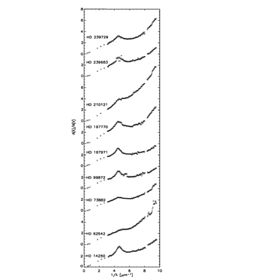
Figure 2: Extinction curves based on the spectral pairs in Figure 1.

We combine data from 2MASS near-infrared photometry (Skrutskie et al., 1997), optical photometry (references are given in Table 1), archival low-dispersion $IUE$ UV spectra processed with the Massa & Fitzpatrick (2000) method, and $FUSE$ FUV spectra for our target sight lines; the spectra were binned to 5 Å. We determined extinction curves from those data using the pair method (Massa, Savage & Fitzpatrick, 1983). The spectral matches between the reddened and comparison stars have been rigorously evaluated by examining their spectra in the IR through UV spectral regions. The stellar pairs used for this study are shown in Figure 1 where the spectrum of the reddened star in each pair lies below the comparison star’s spectrum. The FUSE data, at wavenumbers greater than 8.4 $\mu$m^-1, obviously have lower signal-to-noise as compared to the longer wavelength data. Our method for assembling the complete extinction curves from the IR to the FUV follows that of Gordon et al. (2003) and Gordon & Clayton (1998). The derived extinction curves for each pair are shown in Figure 2. Note that the curves have a smooth transition from the IUE to FUSE wavelengths around 8.4 $\mu$m^-1.

2.4 The Maximum Entropy Method Algorithm

We employ the Maximum Entropy Method (MEM) algorithm for fitting the extinction curves as developed by Kim, Martin & Hendry (1994; hereafter KMH), with slight modifications to facilitate application to the FUSE data. Additional information regarding the MEM implementation may also be found in Hendry & Mochnacki (2000). As recommended by KMH, we use the “mass distribution” – m(a) da = mass of dust grains in the grain-radius interval a to a+da – instead of the more traditional number of grains or “size distribution.” In this form, the classical MRN-type model (Mathis, Rumpl & Nordsieck, 1977) becomes $m(a)\propto a^{-0.5}$. The grain sizes are divided into 50 logarithmically-spaced bins over the range 0.0025-2.7 µm. As discussed by KMH, the shape of the mass distribution is strongly constrained only for data over the region $\sim$0.02-1 µm. Below a size of 0.02 µm, the extinction even in the ultraviolet becomes increasingly dominated by absorption as sizes approach the small-particle (Rayleigh) limit and thus constrains only total mass. Above 1 µm, the “gray” nature of opacity (i.e., extinction efficiency approaching 2) provides a similar type of integral constraint (on surface area). Thus there is danger of a large unconstrained mass if the default mass distribution used in the definition of entropy is not well chosen. We therefore specify the defaults (templates) using the functional form of a power-law with an exponential decay above some characteristic large size $a_{b}$ (PED, see KMH): $m(a)\propto\ a^{-p}exp(-a/a_{b})$. The PED is essentially the traditional gamma distribution function.

The “observations” to which the model is fit are taken from the FM parameterization of the UV data and from the visible/infrared extinction data, resampled at 34 wavelengths. For model wavelengths longward of the observed data, the extinction is calculated using the CCM relation. However, their inclusion in the modeling effort is an artifact of the current MEM implementation, and we do not wish for them to contribute to the resulting mass distributions. As a result, their errors are set to a large number that effectively reduces their weight to zero. The “errors” that are used to weight the data in the MEM algorithm are calculated to represent only the scatter or random errors in the extinction curve. In the visible and infrared, these values are taken directly from the random error estimate produced during the extinction curve generation. Unfortunately, the same approach for the UV points tends to produce “errors” which are much smaller than the point-to-point scatter in the data. As a result, for each model UV bin we have adopted the average deviation of the FM curve from the actual extinction data.

In this work, we consider (only) three-component models of homogeneous, spherical grains: modified “astronomical silicate” Weingartner & Draine (2001), amorphous carbon (Zubko et al., 1996), and graphite (Laor & Draine, 1993), with mass densities ($\rho$) of 3.3 g/cm³, 1.8 g/cm³, and 2.3 g/cm³, respectively. The graphite component is included, as in many models of interstellar extinction, to produce the extinction bump at 2175 Å. Only small graphite particles are appropriate for this purpose, and so for that component we chose $a_{b}=0.02$ µm, much smaller than for the other components ($a_{b}=0.25$ µm). At each wavelength, the appropriately-weighted grain cross section is integrated for each bin (and for each separate composition, see equation 1 in KMH). In order to incorporate abundance constraints (see below), these are expressed as extinction per unit H column density (accounting for H i and H₂).

The total mass of dust is limited by the observed dust-to-gas ratio and “cosmic” abundances. The MEM algorithm includes explicit constraints that do not allow the model to use more carbon or silicon than is “available”. The cosmic abundances adopted were 358 C and 35 Si atoms per million H. The C abundance is an estimate from young F and G stars (Sofia & Meyer, 2001), and the Si abundance is solar (Holweger, 2001). We note that the cosmic C abundance used here is generous; recent results suggest that the solar C/H may be as low as $245\pm 23$ C per million H (Allende Prieto et al., 2002). In order to allow generally for observed carbon gas-phase abundances, we require that no more than 70% of the adopted cosmic C may be used (i.e., 251 C per million H), whereas we allow up to 120% of the cosmic Si (i.e., 42 Si per million H). These relaxed constraints allow for uncertainties in abundances and depletion, and in the dust-to-gas ratio (here $A_{V}/N[H_{tot}]$). Note that the model does not have to use this much C or Si, but often does.

To provide consistency between the individual analyses, we use the same abundance constraints, defaults, and initial guesses of the mass distribtion (to which the model is not particularly sensitive). In order to isolate the effect of including the FUSE data in the analyses, each model is run with and without the FUSE data, (the latter case giving no weight to data beyond 8.7 µm^-1). The MEM algorithm proceeds iteratively to find mass distributions which reproduce the data. The goodness of fit is judged by a reduced-$\chi^{2}$, the “target” value of which should be close to unity for an acceptable solution (we used 1.0 as our target). In the MEM algorithm used, this value is a constraint (along with abundance limits, which must be satisfied for any solution to be considered valid. In other words, a successful MEM solution will have a reduced-$\chi^{2}$ equal to the target value. The assessment of goodness of fit is relative to the adopted errors, and so it is important that these be appropriately calculated (systematic errors are not included). From this point of view, our assessment of random error (see above) appears reasonable, producing “good” fits for a reduced-$\chi^{2}=1$.

3 Discussion

3.1 Sight line characteristics

The basic characteristics of the nine sight lines used in this study are shown in Table 2. The reddened sight lines cover a wide range of Galactic environments as indicated by the large spread in $R_{V}$ values, from 2.43 to 3.81 (see Table 2). These values of $R_{V}$ were determined using a $\chi^{2}$ minimization method; see Gordon et al. (2003) for the details of the method and associated uncertainties. As noted in the introduction, the extinction along these sight lines is unusual compared to a typical line of sight measured in the local interstellar medium. Nevertheless, the sight lines toward HD 14250, HD 73882, HD 99872, HD 167971, HD 239729, and HD 239683, though having different values of $R_{V}$, are still fit well by CCM (Valencic et al., 2004). HD 14250 and HD 73882 were part of the original CCM sample.

HD 239729 and 239683 are in Trumpler 37 along with HD 204827 but do not share any of the anomalous properties of the dust in the latter sight line (Valencic et al., 2003).

HD 197770 shows a broad, weak spectral feature in the ultraviolet interstellar linear polarization centered close to 2175 Å bump (Martin et al., 1995; Wolff et al., 1997; Clayton et al., 1992). HD 197770 is an evolved, spectroscopic, eclipsing binary with two B2 stars (Gordon et al., 1998). The star seems to lie on the edge of a large area of molecular clouds and star formation including Lynds 1036 and 1049 in the Cygnus region (Gordon et al., 1998). On the IRAS maps there is a bright 60 µm shell, 14′ in radius centered on HD 197770, surrounded by an apparent bubble cleared of dust with a radius of approximately 24′ (Gaustad & van Buren, 1993; Gordon et al., 1998).

Only five Galactic sight lines (HD 29647, HD 62542, HD 204827, HD 210121, and HD 283809) are known to show systematic deviations from CCM, excluding the FUV (Valencic et al., 2003, 2004; Clayton et al., 2003b); these sight lines all sample dense, molecule-rich clouds. Two of these sight lines, toward HD 62542 and HD 210121, both of which show strong UV extinction, are included in our data set. The gas toward HD 62542 is rich in CN and CH molecules (Cardelli et al., 1990), and the sight line lies on the edge of material swept up by a stellar wind bubble. The dust in the molecular cloud associated with HD 210121 (Larson, Whittet & Hough, 1996; Larson et al., 2000) seems likely to have been processed too as it was propelled into the halo during a Galactic fountain or other event. As for HD 62542, the non-CCM extinction curve toward HD 210121 has a weak bump, and an even steeper FUV rise, indicating size distributions that are skewed toward small grains (Valencic et al., 2003, 2004), possibly from exposure to shocks or strong UV radiation that disrupted large grains.

3.2 FM and CCM Extrapolation to the FUV

The empirical six-parameter FM relationship well reproduces Galactic UV extinction curves up to 8.7 $\mu$m^-1. CCM is able to reliably predict extinction curves up to 8.7 $\mu$m^-1 with the exception of $\sim 1\%$ of observed Galactic sight lines (Valencic et al., 2004). An extension of these relationships into the FUV would be valuable for correcting extinction effects. In addition, a valid extension of CCM would be especially important because of its ability to predict (to some degree) the extinction curves based on ground-based photometric parameters alone. Figures 3a and 3b show the extinction curves for our sample superimposed with three fits to each. The fits include each: an FM fit based on IUE data alone, an FM fit based on IUE and FUSE data, and a CCM fit based on the measured value of $R_{V}$ = A_V/E(B-V).

Each of the Galactic extinction curves in our sample is well reproduced by FM curves fitted to data in the IUE and FUSE wavelength regions. The six parameters used for these FM fits are shown in Table 3. The good agreement between the extinction curves and FM fits in the FUV is not necessarily expected given that Fitzpatrick & Massa (1990) based their empirical fit to the extinction curves on data that went up to only 8.7 $\mu$m^-1 (i.e., only in the IUE wavelength region). Fitzpatrick & Massa (1988) found that the curvature of the extinction curve from 5.9 - 8.7 $\mu$m^-1 always has the same shape regardless of the dust size distribution or physical environment. Our small sample of sight lines suggest that this relationship extends to the FUV and that the extinction curve from 5.9 - 9.5 $\mu$m^-1 can be fit with a single continuous function; the same function found by Fitzpatrick & Massa (1988). The continuity of the curvature shape at wavenumbers above 8.7 $\mu$m^-1 is verified by the fact that the FM fits based on the IUE data alone are, in most cases, indistinguishable from the FM fits to the combined IUE and FUSE data (the solid and dotted lines in Figure 3). The largest deviation between the two FM fits for a given extinction curve occurs for HD 197770 where the fits differ by less than 0.5 magnitudes at 9.5 $\mu$m^-1; this is within the expected uncertainty for this noisier portion of the extinction curve. Analysis of our sample suggests that FM fits can be extrapolated safely from IUE wavelengths up to 9.5 $\mu$m^-1. Fitzpatrick & Massa (1988) propose that the stability of the extinction curve shape at short wavelengths results only from a dust component optical property, as opposed to a function involving grain size. While we certainly find a similar behavior in shape of the extinction curve from 1050 - 1700 Å, we cannot exclude the possibility of systematic variations in particle sizes as viable mechanisms.

For these lines of sight, selected for their unusual extinction, the predictive capability of the CCM relationship for FUV extinction is more problematic. Note, however, that in contrast to the FM fits, no ultraviolet data, neither UV nor FUV, are used to determine the single CCM fitting paramater $R_{V}$; thus the ability to predict the UV extinction for most stars is a remarkable feature of CCM. For the two sight lines in our sample where CCM does not match even the UV extinction, toward HD 62542 and HD 210121, it also fails to reproduce the FUV. This is not a surprising result since the longer wavelength data already suggested that the grains in these sight lines have likely experienced processing that is different from that in more “average” Galactic sight lines. The departure from the CCM relationship grows with increased wavenumber over the measured region up to a maximum of about 3 magnitudes per A_V at 9.5 $\mu$m^-1; for HD 62542 and HD 210121, CCM underpredicts the FUV extinction as much as 40% and 35%, respectively. HD 62542 is known to have an anomalous 2175Å bump – unusually weak and peaking at an atypically high wavenumber; Cardelli & Savage (1988) find $x_{0}=4.74\micron^{-1}$ and we find $x_{0}=4.78\pm 0.08\micron^{-1}$. This suggests that the failure of CCM to reproduce the FUV extinction may be associated with anomalous properties of the particles producing the 2175 Å bump along this sight line.

The sight lines toward four stars, HD 73882, HD 99872, HD 167971 and HD 239729, are, within uncertainties, well represented by CCM over the IR to UV wavelength region, but much less so in the FUV. The CCM functions for these sight lines differ from the well-fit FM curves by 2 $\sigma$ or more (based on the $R_{V}$ uncertainties) at 9.5 $\mu$m^-1. As with the HD 62542 and HD 210121 extinction curves, the differences between the CCM predictions and the measurements increase with increasing wavenumber. The fact that CCM fits the extinction curves in the IR through UV, but diverges in the FUV may indicate that the systematic processing of larger grains does not necessarily continue to the small grain population, at least in the same way. CCM FUV extinction in two of these sight lines (HD 73882 and HD 239729) is too high while it is too low in the other two (HD 99872 and HD 167971). The $R_{V}$ values for this group of four sight lines ranges from 2.99 to 3.81.

The final three sight lines in our sample, toward HD 14250, HD 197770 and HD 239683, have CCM curves that predict well the FUV extinction. The $R_{V}$ values of these three sight lines range from 2.44 to 2.98; smaller than the group for which CCM did poorly. While one might suggest that CCM can be extrapolated into the FUV more reliably for smaller $R_{V}$ values and the potential connection to an increased relative abundance of small grains, further generalization awaits a larger sample of FUV extinction (as will be presented in Paper III).

3.3 MEM Grain Models

The resulting model-data comparisons are presented in Figure 4, which shows the amount of extinction provided by each of the three materials and the total extinction of the model compared to the measured extinction curve. The percentages of the carbon and silicon along the sight lines that are used to produce the displayed fits are given in Table 4.

Our models use three grain types to reproduce the observed extinction, specifically astronomical silicates, amorphous carbon, and graphite. A more realistic dust model would include other compositions such as oxides and grains composed of a combination of carbonaceous and silicaceous materials. It would also account for non-spherical particles and the effects of coatings on and vacuums in the grains. We have chosen to use a simple model here because of the computational complexity and arbitrary assumptions often associated with a more physically complete approach (Clayton et al., 2003a). By doing so, we acknowledge that the detailed results of the models, such as specific populations of grain types and sizes, and the abundance constraints that they imply, are to be used with caution. However, these simple models can provide some useful information about dust. Since the absorption characteristics of a grain may be well constrained by its bulk behavior, the models can provide estimates of the mass distribution among grain-size populations that are appropriate to more complex systems.

The left and right columns in Figure 4 show the MEM fits to the extinction curves based on data up to 9.5 $\mu$m^-1 (FUSE wavelengths), and 8.7 $\mu$m^-1 (IUE wavelengths), respectively. Although some of the FUV extinction is produced by the grains that are also responsible for extinction at longer wavelengths, it is clear that models based on data only to 8.7 $\mu$m^-1 do not always fit the FUV extinction well. Other than toward HD 167971 and HD 197770, the extinction curves require a larger fraction of grain material to be in small dust particles, mostly silicates in our model, to adequately account for the FUV. More specifically, within the context of our simple three-component model, the inclusion of the FUV requires up to 10% more silicon to be in grains (see Table 4). Since the FM parameter $c_{4}$ is a measure of the strength of the far UV rise in an extinction curve, it is not surprising that we find a correlation between this value and an increased need for small silicate grains. A linear fit to this relationship (a higher-order polynomial is not statistically justifiable) indicates that in order to fit the FUV constraint, 12% more silicon is needed per increase of 1.0 in $c_{4}$; the $1\sigma$ scatter about the line is a 2% change in the required silicon. The largest portion of the scatter is likely attributable to the errors assigned to the extinction curve data (see §2.4). Since the models tend to underfit the extinction when less constrained (when the data have larger uncertainties; see the left panels in Figure 4), we are likely underestimating the extra mass needed in small silicates for our simple model to fit the FUV. The fraction of C allocated to amorphous carbon grains often decreases in the models that include the FUV extinction constraint (see Table 4); amorphous carbon serves as a source of visible opacity in these models. On the other hand, the abundance of C that the models allocate to graphite grains is often enhanced when the FUV is included. This general increase in graphite and decrease in amorphous carbon represents the model’s reallocation of C to fit better the extinction out to 9.5 µm^-1; the upward curvature in the graphite extinction at wavenumbers greater than 8 $\mu$m^-1 fits the upward turn often seen in the extinction curves at these wavelengths. Nevertheless, one should also consider the possibility that there is something wrong with the dielectric function of our silicate component in not being able to produce this upward curvature, or perhaps that other components missing entirely, e.g., PAHs, nanoparticles.

We note that the fits to x $<9.5$ µm^-1 in Figure 4 are often poorest in the FUV where the models tend to underestimate the extinction. Since a disproportionate share of the target $\chi^{2}$ is coming from the FUV, we have experimented with lowering the target reduced-$\chi^{2}$ in the models to better fit this region. We show two examples of forcing a tighter FUV fit in Figure 5. The figure displays three MEM models for the sight lines toward HD 62542 and HD 210121, one based on each: data up to 8.7 µm^-1 with a reduced-$\chi^{2}=1.0$, data up to 9.5 µm^-1 with a reduced-$\chi^{2}=1.0$, and data up to 9.5 µm^-1 with a reduced-$\chi^{2}=0.5$. The left panels show the fits to the data for each model. The right panels show the resultant mass distribution of each component relative to the mass of hydrogen. The reduced-$\chi^{2}=1$, x $<9.5$ µm^-1 model for HD 62542 does not use all of the Si or C available to it, so the model can draw on both of these elements when it tries to fit better the FUV data (see Table 4). The reduced-$\chi^{2}=0.5$ model does, in fact, take the entire allocation of Si (120%), however it uses less of the available C than the less-constrained fit; specifically, the more-constrained model puts 30% of the total carbon abundance into amorphous C and 7% into graphite. The top right panel of Figure 5 shows that much of the “extra” silicon used to fit better the FUV was put into small grains. The grain sizes below 200 Å are not well resolved, so the shape of the mass curve at these small sizes is guided by the model template and not the actual distribution in size. However, the changes in the overall mass of grains below 0.02 $\mu$m, as shown in the figure, are significant. Figure 5 also shows that the model is reallocating the size distributions of the grains so that, for instance, the graphite is contributing more extinction at 2175 Å relative to the amorphous carbon (note the decrease in amorphous carbon grains with sizes around 0.2 µm as the FUV is better fit). Recall however that at reduced-$\chi^{2}=0.5$, the model is overconstrained if our treatment of the errors is appropriate. We caution against overinterpreting these size distribution results; we present them merely to show that this simplified model requires changes in the grain size distributions in order to better fit the FUV.

The reduced-$\chi^{2}=1$ model for HD 210121 uses the maximum available Si, so it can only draw on C in order to put more mass into grains for a better FUV fit. The reduced-$\chi^{2}=0.5$ model continues to incorporate the maximum allocated Si, and increases the C that it uses for each of the amorphous carbon grains and graphite by 1% of the total C abundance. This overconstrained model is able to fit the extinction primarily by reallocating the size-distributions of the grains in a way that is similar to the reduced-$\chi^{2}=0.5$ model for HD 62542. A rigorous analysis that relates grain size distributions to extinction will require a more complex model as well as extinction curves with smaller uncertainties in the FUV.

4 Summary

1. We present the extinction curves from the IR to the FUV (up to 9.5 $\mu$m^-1) for nine Galactic sight lines observed with FUSE.

2. The FUV extinction curves out to 9.5 $\mu$m^-1 are all well fit with an extrapolation of the FM relationship (Fitzpatrick & Massa, 1990) from the IUE wavelength range that extends to only 8.7 $\mu$m^-1.

3. The CCM relationship (Cardelli, Clayton, & Mathis, 1989) does not properly predict the FUV extinction in the two sight lines in our sample where it also fails to reproduce the IR – UV extinction.

4. CCM does fit the IR – UV in seven of our sight lines. For three of these, all with $R_{V}$ values below the Galactic average, an extrapolation of CCM does properly predict the FUV extinction. The other four sight lines all have larger $R_{V}$ values than the previous group. An extrapolation of CCM over-predicts the FUV extinction in two of these sight lines, and under-predicts it in the other two.

5. Our simple MEM grain models are generally able to fit the extinction curves that include the FUV constraints. The more highly constrained models usually require more mass to be in small grains (radii $\lesssim 200$ Å) in order to reproduce an extinction curve that includes the IR – FUV as compared to those using only the IR – UV.

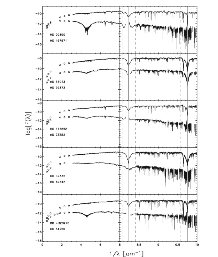
Figure 1: The infrared to far ultraviolet spectra of our sample pairs. The comparison and reddened stars are the upper and lower spectra in each panel, respectively. The solid vertical lines show the locations of H i absorption and the dashed vertical lines show the width of those features. The effects of H₂ absorption have been removed from the spectrum where the absorption is less than or equal to 30% of the continuum level. The spectra are not plotted where the H₂ features absorb more than 30% of the continuum.

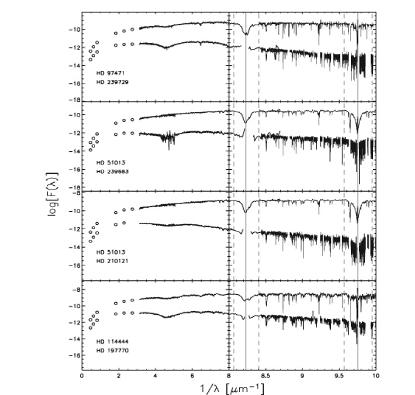
Figure 1b: The same as Figure 1a.

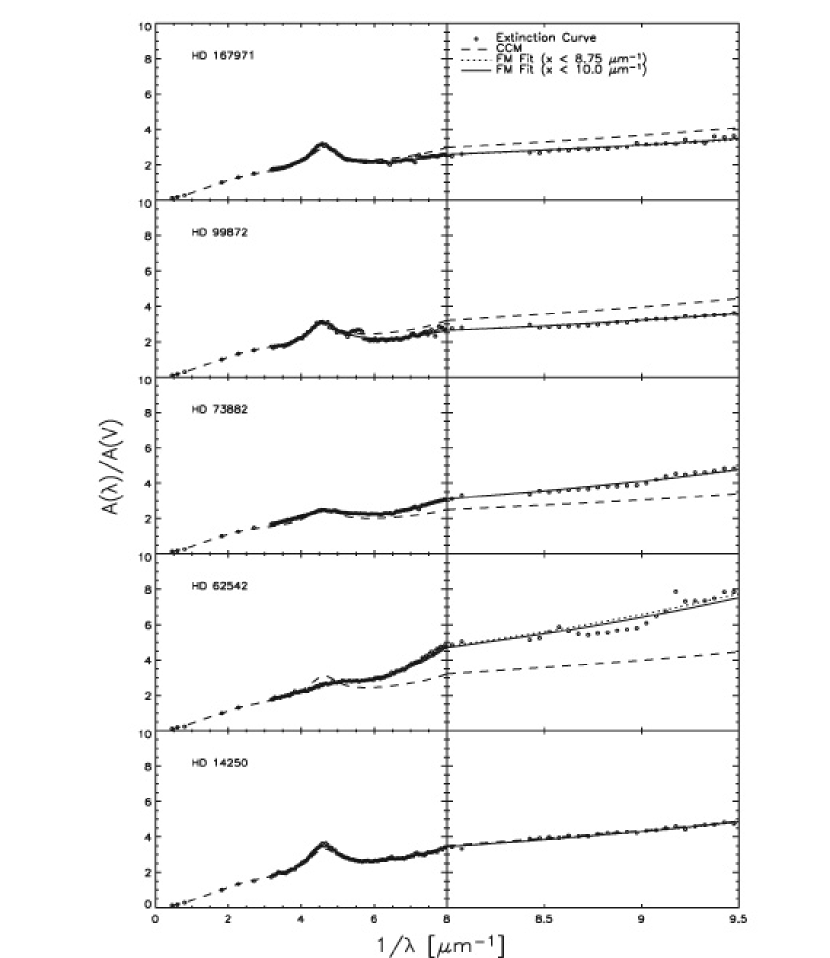
Figure 3: The figure shows CCM and FM fits to the extinction curves; the circles represent the measured extinction. The solid line that represents the FM curves based on fits out to 9.5µm^-1 are difficult to see because they so closely follow the extinction curves. The dotted line that represents the FM fit based only on data below 8.7 µm^-1 is usually indistinguishable from the FM fit out to 9.5 µm^-1. The dashed lines represent CCM curves based on the measured $R_{V}$ values along the sight lines (see Table2).

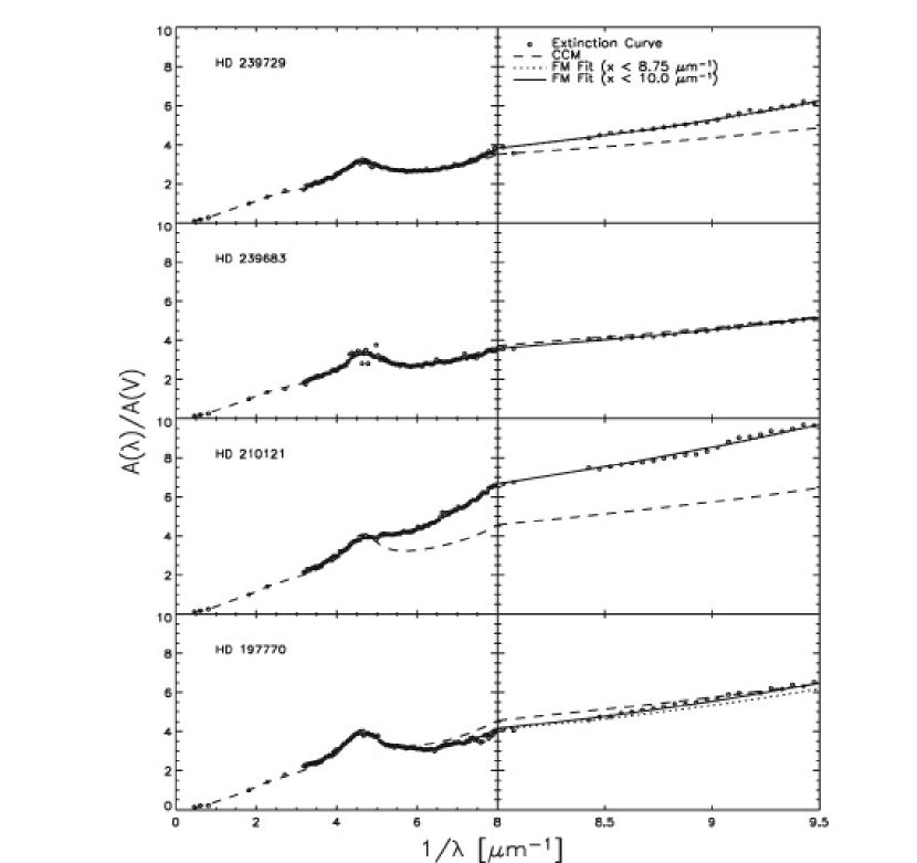
Figure 3b: The same as Figure 3a.

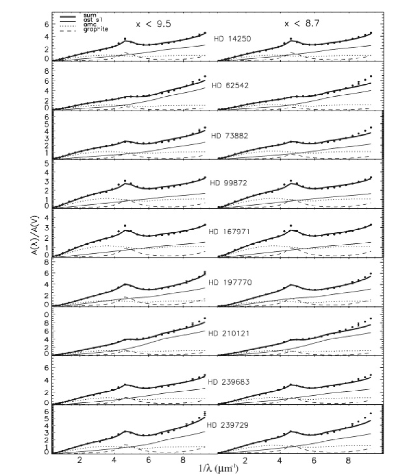
Figure 4: The extinction curve fits resulting from the MEM modeling. The models that fit out to the FUV (x $<9.5$ µm^-1) are shown in the left panel, and those fit out to only the UV (x $<8.7$ µm^-1) are on the right. The 1-$\sigma$ error bars (see §4.1) are shown on every third point when they are larger than the point itself. The circles are the FM fits to the data out to 9.5 µm^-1 (see Table 3). The thick solid line is the total extinction from three components: astronomical silicate (narrow solid line), amorphous carbon (dotted line) and graphite (dashed line) grains. The fractions of silicon and carbon that the model incorporates into the different grain types are listed in Table 4.

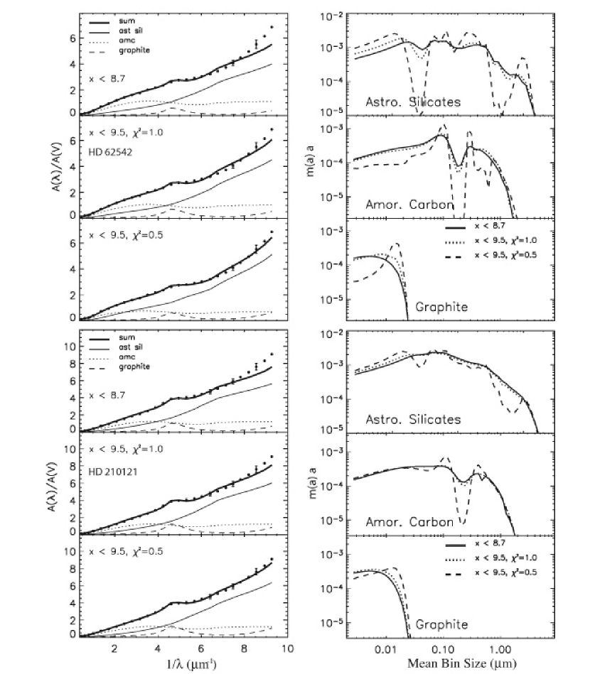
Figure 5: MEM extinction fits (left panels) and mass distributions as a function of grain size (right panels) for the sight lines toward HD 62542 (upper panels) and HD 210121 (lower panels). MEM models are shown for fits out to the UV data only (x $<8.7$ µm^-1) with a reduced-$\chi^{2}=1.0$, for fits out to the FUV (x $<9.5$ µm^-1) with a reduced-$\chi^{2}=1.0$, and for fits out to the FUV with a reduced-$\chi^{2}=0.5$. The panels on the right show the distribution of grain sizes found for the three dust types modeled.

Table 1: Obervations

Sight line	FUSE	Exposure	Mode	Optical data
	targets	(sec)		references
BD+32 270	A063-07	4,900	HIST	1
HD 14250	A118-06	8,200	TTAG	2
HD 37332	B060-12	2,300	HIST	3
HD 51013	A063-09	4,100	HIST	4
HD 62542	P116-02	11,400	TTAG	5
HD 73882	X021-03	25,500	TTAG	6
	P116-13	13,600	TTAG
HD 97471	A118-04	4,200	HIST	7
HD 99872	A120-06	3,300	HIST	5
HD 99890	P102-46	4,600	HIST	7
HD 114444	A118-05	5,500	TTAG	8
HD 116852	P101-38	5,100	HIST	8
HD 167971	P116-21	9,500	TTAG	9
HD 197770	A118-13	6,000	TTAG	10
HD 210121	P116-30	13,800	TTAG	11
HD 239683	A118-10	9,200	TTAG	12
HD 239729	A118-07	9,900	TTAG	12

Table 2: Observational Characteristics of Sight Lines.

		Reddened			Comparison
Reddened	Comparison	Sp T	$N_{H_{2}}$a		Sp T	$N_{H_{2}}$	RV	$\Delta$(B-V)	$\Delta N_{HI}$	H i Referencesb
sight line	sight line		($10^{20}cm^{-2}$)			($10^{20}cm^{-2}$)		(mag)	($10^{21}cm^{-2}$)
HD 14250	BD+32 270	B1 IV	5.5		B2 V	$\cdots$	2.98$\pm$0.14	0.48$\pm 0.05$	1.57$\pm$0.28	1
HD 62542	HD 37332	B5 V	6.5		B5 V	$\cdots$	3.18$\pm$0.22	0.31$\pm$0.03	1.53$\pm$0.17	2
HD 73882	HD 116852	O9 III	12.9		O9 III	0.62	3.81$\pm$0.16	0.49$\pm$0.02	1.29$\pm$0.53	3
HD 99872	HD 51013	B3 V	3.5		B3 V	$\cdots$	3.20$\pm$0.22	0.31$\pm$0.03	0.60$\pm$0.15	1
HD 167971	HD 99890	B0 V	7.1		B0.5 V	$\cdots$	3.37$\pm$0.09	0.81$\pm$0.03	3.99$\pm$0.27	2,4
HD 197770	HD 114444	B2 III	10.7		B2 III	$\cdots$	2.44$\pm$0.15	0.37$\pm$0.02	0.63$\pm$0.05	1
HD 210121	HD 51013	B3 V	5.6		B3 V	$\cdots$	2.43$\pm$0.16	0.35$\pm$0.05	1.41$\pm$0.32	1
HD 239683	HD 51013	B3 IV	5.6		B3 V	$\cdots$	2.86$\pm$0.15	0.43$\pm$0.03	2.00$\pm$0.47	1
HD 239729	HD 97471	B0 V	11.8		B0 V	0.80	2.99$\pm$0.18	0.37$\pm$0.04	1.82$\pm$0.22	2

Table 3: Parameters for Fitzpatrick & Massa Fits to the Extinction Curves

Sight line	c1	c2	c3	c4	x0	$\gamma$
HD 14250
x $<$ 9.5 µm-1	-0.351	0.779	3.945	0.454	4.593	0.941
error	1.031	0.082	0.507	0.044	0.010	0.022
x $<$ 8.7 µm-1	-0.352	0.780	3.942	0.448	4.593	0.941
error	0.079	0.076	0.451	0.052	0.012	0.016
HD 62542
x $<$ 9.5 µm-1	-1.240	1.253	0.446	1.047	4.780	0.798
error	0.395	0.141	0.124	0.128	0.080	0.014
x $<$ 8.7 µm-1	-1.203	1.242	0.486	1.131	4.787	0.826
error	0.401	0.146	0.137	0.158	0.080	0.014
HD 73882
x $<$ 9.5 µm-1	0.879	0.593	3.123	0.810	4.603	1.248
error	0.219	0.046	0.266	0.046	0.030	0.021
x $<$ 8.7 µm-1	0.817	0.604	3.168	0.800	4.600	1.254
error	0.163	0.040	0.234	0.049	0.020	0.020
HD 99872
x $<$ 9.5 µm-1	0.101	0.488	5.830	0.360	4.590	1.180
error	0.038	0.080	1.310	0.097	0.076	0.020
x $<$ 8.7 µm-1	0.097	0.487	5.862	0.370	4.590	1.182
error	0.033	0.081	1.312	0.115	0.076	0.020
HD 167971
x $<$ 9.5 µm-1	1.538	0.330	2.811	0.381	4.577	0.808
error	0.256	0.050	0.288	0.038	0.021	0.013
x $<$ 8.7 µm-1	1.450	0.347	2.826	0.351	4.575	0.810
error	0.249	0.044	0.277	0.044	0.018	0.013
HD 197770
x $<$ 9.5 µm-1	1.217	0.517	5.359	0.733	4.616	1.233
error	0.326	0.056	0.586	0.058	0.032	0.021
x $<$ 8.7 µm-1	1.112	0.546	5.115	0.637	4.609	1.207
error	0.298	0.053	0.496	0.083	0.030	0.020
HD 210121
x $<$ 9.5 µm-1	-3.296	1.882	1.913	0.672	4.611	1.093
error	0.676	0.262	0.450	0.106	0.066	0.018
x $<$ 8.7 µm-1	-3.314	1.887	1.902	0.663	4.609	1.090
error	0.760	0.268	0.454	0.119	0.064	0.018
HD 239683
x $<$ 9.5 µm-1	0.116	0.703	4.726	0.515	4.614	1.235
error	0.031	0.057	0.601	0.047	0.044	0.022
x $<$ 8.7 µm-1	0.137	0.699	4.738	0.523	4.616	1.237
error	0.077	0.050	0.560	0.068	0.046	0.025
HD 239729
x $<$ 9.5 µm-1	0.484	0.642	4.342	0.937	4.597	1.219
error	0.102	0.066	0.487	0.098	0.019	0.020
x $<$ 8.7 µm-1	0.462	0.648	4.293	0.916	4.595	1.213
error	0.106	0.067	0.484	0.103	0.016	0.020

Table 4: Percentage of Available Carbon and Silicon used in Models

Sight line	Silicon		Carbon
	AS		AMC	Graphite
HD 14250
x $<$ 9.5 µm-1	114%		51%	24%
x $<$ 8.7 µm-1	112%		51%	24%
HD 62542
x $<$ 9.5 µm-1	99%		36%	8%
x $<$ 8.7 µm-1	90%		37%	7%
HD 73882
x $<$ 9.5 µm-1	90%		53%	14%
x $<$ 8.7 µm-1	84%		55%	12%
HD 99872
x $<$ 9.5 µm-1	121%		76%	24%
x $<$ 8.7 µm-1	120%		77%	24%
HD 167971
x $<$ 9.5 µm-1	73%		54%	16%
x $<$ 8.7 µm-1	73%		54%	16%
HD 197770
x $<$ 9.5 µm-1	85%		32%	18%
x $<$ 8.7 µm-1	85%		35%	16%
HD 210121
x $<$ 9.5 µm-1	120%		36%	14%
x $<$ 8.7 µm-1	119%		36%	12%
HD 239683
x $<$ 9.5 µm-1	78%		41%	16%
x $<$ 8.7 µm-1	77%		42%	15%
HD 239729
x $<$ 9.5 µm-1	60%		27%	12%
x $<$ 8.7 µm-1	57%		28%	10%

References

- Allende Prieto et al. (2002) Allende Prieto, C., Lambert, D. L., & Asplund, M. 2002, ApJ, 573, L137
- Bohlin (1975) Bohlin, R. C. 1975, ApJ, 200, 402
- Buss et al. (1994) Buss, R. H, Allen, M., McCandliss, S., Kruk, J., Liu, J., & Brown, T. 1994, ApJ, 430, 630
- Cardelli, Clayton & Mathis (1988) Cardelli, J. A., Clayton, G., C., & Mathis, J. S. 1988, ApJ, 329, L33
- Cardelli, Clayton, & Mathis (1989) —–. 1989, ApJ, 345, 245
- Cardelli & Savage (1988) Cardelli, J. A., & Savage, B. D. 1988, ApJ, 325, 864
- Cardelli et al. (1990) Cardelli, J. A., Suntzeff, N. B., Edgar, R. J., & Savage, B. D. 1990, ApJ, 362, 551
- Cartledge et al. (2005) Cartledge, S. I. B., Clayton, G. C., Gordon, K. D., Rachford, B. L., Draine, B. T., Martin, P. G., Mathis, J. S., Misselt, K. A., Sofia, U. J., Whittet, D. C. B., & Wolff, M. J. 2005, ApJ, submitted
- Clayton et al. (1992) Clayton, G. C., Anderson, C. M., Magalhaes, A. M., Code, A. D., Nordsieck, K. H., Meade, M. R., Wolff, M., Babler, B., Bjorkman, K., Schulte-Ladbeck, R. E., Taylor, M., & Whitney, B. A. 1992, ApJ, 385, L53
- Clayton et al. (2003b) Clayton, G. C., Gordon, K. D., Salama, F., Allamandola, L. J., Martin, P. G., Snow, T. P., Whittet, D. C. B., Witt, A. N., & Wolff, M. J. 2003, ApJ, 592, 947
- Clayton et al. (2003a) Clayton, G. C., Wolff, M. J., Sofia, U. J., Gordon, K. D., & Misselt, K. A., 2003 ApJ, 588, 871
- Cousins & Stoy (1962) Cousins, A. W. J., & Stoy, R. H. 1962, R. Obs. Bull., 64, 103
- Denoyelle (1977) Denoyelle, J. 1977, A&AS, 27, 343
- Dworetsky, Whitelock & Carnochan (1982) Dworetsky, M. M., Whitelock, P. A., & Carnochan, D. J., MNRAS, 201, 901
- Feinstein (1967) Feinstein, A. 1967, ApJ, 149, 107
- Feinstein (1969) —–. 1969, MNRAS, 143, 273
- Fitzpatrick (1999) Fitzpatrick, E. L. 1999, PASP, 111, 63
- Fitzpatrick & Massa (1986) Fitzpatrick, E. L., & Massa, D. 1986, ApJ, 307, 286
- Fitzpatrick & Massa (1988) —–. 1988, ApJ, 328, 734
- Fitzpatrick & Massa (1990) —–. 1990, ApJS, 72, 163
- Forbes (1984) Forbes, D. 1984, IAU Inform. Bull. Var. Stars, 2605, 1
- Garrison & Kormendy (1976) Garrison, R. F., & Kormendy, J. 1976, PASP, 88, 865
- Gaustad & van Buren (1993) Gaustad, J. E., & van Buren, D. 1993, PASP, 105, 1127
- Gordon & Clayton (1998) Gordon, K. D., & Clayton, G. C. 1998, ApJ, 500, 816
- Gordon et al. (2003) Gordon, K. D., Clayton, G. C., Misselt, K. A., Landolt, A. U., & Wolff, M. J. 2003, ApJ, 594, 279
- Gordon et al. (1998) Gordon, K. D., Clayton, G. C., Smith, T. L., Aufdenberg, J. P., Drilling, J. S., Hanson, M. M., Anderson, C. M., & Mulliss, C. L. 1998, AJ, 115, 2561
- Green et al. (1992) Green, J. C., Snow, T. P., Cook, T. A., Cash, W. C., & Poplawski, O. 1992, ApJ, 395, 289
- Hardie, Heiser & Tolbert (1964) Hardie, R. H., Heiser, A. M., & Tolbert, C. R. 1964, ApJ, 140, 1472
- Hendry & Mochnacki (2000) Hendry, P. D., & Mochnacki, S. W. 200, ApJ, 531, 467
- Hill, Kilkenny & van Breda (1974) Hill, P. W., Kilkenny, D., & van Breda, I. G. 1974, MNRAS, 168, 451
- Hill & Lynas-Gray (1977) Hill, P. W., & Lynas-Gray, A. E. 1977, MNRAS, 180, 691
- Holweger (2001) Holweger, H. 2001, in Solar and Galactic Composition, ed. R. F. Wimmer-Schweingruber (Berlin:Springer-Verlag), 23
- Hutchings & Giasson (2001) Hutchings, J. B., & Gaiasson, J. 2001, PASP, 113, 1205
- Jenkins, Savage, & Spitzer (1986) Jenkins, E. B., Savage, B. D., & Spitzer, L. 1986, ApJ, 301, 355
- Kim, Martin, & Hendry (1994) Kim, S.-H., Martin, P. G. & Hendry, P. D. 1994, ApJ, 422, 164
- Laor & Draine (1993) Laor, A., & Draine, B. T. 1993, ApJ, 402, 441
- Larson, Whittet & Hough (1996) Larson, K. A., Whittet, D. C. B., & Hough, J. H. 1996, ApJ, 472, 755
- Larson et al. (2000) Larson, K. A., Wolff, M. J., Roberge, W. G., Whittet, D. C. B., & He, L. 2000, ApJ, 532, 1021
- Lewis, Cook & Chakrabarti (2005) Lewis, N. K., Cook, T. A., & Chakrabarti, S. 2005, ApJ, 619, 357
- Longo et al. (1989) Longo, R., Stalio, R., Polidan, R. S., & Rossi, L. 1989, ApJ, 566, 267
- Martin et al. (1995) Martin, P., Sommerville, W., McNally, D., Whittet, D., Allen, R., Walsh, J., & Wolff, M. 1995, in The Diffuse Interstellar Bands, ed. A. G. G. M. Tielens, and T. P. Snow (Dordrecht:Klewer), 271
- Massa & Fitzpatrick (2000) Massa, D., & Fitzpatrick, E. L. 2000, ApJS, 126, 517
- Massa, Savage & Fitzpatrick (1983) Massa, D., Savage, B. D., & Fitzpatrick, E. L. 1983, ApJ, 266, 662
- Mathis, Rumpl & Nordsieck (1977) Mathis, J. S., Rumpl, W., & Nordsieck, K. H. 1977, ApJ, 217, 425
- Mendoza (1967) Mendoza, E. E. 1967, Bol. Obs. Tonantz. Tacub., 4, 149
- Rachford et al. (2002) Rachford, B. L., Snow, T. P., Tumlinson, J., Shull, J. M., Blair, W. P., Ferlet, R., Friedman, S. D., Gry, C., Jenkins, E. B., Morton, D. C., Savage, B. D., Sonnentrucker, P., Vidal-Madjar, A., Welty, D. E., & York, D. G. 2002, ApJ, 577, 221
- Rachford et al. (2001) Rachford, B. L., Snow, T. P., Tumlinson, J., Shull, J. M., Roueff, E., Andre, M., Desert J. M-., Ferlet, R., Vidal-Madjar, A., & York, D. G. 2001, ApJ, 555, 839
- Sahnow (2003) Sahnow, D. J. 2003, in Future EUV/UV and Visible Space Astrophysics Missions and Instrumentation, ed. J. C. Blades, & O. H. W. Siegmund, (Bellingham: International Society for Optical Engineering), 610
- Sahnow et al. (1996) Sahnow, D. J., Friedman, S. D., Oegerle, W. R., Moos, H. W., Green, J. C., & Siegmund, O. H. 1996, in Space Telescopes and Instruments IV, ed. P. Y. Bely, & J. B. Breckinridge, (Bellingham: International Society for Optical Engineering), 2
- Sasseen et al. (2002) Sasseen, T. P., Hurwitz, M., Dixon, W. V., & Airieau, S. 2002, ApJ, 566, 267
- Savage & Mathis (1979) Savage, B. D., & Mathis, J. S. 1979, ARA&A, 17, 73
- Skrutskie et al. (1997) Skrutskie, M. F., et al., in The Impact of Large Scale Near-IR Sky Surveys, (Dordrecht:Klewer), 25
- Snow, Allen & Polidan (1990) Snow, T. P., Allen, M. M., & Polidan, R. S. 1990, ApJ, 359, L23
- Snow & York (1975) Snow, T. P., & York, D. G. 1975, Ap&SS, 34, 19
- Sofia & Meyer (2001) Sofia, U. J., & Meyer, D. M. 2001, ApJ, 554, L221
- Valencic et al. (2003) Valencic, L.A., Clayton, G.C., Gordon, K.D., & Smith, T.L. 2003, ApJ, 598, 369
- Valencic et al. (2004) Valencic, L.A., Clayton, G.C., & Gordon, K.D. 2004, ApJ, 616, 912
- Weingartner & Draine (2001) Weingartner, J.C., & Draine, B.T. 2001, ApJ, 548, 296
- Welty & Fowler (1992) Welty, D. E., & Fowler, J. R. 1992, ApJ, 393, 193
- Wolff et al. (1997) Wolff, M.J., Clayton, G.C., Kim, S.H., Martin, P.G., & Anderson, C.M. 1997, ApJ, 478, 395
- York et al. (1973) York, D. G., Drake, J. F., Jenkins, E. B., Morton, D. C., Rogerson, J. B., & Spitzer, L. 1973, ApJ, 182, L1
- Zubko et al. (1996) Zubko, V. G., Mennella, V., Colangeli, L., & Bussoletti, E.,1996, MNRAS, 282, 1321