The baryonic mass function of galaxies

Abstract

mass function, stellar, HI, gas, baryonic

In the Big Bang about 5% of the mass that was created was in the form of normal baryonic matter (neutrons and protons). Of this about 10% ended up in galaxies in the form of stars or of gas (that can be in molecules, can be atomic, or can be ionised).

In this work, we measure the baryonic mass function of galaxies, which describes how the baryonic mass is distributed within galaxies of different types (e.g. spiral or elliptical) and of different sizes. This can provide useful constraints on our current cosmology, convolved with our understanding of how galaxies form. This work relies on various large astronomical surveys, for example the optical Sloan Digital Sky Survey (to observe stars) and the HIPASS radio survey (to observe atomic gas). We then perform an integral over our mass function to determine the cosmological density in baryons in galaxies: $\Omega_{\rm b,gal}=0.0035$. Most of these baryons are in stars: $\Omega_{*}=0.0028$. Only about 20% are in gas. The error on the quantities, as determined from the range obtained between different methods, is $\sim 10$%; systematic errors may be much larger.

Most ($\sim 90$%) of the baryons in the Universe are not in galaxies. They probably exist in a warm/hot intergalactic medium. Searching for direct observational evidence and deeper theoretical understanding for this will form one of the major challenges for astronomy in the next decade.

1 Introduction

The hot Big Bang theory is the current paradigm for the formation and evolution of the Universe. Parts of the theory that describe the Universe in the first small fraction of a second, like superstring theory, cannot rigorously be tested by experiment and so are not well-constrained at present. But the parts that describe the subsequent evolution of the Universe have been very successful. Examples of the successes are the predictions of the cosmic microwave background (CMB), the abundances of light elements and the expansion of the Universe (Peacock, 1999).

One feature of the model is the partitioning of mass-energy into entities that obey different equations of state. In Table 1, we list current estimates for the densities of these forms of mass-energy (Fukugita & Peebles 2004, Allen et al. 2004). These numbers come from matching the theory to observations of the CMB (e.g. Spergel et al. 2003), the distance-redshift relation obtained from Type Ia supernova (e.g. Riess et al. 2004), and observations of rich galaxy clusters a different redshifts (Allen et al. 2004). The two main components are a dark energy component with density $\Omega_{\Lambda}$, which could be a cosmological constant, and a matter component with density $\Omega_{M}$. The matter density can further be divided into a dark-matter component and a baryonic component. Inferences about the density of the baryonic component come from observations of the CMB angular power spectrum (Spergel et al., 2003) and the abundances of light elements D, ³He, ⁴He and ⁷Li (Coc et al. 2004) when compared with big bang nucleosynthesis theory (BBN). The existence of the dark matter component is strengthened by independent evidence from the dynamics and clustering of galaxies and clusters of galaxies (e.g. de Blok et al. 2001, Kleyna et al. 2001 and Borriello & Salucci 2001); and from gravitational lensing measurements (Mellier 1999 and Sand et al. 2004). The baryonic component is the subject of the present paper.

Table 1: Composition of the Universe

Total density Dark energy density

$$\Omega=1$$

Matter density Dark matter density

Baryonic density

Understanding the present distribution of material in the Universe is a formidable challenge. With the advent of fast computers and efficient algorithms for calculating the force between many particles, we can now make solid predictions for the current distribution of dark matter (Bertschinger 1988). However, understanding the distribution of stars and gas is more difficult. This involves a detailed understanding of the physics underlying galaxy formation: gas hydrodynamics, star formation, and feedback from exploding stars and forming black holes. Despite these difficulties, much progress has been made and simulations are now on the verge of being able to make predictions about where and in what form we should expect to find baryons in the universe today (see e.g. Mayer 2004 and Springel et al. 2005). The new hydrodynamic simulations of galaxy formation (e.g. Davé et al. 2001 and  Nagamine et al. 2005) include an intergalactic medium, which makes it straightforward to include these effects.

Technological advances in observational astronomy have also been rapid, mainly as regards our ability to compile and process large datasets. The results from many surveys have recently been published. These include optical redshift surveys, like the Sloan Digital Sky Survey (SDSS; Abazajian et al. 2004) and the 2DF Galaxy Redshift Survey (Colless et al., 2001), near-infrared photometric surveys like 2MASS (Gao et al. 2004), and HI atomic gas surveys like HIPASS (Koribalski et al. 2004).

The time, therefore, is ripe to use the survey results in conjunction with each other to calculate precisely the distribution of baryons in the Universe. This will then provide a valuable resource against which cosmological simulations which include the complex physics of star formation and galaxy formation may be tested. It also presents a vital census of that part of the universe which we can see. While models which invoke dark matter or dark energy may come and go, the light we observe from galaxies and the distribution of the baryons within these systems remains a firm result.

A first attempt at such a calculation was made by Salucci & Persic (1999) for disc galaxies while Bell et al. (2003) recently presented the baryonic mass function of all galaxies, calculated using a combination of 2MASS and SDSS data. Other authors have computed the stellar mass function of galaxies (Cole et al. 2001 and Panter et al. 2004) or the gas mass function (Keres et al. 2003, Koribalski et al. 2004, Springob 2004).

In this paper we present the baryonic mass function for nearby galaxies separated by Hubble Type. We convert the the field galaxy luminosity function of Trentham et al. (2005) (which depends on SDSS measurements at the bright end) to a mass function using dynamical mass estimates where possible (e.g. Kronawitter et al. 2000) and stellar population synthesis models otherwise (e.g. Bruzual & Charlot 2003). We use data from the HIPASS survey (Koribalski et al. 2004) to determine the HI (atomic hydrogen) gas masses of galaxies and data from the FCRAO Extragalactic CO survey of Young et al. (1995) to determine the H₂ (molecular hydrogen) gas masses of galaxies of a given luminosity and Hubble Type. We further use recent X-ray surveys of disc and elliptical galaxies to constrain the contribution of ionised hydrogen (Mathews & Brighenti, 2003) and use microlensing data to constrain the contribution of stellar remnants (Alcock et al. 2000, Derue et al. 2001 and Afonso et al. 2003). Combining all these measurements gives the baryonic mass function.

This paper is organised as follows. In section 2 we present the luminosity function of field galaxies separated by Hubble Type. In section 3 we describe our method for calculating mass-to-light ratios of stellar populations in different galaxies and compute the stellar mass function of galaxies. In section 4 we compute the gas mass function for field galaxies. In section 5 we present the full baryonic mass function of galaxies and compare this with results from the literature. We then discuss baryonic mass components which have been left out of the analysis: halo stars, stellar remnants, and hot ionised gas and dust. In section 6 we integrate the baryonic mass function to obtain the relative contribution of each baryonic mass component to $\Omega_{\rm b,gal}$ and compare our results to values of $\Omega_{\rm b}$ derived from the CMB and light element abundances. Finally, in section 7 we present our conclusions.

2 The luminosity function of field galaxies

The luminosity function $\phi(M_{R})$, is defined such that $\phi(M_{R})\,{\rm d}M_{R}\,{\rm dV}$ is the number of galaxies in the absolute $R$-band magnitude range [$M_{R}$, $M_{R}+{\rm d}M_{R}$] within co-moving volume element dV. The field galaxy luminosity function is plotted by Hubble Type in Figure 1. As in Trentham et al. (2005), the bright end of the luminosity function was computed using data from the SDSS galaxy survey, while the faint end was taken from observations of nearby galaxy groups (e.g. Trentham & Tully 2002). We show parameter values on the plot for a Schechter function fit to the luminosity function. While the error bars are small enough that the Schechter function does not provide a good formal fit, it is a simple analytic form which captures the main features of the mass and luminosity functions which are presented in this paper.

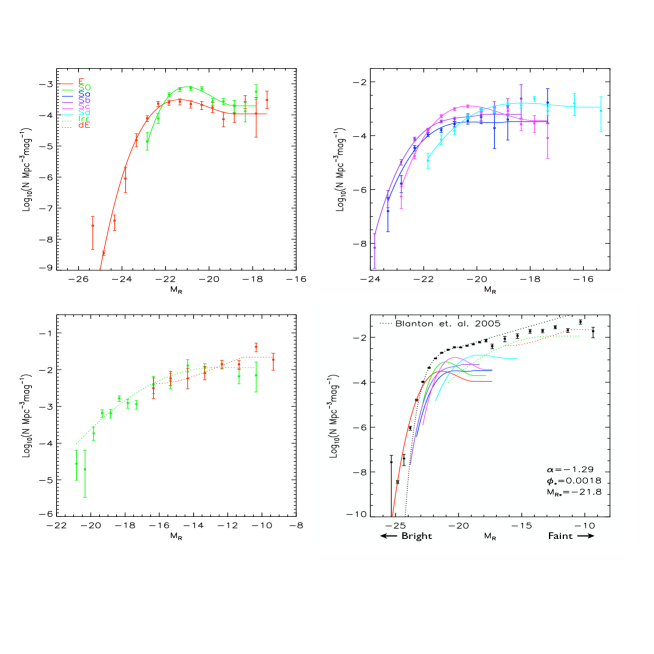
Figure 1: The field galaxy luminosity function split by Hubble Type. The top left plot is for Elliptical and S0 galaxies, the top right is for spirals (Sa-Sd), the bottom left is for the dwarf galaxies (irregular and elliptical) and the bottom right is the combined luminosity function. In each plot a spline-fit to the luminosity function is shown to guide the eye and these spline fits are also overlaid on the combined luminosity function in the bottom right plot. Galaxies which are very luminous in the R-band lie to left of these plots, while those which are very faint lie to the right. Overlaid on the bottom right panel are parameters for a Schechter fit to the total luminosity function.

The Hubble Type is a subjective assessment that depends on many parameters that can be measured for nearby bright galaxies. It cannot be determined for the faint galaxies in SDSS images, so we cannot determine type-specific luminosity functions from SDSS data alone. Broadband colours are often regarded as a straightforward way to distinguish between different kinds of galaxies. These are available for the SDSS sample, but this is a poor discriminant since different Hubble Types can have very similar colours (Fukugita et al. 1995), particularly different kinds of spiral galaxies. Another discriminant is the light concentration parameter, but this alone cannot be used to distinguish different types of late-type galaxies: concentration parameters do not depend on scale length if the profiles are exponential. H$\alpha$ emission-line strength is yet another discriminant, but there is considerable scatter in the H$\alpha$ equivalent width of galaxies of a single Hubble type (Kennicutt & Kent 1983).

We therefore use the following procedure: brightward of $M_{R}=-17.5$, concentration parameters, K-corrected broadband colours, and H$\alpha$ equivalent widths were used in conjunction with each other to classify the SDSS galaxies as early-type, intermediate-type, or late-type using local galaxies as templates. Luminosity functions were computed for each. The early-type luminosity function was then further split into an elliptical luminosity function and an S0 luminosity function in such a way that the relative numbers of these kinds of galaxies corresponded to that in each magnitude range in the Nearby Galaxies Catalogue (Tully 1988), which lists a sample of luminous galaxies within 40 Mpc. The intermediate luminosity function was split into a Sa luminosity function and a Sb luminosity function similarly. The late-type luminosity function was split into a Sc, a Sd, and an irregular luminosity function. Brightward of $M_{R}=-17.5$, dwarf elliptical galaxies do not seem to exist outside rich clusters (see e.g. Binggeli et al. 1988). Faintward of $M_{R}=-17.5$, the luminosity function was split according to the relative numbers of the different kinds of galaxies in the groups surveyed by Trentham & Tully (2002) and the Local Group.

This method of computing the luminosity function is motivated by our need to obtain stellar mass-to-light ratios and gas masses or galaxies of particular magnitudes and types. It forces the SDSS galaxy sample to have properties similar to the local galaxy sample, but it generates a luminosity function that is less susceptible to cosmic variance problems than a luminosity function derived from the local galaxy sample alone. Our method is subject to systematic problems if the two galaxy samples are very different. Other authors have used concentration parameters (see e.g. Kauffmann et al. 2003) or star formation histories derived from the SDSS spectra (Panter et al. 2004) to determine the mass-to-light ratios. Comparing our results to other values in the literature will be an important test of our method (see sections 3, 4 and 5).

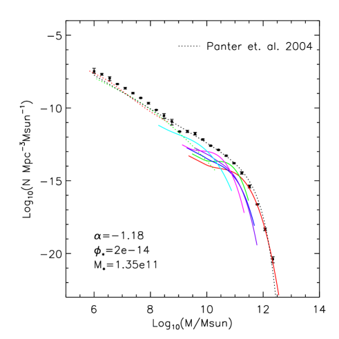
Figure 2: The field galaxy stellar mass function split by galaxy Hubble type. The data points are for all galaxies, while the lines show spine fits by Hubble Type. The lines have the same meaning as in Figure 1. Bright (massive galaxies) lie to the right of this plot, while faint galaxies lie to the left. Overlaid are parameters for a Schechter fit to the total mass function.

Our derived luminosity function agrees very well, both by Hubble type and integrated, with one obtained using only local galaxies (Binggeli et al., 1988). However, the agreement with a recent luminosity function obtained from the SDSS alone by Blanton et al. (2004) is not so good at the faint end (see dotted black line, Figure 1). Their faint end slope, corrected for incompleteness, is significantly steeper than ours (they find $\alpha\sim-1.5$; we find $\alpha\sim-1.3$). The difference could be caused by cosmic variance effects: our particular patch of the universe may be under-dense. In addition, Schechter fits to the bright end of the luminosity function (where the Poisson errors are small) tend to over-predict the number of faint galaxies.

Finally, notice that there is a dip in the luminosity function at $M_{R}\sim-17$. A similar dip in the luminosity function was recently found by Flint et al. (2003) suggesting that it might not simply be the result of incompleteness or poor overlap in the surveys used (see also Trentham et al. (2005) for further discussion of this feature).

3 The stellar mass function of field galaxies

In order to convert the luminosity function to a mass function, we require the mass-to-light ratio of the stellar populations. This will in general be a function of galaxy type, age, metallicity and even luminosity. We determine the mean mass-to-light ratio of ellipticals and assume that this may also be applied to the bulge component of S0 and spiral galaxies. We then determine the mean mass-to-light ratio of discs, irregular galaxies and dwarf elliptical galaxies. These mean mass-to-light ratios are then combined using bulge-to-disc ratios, $\mu_{B}$, using the measurements of Kent (1985). The results are presented, along with the gas properties of galaxies that we derive in the next section, in Table 1. In fact, we could do better than just taking a mean value for each of the Hubble types; in future work we will use a distribution of mass-to-light ratios as a function of luminosity for each Hubble type. This is beyond the scope of this present work.

$$\mu_{B}$$

E 1 6.8–7.5 1

S0+S0/a 0.64 4.8–5.4 0.11–0.33 1.3–6.7

Sa+Sab 0.33–0.40 3.1–3.6 0.078–0.32 1.5–5.8

Sb+Sbc 0.16–0.25 2.1–2.6 0.24–0.46 2.0–4.2

Sc+Scd 0.06–0.09 1.6–2.1 0.46–0.65 1.1–1.8

Sd+Sdm+Sm 0 1.6–2.1 0.62–0.70 0.70–1.3

Irr+dIrr 0 0.9–1.2 0.55–0.99 0.30–0.58

dE - 1.7–4.9 0 -

Table 2: Galaxy properties as a function of Hubble Type.

3.1 A note on random v.s. systematic errors

Stellar masses depend on both the galaxy luminosity function and the mass-to-light ratios of the stellar populations in the different kinds of galaxies. The errors in the former are random and are determined by counting statistics. The errors in the latter are systematic and come from our lack of knowledge about input parameters like metallicity and stellar IMF in the stellar population models used to calculate the mass-to-light ratios. We can get around this problem to some extent by comparing these mass-to-light ratios with those derived from dynamical measurements; we may then quote a range of mass-to-light ratios determined from these two methods. In this paper we take this pragmatic approach. However, the reader should be aware that dynamical measurements have their own systematic uncertainties and so it is not clear that we can really quantify all of our systematics in this way. As a conservative estimate, we suggest that the total systematic error may be as large as $\sim 50$% (compared with our quoted errors of $\sim 10$%). In future, we may hope to better quantify these systematics through spectroscopy of individual stars, deep photometry and improved modelling.

3.2 Ellipticals and bulges

Two methods were employed here. The first uses stellar population synthesis models to convert an age, metallicity and colour into a $B$-band mass-to-light ratio $M/L_{B}$. We use the models of Bruzual & Charlot (2003) with an initial stellar mass function (IMF), $\eta(M)$, taken from Kroupa (2001):

$$\eta(m)=\left\{\begin{array}[]{l@{\quad: \quad}l}25\,\eta(1)\,m^{-0.3}&0.01\leq m<0.08\\ 2\,\eta(1)\,m^{-1.3}&0.08\leq m<0.5\\ \,\eta(1)\,m^{-2.3}&0.5\leq m<100\end{array}\right.$$

(1)

where $m$ is in units of solar masses ${\rm M}_{\odot}$. The results are very sensitive to the IMF, since arbitrarily many low-mass stars can be included with no change to the measured colour, metallicity or age of a galaxy.

This IMF has been empirically determined from deep observations of local field stars and of young star clusters. It is denoted the ‘universal IMF’ since it appears to be the same across the enormous range of scale, environment and epoch in which it has been determined (Kroupa, 2001). This IMF is also attractive in that it is the end result of star formation that exhibits a Salpeter IMF whilst in progress (Kroupa & Weidner 2003).

Using the stellar population models of Bruzual & Charlot (2003), adopting the IMF above, and assuming a mean age and metallicity for ellipticals of $t_{E}\simeq 12\pm 2$ Gyr and $Z=2\,{\rm Z}_{\odot}$ respectively, we obtain $M/L_{B}=9.81-11.05$. Note that fitting a power law to the stellar population models of Bruzual & Charlot (2003) gives $M/L_{B}\sim 6.7({\rm Z}/{\rm Z}_{\odot})^{0.58}$. Thus the results are sensitive both to the choice of IMF, and to the choice of mean metallicity for the ellipticals.

We may also obtain the mass-to-light ratio of ellipticals from dynamics. While there is significant evidence for dark matter in ellipticals, interior to the majority of the stellar light the dark matter component is small (van der Marel 1991 and Kronawitter et al. 2000) so the stellar velocities (as measured from their relative Doppler shifts) may be used to calculate the total gravity produced by masses of the stars.

A recent study of 21 elliptical galaxies by Kronawitter et al. 2000 gives $M/L_{B}=6.78-7.54$ which is a factor $\sim 0.7$ of the stellar population value. This is surprising since the presence of dark matter should tend to make the stellar populations value smaller than the dynamical estimate rather than the other way round. We favour the dynamical estimate because modelling stellar populations is extremely difficult and errors of the order 2 are not uncommon (Charlot et al., 1996). Perhaps more importantly, the ‘universal’ IMF of Kroupa (2001) has not been explicitly verified for elliptical galaxies and so may not be the correct one to use (Jorgensen, 1997). Chabrier (2003) suggest an IMF which gives a much better agreement between stellar population models and dynamical masses for elliptical galaxies, however similar agreement may be obtained by using the Kroupa (2001) IMF and assuming a mean metallicity for ellipticals of solar, rather than twice solar. The double degeneracy of metallicity and IMF for the ellipticals leads us to favour the dynamical value for the mass to light ratio. This has its own systematic limitations: the internal velocity dispersions of ellipticals are unknown since only the line of sight velocities may be measured; and the presence of dark matter may complicate things at large radii. Future dynamical mass measurements, improved stellar population modelling, deep photometry of nearby galaxies and good spectra of individual stars will all help to pin down these systematic uncertainties in the future.

3.3 The mass-to-light ratio of discs

Following Fukugita et al. (1998) we compile a mean mass-to-light ratio for discs from three independent methods. The first is from measurements of the column density of stars in the solar neighbourhood, $\Sigma_{*}=27-40$M_⊙pc^-2 (Gould et al. 1996 and Kuijken & Gilmore 1989). Combining this with the local luminosity surface density, $\Sigma_{L_{B}}\simeq 18$M_⊙pc^-2 (Bahcall & Soneira, 1980) gives $M/L_{B}=1.5-2.2$. The second method uses the stellar population synthesis models of Tinsley (1981) and Portinari et al. (2004). These are on a firmer footing than for the elliptical galaxies since the IMF has been explicitly measured for spiral galaxies (Kroupa, 2001). These give $M/L_{B}=1.1-1.9$ using the IMF given in equation 1. The third method uses a dynamical mass estimate for the stars (Salucci & Persic 1999). This gives $M/L_{B}=1.11$.

The mean of all of these values gives $M/L_{B}=1.24-1.7$. We adopt this value here. This value was then corrected for internal extinction in the galaxies, using the corrections of (Tully & Fouque, 1985) and a field sample inclination distribution equivalent to that seen in the Ursa Major Cluster (Tully et al., 1996). A similar value for $M/L_{B}$ was recently obtained dynamically from a compilation of spiral galaxies by McGaugh (2004). This further strengthens our confidence in this value.

3.4 The mass-to-light ratio of dwarfs and irregulars

The mass-to-light ratios for the irregulars (and dwarf irregulars) may be adapted from the above value for discs corrected for their younger age and consequent bluer colour (Fukugita et al., 1998): $M/L_{B}=0.9-1.24$.

Recent observations of the Ursa Minor Local Group dwarf elliptical (dE) galaxy by Wyse et al. (2002) suggest that dE stellar populations are very similar to the Milky Way globular clusters. As such, we use the dynamical mass-to-light ratio of Galactic globular clusters (Pryor & Meylan 1993) for dE galaxies: $M/L_{B}=1.7-4.9$.

We find excellent agreement between our derived stellar mass function and that of Panter et al. (2004) (see the black dotted line in Figure 2). They also use the SDSS data, but derived stellar masses from star formation histories constrained by the spectra of the galaxies. This gives some weight to the validity of our method of classifying galaxies by Hubble type and then determining masses. Our data gives $\Omega_{*}=0.0028\pm 0.0003$, whereas Panter et al. find $\Omega_{*}=0.0034\pm 0.0001$.

4 The gas mass function of field galaxies

The gas mass function of local galaxies is presented in Figure 3.

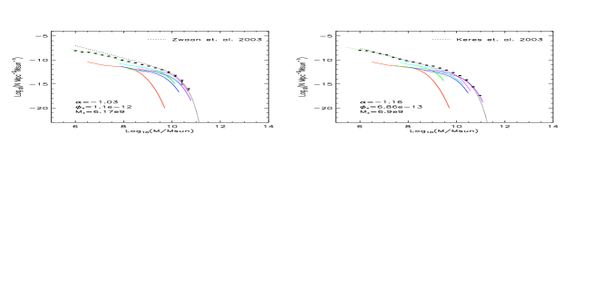
Figure 3: The field galaxy HI (left) and H₂ (right) gas mass functions split by galaxy Hubble Type. The data points are for all galaxies, while the lines show spine fits by Hubble type. The lines are as in Figure 1. Overlaid are parameters for a Schechter fit to the total mass function.

4.1 Atomic hydrogen (HI)

A large sample of HI (atomic) gas measurements of nearby galaxies was compiled recently as part of the Australian HIPASS survey, using the Parkes radio telescope. Measurements of the 1000 brightest galaxies in this sample were recently published (Koribalski et al. 2004).

In order to measure the total amount of gas in galaxies in the Universe, we need to determine how much gas the galaxies contain per unit optical luminosity. We can then get the gas mass function from the luminosity function. We computed the atomic gas mass per unit luminosity for each Hubble Type as follows. We compiled a sample of galaxies with velocities between 2000 and 3000 km/s that were observed at optical wavelengths and also in HI in the HIPASS survey. For each Hubble Type, we used this sample to determine the ratio between the atomic gas mass and the optical luminosity. These numbers are given in Table 2. The wide ranges reflect the conservative error estimates that we are forced to use because of the intrinsic scatter in the ratio for galaxies of a given Hubble Type and because the errors are systematic (see also section 33.1).

The HI mass function that we derived is very similar to the one derived by HIPASS (Zwaan et al. 2003) at the high-mass end, but falls significantly below theirs at the low-mass end. This difference can be attributed to the difference in sample selection and scaling – the HIPASS sample is selected by HI mass but ours is selected and scaled by optical luminosity. They therefore include many systems that we do not, as well as including gas in the outer parts of galaxies which is not included in our analysis – a galaxy that we think has mass $M$ of atomic gas may really have $2M$, so our points should be shifted towards the right if we wish to include all the atomic gas in the Universe. Both of these effects could be more important at low masses – the highest mass HI galaxies will invariably be in optical surveys, and all scaling relations were derived using the properties of these galaxies.. This difference also accounts in our different values of $\Omega_{\rm HI}$: HIPASS finds $\Omega_{\rm HI}=(4.1\pm 0.6)\times 10^{-4}$, whereas we get $\Omega_{\rm HI}=(2.9\pm 0.6)\times 10^{-4}$.

4.2 Molecular hydrogen (H₂)

Similarly, we determine the relationship between galaxy Hubble Type and molecular gas mass using the data of Young et al. (1995). The results are also presented in Table 2. This survey measures CO line luminosities, which are converted to gas masses using the empirical formula of Young & Scoville (1991): $M_{\rm H_{2}}=12000\,S_{\rm CO}D^{2}{\rm M}_{\odot}$, where $S_{\rm CO}$ is the CO flux in Jy km/s and $D$ is the distance to the galaxy in Mpc.

We find a very similar molecular gas mass function to that of Keres et al. (2003), who presented this function for a far-infrared (FIR)-selected sample, also derived from the Young et al. (1995) sample. This is consistent with the idea that most of the currently observed molecular gas in the Universe is in normal galaxies, which are the same objects as the FIR sources.

5 The baryonic mass function of field galaxies

The baryonic mass function is presented in Figure 4. This is the sum of the functions in the three previous Figures, where the masses in the gas functions are multiplied by 1.33 to take into account the presence of helium. The error bars are small enough that Schechter or any other analytical fits to the data are formally poor. However, we show our best fit values on the plot.

In Table 3, we present the total mass density of the Universe in baryons within galaxies, in different forms. Typical errors are 10% (but see section 33.1). For the stellar masses the uncertainty mainly comes from our lack of knowledge of the mass-to-light ratios. For the gas components the error primarily comes from the uncertainty in the scaling of optical luminosity to gas mass for galaxies of a given Hubble Type.

About 8% of the baryons in galaxies are in atomic gas and about 7% are in molecular gas. In the Milky Way about 8% of the baryons are in atomic gas and a further 2% are in molecular gas.

A comparison with the CDM mass function is also shown in Figure 4. The normalisation for the baryonic component in galaxies is very much lower, reflecting the fact that galaxy masses are dominated by dark matter, not baryons. Additionally, the baryonic mass function has a very different shape from the dark mass function. This suggests that the collapse of baryons into galaxies and the ability of the galaxies to retain the gas once star formation has begun is very much a scale-dependent process. At the very low mass end, where galaxies are heavily dark-matter dominated, the baryonic mass function is still very much shallower than the CDM mass function – this is the classical missing satellites problem (Moore et al., 1999). At the high mass end it is also deficient. This could be caused by feedback from centrally active black holes within galaxies (Silk & Rees, 1998).

Finally, notice that there is a slight bump in the baryonic mass function at $\sim 10^{9}$M_⊙. This corresponds to a similar dip in the stellar mass function (see Figure 2) and a dip in the luminosity function at $M_{R}\sim-17$ (see Figure 1 and section 2). The dip is much less significant in the baryonic mass function than in the stellar mass function and the luminosity function. It is possible in all cases that this dip is a statistical artifact: its significance is not high. However it is interesting that it occurs at the transition point in galaxy type from ellipticals and spirals to dwarfs. The fact that it is less pronounced in the full baryonic mass function than in the stellar mass function may then simply highlight the fact that the gas mass fraction in dwarf irregulars is much larger than in ellipticals and spirals.

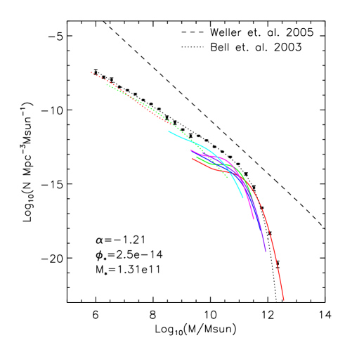
Figure 4: The field galaxy baryonic mass function. The data points are for all galaxies, while the lines show spine fits by Hubble Type. The lines are as in Figure 2. The CDM mass spectrum from the numerical simulations of Weller et al. (2004) is also shown. Overlaid are parameters for a Schechter fit to the total mass function.

	$\Omega_{b}$	$\Omega_{*}$	$\Omega_{HI}$	$\Omega_{H_{2}}$
E	0.00064	0.00064	$\sim 0$	$\sim 0$
S0	0.00073	0.00068	0.00003	0.00001
Sa+Sab	0.00036	0.00032	0.00001	0.00002
Sb+Sbc	0.00056	0.00040	0.00004	0.00008
Sc+Scd	0.00072	0.00047	0.00010	0.00008
Sd+Sdm+Sm	0.00037	0.00021	0.00007	0.00005
Irr+dIrr	0.00013	0.00007	0.00003	0.00001
dE	0.00002	0.00002	$\sim 0$	$\sim 0$
total	0.0035	0.0028	0.00029	0.00026

Table 3: The baryonic mass density of galaxies. Typical errors are $\sim 10$%. A discussion of the larger systematic errors is given in section 33.1.

There are a number of baryonic mass components which we have not included in the above analysis because they comprise only a tiny fraction of the total mass in baryons within galaxies.

Field halo stars: In the Milky Way and M31 there is a faint spheroidal stellar population of stars which lie neither in the disc nor bulge components of the galaxy (Gilmore et al., 1989). While the total mass of this component is quite uncertain and estimates range from $\sim 10^{8}$ (Binney & Merrifield, 1998) to $\sim 10^{9}$ M_⊙ (Freeman & Bland-Hawthorn, 2002), this is still only $\sim 0.1-1$% of the total baryonic mass and, therefore, a negligible Galactic mass component. Because of the low surface density of these halo stars, they are difficult to resolve in galaxies much further away than M31. Perhaps other galaxies have a much more significant stellar halo and we are missing an important baryonic mass component. This is probably not the case, however, because stars from these halos would generate a high extragalactic background light in galaxy clusters, which is not observed (Zibetti et al., 2005).

MACHOs and stellar remnants: Limits can be placed on massive compact halo objects (MACHOs) of any form, which may or may not be made of baryonic matter, from microlensing experiments (e.g. Alcock et al. 2000). Current data (Afonso et al. 2003) suggests that the contribution of MACHOs to the total baryonic mass of the Galaxy may be small, and we neglect this contribution here. A more stringent constraint can be placed on the total mass in MACHOs that are the endpoints of stellar evolution (neutron stars and black holes) due to the lack of large amounts of heavy elements in the Universe (e.g. Freese et al. 2001). Fukugita & Peebles (2004) estimated the cosmological density in the remnants to be $\Omega_{\rm remnants}\sim 0.00001$, which is far less than the sums in Table 3, and we ignore this contribution here.

Hot gas: There are two main hot ionised gas components in galaxies: a component associated with HII regions, which is heated by ionising radiation from O and B stars, and an extended component which is associated with the dark matter halo. The mass of the component associated with HII regions is negligible ($\sim$ a tenth of the molecular gas mass) for both early and late type galaxies (e.g. O’Sullivan et al. 2001, Mathews & Brighenti 2003 and Goudfrooij 1999). The extended component is what we refer to later as the warm/hot intergalactic medium or WHIM. Some of this gas is likely bound to galaxies; much of it presumably also resides in the intergalactic medium. This component, which we do not count as part of galactic baryonic matter, is probably the dominant form of baryons in the Universe.

Dust: In the Milky Way, a dust-to-gas ratio by mass is about 1/200 (Gilmore et al., 1989). There does not seem to be any evidence for this ratio being different in the majority of external normal galaxies (see e.g. the review by Young and Scoville 1991), and we neglect the contribution of dust to the baryonic mass density of the Universe.

6 The contribution to $\Omega_{b}$

The value that we get of $\Omega_{\rm b,gal}\sim 0.0035$ in galaxies is only about one-tenth of the value of the baryonic density of the universe $\Omega_{\rm b}\sim 0.05$ derived from measurements of light element abundances (Coc et al. 2004) and from the shape of the angular power spectrum of the cosmic microwave background (Spergel et al., 2003). This opens up the important question: if they are not in galaxies, where do 90% of the baryons in the Universe reside?

Hydrodynamic simulations (Cen & Ostriker 1991) suggest that most of these baryons are in a warm/hot intergalactic medium (WHIM), that is highly ionised. This medium is very difficult to detect, but there might be indirect evidence for its existence, from observations of OVII X-ray absorption along the lines of sight to high redshift quasars (e.g. Fang et al. 2003). Directly detecting the WHIM and will be a major area of observational study over the next few years.

7 Conclusions

The main conclusions from this work are as follows:

1. The baryonic density of the universe that resides in galaxies is $\Omega_{\rm b,gal}=0.0035\pm 0.0003$. This is far less than the value of $\Omega_{\rm b}=0.05$ inferred from the CMB or from BBN. Most of the baryons in the Universe do not reside in galaxies and probably reside in the warm/hot intergalactic medium (WHIM). Direct detection of the WHIM will form one of the major challenges for astronomy in the next decade.

2. Most of the baryons in galaxies are in stars, not gas, and about one-half of these stars are in early-type galaxies. We derive the value of $\Omega_{*}=0.0028\pm 0.0003$, assuming stellar mass-to-light ratios derived from population synthesis models, a Kroupa IMF in discs and irregular galaxies and stellar mass-to-light ratios derived from dynamical measurements in bulges and elliptical galaxies.

3. About 15–20% of the baryons in galaxies are in gas. Of this, about one half is in molecular gas.

4. About 30% of the atomic gas seen by HIPASS is not present in our atomic gas mass function. We attribute this to gas in galaxies that are missing in the sample that we used to define a scaling between optical luminosities and gas masses.

The main uncertainties in this work arise from the systematic errors in determinations of the stellar and gas mass-to-light ratios. The errors we quote throughout this paper are small, since they derive from the range in mass-to-light ratios determined from different methods. Such errors do not take account of systematic errors within each mass determination which are much harder to quantify and may be as large as 50%. Spectroscopy, deep photometry and improved modelling will all help to pin down and reduce such systematics in the future. An accurate baryonic mass function is already beginning to form one of the observational pillars of modern cosmology.

8 Acknowledgements

We would like to thank the three anonymous referees, Stacy McGaugh and Gilles Chabrier for their useful comments.

References

- Abazajian et al. (2004) Abazajian et al. 2004, AJ, 128, 502
- Afonso et al. (2003) Afonso et al. 2003, A&A, 404, 145
- Alcock et al. (2000) Alcock et al. 2000, ApJ, 541, 734
- Allen et al. (2004) Allen et al. 2004, MNRAS, 353, 457
- Bahcall & Soneira (1980) Bahcall J. N., Soneira R. M., 1980, ApJS, 44, 73
- Bell et al. (2003) Bell E. F., McIntosh D. H., Katz N., Weinberg M. D., 2003, ApJ, 585, L117
- Bertschinger (1998) Bertschinger E., 1998, ARA&A, 36, 599
- Binggeli et al. (1988) Binggeli B., Sandage A., Tammann G. A., 1988, ARA&A, 26, 509
- Binney & Merrifield (1998) Binney J., Merrifield M., 1998, Galactic astronomy. Princeton University Press.
- Blanton et al. (2004) Blanton M. R., et al., 2004
- Borriello & Salucci (2001) Borriello A., Salucci P., 2001, MNRAS, 323, 285
- Bruzual & Charlot (2003) Bruzual G., Charlot S., 2003, MNRAS, 344, 1000
- Cen & Ostriker (1999) Cen R., Ostriker J. P., 1999, ApJ, 514, 1
- Chabrier (2003) Chabrier G., 2003, PASP, 115, 763
- Charlot et al. (1996) Charlot S., Worthey G., Bressan A., 1996, ApJ, 457, 625
- Coc et al. (2004) Coc et al. 2004, ApJ, 600, 544
- Cole et al. (2001) Cole et al. 2001, MNRAS, 326, 255
- Colless et al. (2001) Colless et al. 2001, MNRAS, 328, 1039
- Davé et al. (2001) Davé R., Cen R., Ostriker J. P., Bryan G. L., Hernquist L., Katz N., Weinberg D. H., Norman M. L., O’Shea B., 2001, ApJ, 552, 473
- de Blok et al. (2001) de Blok W. J. G., McGaugh S. S., Bosma A., Rubin V. C., 2001, ApJ, 552, L23
- Derue et al. (2001) Derue et al. 2001, A&A, 373, 126
- Fang et al. (2003) Fang T., Sembach K. R., Canizares C. R., 2003, ApJ, 586, L49
- Flint et al. (2003) Flint K., Bolte M., Mendes de Oliveira C., 2003, Ap&SS, 285, 191
- Freeman & Bland-Hawthorn (2002) Freeman K., Bland-Hawthorn J., 2002, ARA&A, 40, 487
- Freese et al. (2001) Freese K., Fields B. D., Graff D. S., 2001, in Identification of Dark Matter . p. 213
- Frei & Gunn (1994) Frei Z., Gunn J. E., 1994, AJ, 108, 1476
- Fukugita et al. (1998) Fukugita M., Hogan C. J., Peebles P. J. E., 1998, ApJ, 503, 518
- Fukugita & Peebles (2004) Fukugita M., Peebles P. J. E., 2004, ApJ, 616, 643
- Fukugita et al. (1995) Fukugita M., Shimasaku K., Ichikawa T., 1995, PASP, 107, 945
- Gao et al. (2004) Gao J., Chen L., Wang J., Hou J., Zhao J., 2004, Progress in Astronomy, 22, 275
- Gilmore et al. (1989) Gilmore G., Wyse R. F. G., Kuijken K., 1989, ARA&A, 27, 555
- Goudfrooij (1999) Goudfrooij P., 1999, in Ast. Soc. of the Pacific Conf. Series . p. 55
- Gould et al. (1996) Gould A., Bahcall J. N., Flynn C., 1996, ApJ, 465, 759
- Jorgensen (1997) Jorgensen I., 1997, MNRAS, 288, 161
- Kauffmann et al. (2003) Kauffmann et al. 2003, MNRAS, 341, 33
- Kennicutt & Kent (1983) Kennicutt R. C., Kent S. M., 1983, AJ, 88, 1094
- Kent (1985) Kent S. M., 1985, ApJS, 59, 115
- Keres et al. (2003) Keres D., Yun M. S., Young J. S., 2003, ApJ, 582, 659
- Kleyna et al. (2001) Kleyna J. T., Wilkinson M. I., Evans N. W., Gilmore G., 2001, ApJ, 563, L115
- Koribalski et al. (2004) Koribalski et al. 2004, AJ, 128, 16
- Kronawitter et al. (2000) Kronawitter A., Saglia R. P., Gerhard O., Bender R., 2000, A&AS, 144, 53
- Kroupa (2001) Kroupa P., 2001, MNRAS, 322, 231
- Kroupa & Weidner (2003) Kroupa P., Weidner C., 2003, ApJ, 598, 1076
- Kuijken & Gilmore (1989) Kuijken K., Gilmore G., 1989, MNRAS, 239, 605
- Mathews & Brighenti (2003) Mathews W. G., Brighenti F., 2003, ARA&A, 41, 191
- Mayer (2004) Mayer L., 2004, in Proc. of Baryons in Dark Matter Halos. . p. 37
- McGaugh (2004) McGaugh S. S., 2004, ApJ, 609, 652
- Mellier (1999) Mellier Y., 1999, ARA&A, 37, 127
- Moore et al. (1999) Moore B., Ghigna S., Governato F., Lake G., Quinn T., Stadel J., Tozzi P., 1999, ApJ, 524, L19
- Nagamine et al. (2005) Nagamine K., Cen R., Hernquist L., Ostriker J. P., Springel V., 2005, ApJ, 618, 23
- O’Sullivan et al. (2001) O’Sullivan E., Forbes D. A., Ponman T. J., 2001, MNRAS, 328, 461
- Panter et al. (2004) Panter B., Heavens A. F., Jimenez R., 2004, MNRAS, 355, 764
- Peacock (1999) Peacock J. A., 1999, Cosmological physics. Cosmological physics. Publisher: Cambridge, UK: Cambridge University Press, 1999. ISBN: 0521422701
- Portinari et al. (2004) Portinari L., Sommer-Larsen J., Tantalo R., 2004, MNRAS, 347, 691
- Pryor & Meylan (1993) Pryor C., Meylan G., 1993, in Ast. Soc. of the Pacific Conf. Series . p. 357
- Riess et al. (2004) Riess et al. 2004, ApJ, 607, 665
- Salucci & Persic (1999) Salucci P., Persic M., 1999, MNRAS, 309, 923
- Sand et al. (2004) Sand D. J., Treu T., Smith G. P., Ellis R. S., 2004, ApJ, 604, 88
- Schechter (1976) Schechter P., 1976, ApJ, 203, 297
- Silk & Rees (1998) Silk J., Rees M. J., 1998, A&A, 331, L1
- Spergel et al. (2003) Spergel et al. 2003, ApJS, 148, 175
- Springel et al. (2005) Springel V., White S. D. M., Jenkins A., Frenk C. S., Yoshida N., Gao L., Navarro J., Thacker R., Croton D., Helly J., Peacock J. A., Cole S., Thomas P., Couchman H., Evrard A., Colberg J., Pearce F., 2005, Nature, 435, 629
- Springob (2004) Springob C. M., 2004, American Astronomical Society Meeting Abstracts, 205,
- Tinsley (1981) Tinsley B. M., 1981, ApJ, 250, 758
- Trentham et al. (2005) Trentham N., Sampson L., Banerji M., 2005, MNRAS, pp 52–+
- Trentham & Tully (2002) Trentham N., Tully R. B., 2002, MNRAS, 335, 712
- Tully (1988) Tully R. B., 1988, Nearby galaxies catalog. Cambridge University Press
- Tully & Fouque (1985) Tully R. B., Fouque P., 1985, ApJS, 58, 67
- Tully et al. (1996) Tully et al. 1996, AJ, 112, 2471
- van der Marel (1991) van der Marel R. P., 1991, MNRAS, 253, 710
- Weller et al. (2004) Weller J., Ostriker J. P., Bode P., 2004
- Wyse et al. (2002) Wyse et al. 2002, New Astronomy, 7, 395
- Young & Scoville (1991) Young J. S., Scoville N. Z., 1991, ARA&A, 29, 581
- Young et al. (1995) Young et al. 1995, ApJS, 98, 219
- Zibetti et al. (2005) Zibetti S., White S. D. M., Schneider D. P., Brinkmann J., 2005