Far-Infrared and Millimeter Continuum Studies of K Giants: $\alpha$ Boo and $\alpha$ Tau

Abstract

We have imaged two normal, non-coronal, infrared-bright K giants, $\alpha$ Tau and $\alpha$ Boo, in the 1.4-mm and 2.8-mm continuum using BIMA. These stars have been used as important absolute calibrators for several infrared (IR) satellites. Our goals are: (1) to establish whether these stars radiate as simple photospheres or possess long-wavelength chromospheres; and (2) to make a connection between millimeter-wave and far-infrared (FIR) absolute flux calibrations. To accomplish these goals we also present ISO Long Wavelength Spectrometer (LWS) measurements of both these K giants. The FIR and millimeter continuum radiation is produced in the vicinity of the temperature minimum in $\alpha$ Tau and $\alpha$ Boo. We find that current photospheric models predict fluxes in reasonable agreement with those observed for wavelengths which sample the upper photosphere, namely $\leq$125 $\mu$m in $\alpha$ Tau and $\alpha$ Boo. We clearly detect chromospheric radiation from both stars by 2.8 mm (by 1.4 mm in the case of $\alpha$ Boo). Only additional observations can determine precisely where beyond 125 $\mu$m the purely radiative models fail. Until then, purely radiative models for these stars can only be used with confidence for calibration purposes below 125 $\mu$m.

1 Introduction

We had two distinct objectives in undertaking this work, dominantly to investigate the merit and reliability of K giant stars as absolute FIR and millimeter calibration sources, but secondarily to determine just how shallow in depth simple radiative equilibrium cool star model atmospheres might be trusted.

We have chosen $\alpha$ Tau and $\alpha$ Boo for this initial study because these stars, being both bright and nearby, are easily the two most completely and thoroughly studied red giants. This makes them the ideal test cases for our purposes. It should be noted that they both lie on the cool, non-coronal side of the “Linsky-Haisch dividing line” (Linsky & Haisch, 1979) which separates coronal from non-coronal giants, although Ayres et al. (1997) have found evidence for buried high temperature emission in the case of $\alpha$ Boo.

1.1 Infrared calibration stars

Cohen and colleagues have presented a self-consistent context for absolute calibration in the IR, ideal for use by ground-based, airborne, and spaceborne spectrometers and radiometers (Cohen et al., 1992a, b, c, 1995; Cohen & Davies, 1995; Cohen et al., 1996a, b, 1999). Their approach is based upon a pair of absolutely calibrated, IR-customized models of Vega and Sirius calculated by Kurucz. These efforts have furnished the absolute stellar spectrum of Sirius that underpins COBE/DIRBE bands $1-5$ (Mitchell et al., 1996; Cohen, 1998), the spectra of K0-M0IIIs for the on-orbit calibration of the Near- and Mid-Infrared Spectrometers on the joint NASA/ISAS Infrared Telescope in Space (Murakami et al., 1997), likewise for ESA’s Infrared Space Observatory (ISO) (Kessler et al., 1996) instruments (e.g., the Short Wavelength Spectrometer) (Schaeidt et al., 1996), for the Spatial InfraRed Imaging Telescope (SPIRIT-III) on the US Midcourse Space Experiment (MSX) (Mill et al., 1994), and for 2MASS (Cohen et al., 2003b). An extension of this work to substantially fainter stars has provided calibrators for the Spitzer Space Telescope (Cohen et al., 2003a). Most recently, Price et al. (2004) have absolutely validated the two calibrated model spectra, and the empirical spectra of the brighter K giants such as $\alpha$ Tau and $\alpha$ Boo, in six bands in the mid-infrared (MIR), using precision measurements from the MSX.

The absolute calibration of ISOPHOT (Lemke et al., 1996; Schulz et al., 2002) was supported by planets, asteroids, and stars, ranked in order of decreasing flux density (Muller & Lagerros, 1998; Schulz et al., 2002). The stellar calibrators (Cohen et al., 1996b) necessitated long-wavelength extrapolations, as far as 300 $\mu$m, of the observed (1.2–35 $\mu$m) absolute stellar spectra by model atmosphere spectra (computed by one of us [DFC]: Cohen et al. (1996b)). We note that the bright, secondary reference stars that have been selected for IR calibration purposes are precisely those “quiet” giants in which it was suggested that radiatively-cooled regions very largely dominate the stellar surfaces so that single component atmospheric models were most likely to be valid. Examples of these are $\alpha$ Boo, $\alpha$ Hya, $\alpha$ Tau, and $\gamma$ Dra (Wiedemann et al., 1994). Consequently, one of our objectives is to establish whether these stars radiate as predicted, thereby validating the scheme used for ISO at the longest wavelengths, or possess long-wavelength chromospheres.

1.2 Linking infrared and millimetric calibration

The ISO Long Wavelength Spectrometer (LWS) (Clegg et al., 1996; Swinyard et al., 1996) used Uranus as a calibration standard but also observed Neptune, and Mars when it became available. Although Uranus has remained the LWS primary calibrator, the Mars spectrum has been shown to be fully consistent with this Uranus framework (Sidher et al., 2003). In the case of Neptune, a new model based on the LWS data has been adopted (Orton et al., 2000). LWS was able to observe some stellar calibrators (Lim et al., 1997), although these observations were difficult to make due to poor signal-to-noise in the relatively narrow LWS bandwidths. However, the stellar spectra did demonstrate consistency with the Uranus-Mars framework, in the LWS 45–170 $\mu$m region. In this paper we present the totality of results from the ISO LWS spectra obtained on $\alpha$ Tau and $\alpha$ Boo.

The long-wavelength stellar spectral extrapolations are based upon the assumption that these calibrator stars are not attended by extensive chromospheres. Radiometric testing with ISOPHOT (Muller & Lagerros, 1998; Schulz et al., 2002) suggests that these extrapolations were meaningful, i.e. consistent with calibrations based on asteroids and planets. It would be of great interest, both scientific and pragmatic, to determine independently whether these same stellar calibrators radiate as predicted in the millimeter (mm) domain. The basis for mm-wave absolute flux calibration is Mars. Therefore, we observed the stellar calibrators against Mars, or against secondary microwave standards that were ultimately traceable to a comparison with Mars, Uranus, or Neptune. By this means we hoped to provide a link between the reference flux density scales of planets and stars and to unify flux calibration across the IR-mm regime. Early efforts in this direction at Berkeley were described by Wrixon et al. (1971). Gibson et al. (2005) and Welch & Gibson (2005) have continued this radio absolute calibration work.

1.3 Cool stellar atmospheres

Our secondary goal is to probe the structure of the outer atmospheres in K and, eventually, M giants. Vernazza et al. (1976) demonstrated in a classic paper how observations of the solar FIR continua, atomic lines, and UV continua could be brought together to construct a single-component, time-independent mean solar temperature structure. FIR continuum fluxes were of crucial importance in helping to establish this mean structure from the upper photosphere, through the temperature minimum region, and into the chromosphere. Using the FIR continuum to probe the shallow depths in solar and cooler stars is possible because the primary IR continuous opacity, H^- free-free, increases as $\lambda^{2}$, pushing the depth of continuum formation into the outermost stellar layers. Until now these layers in cool stars have been accessible only through non-LTE analyses of the cores of strong atomic and molecular lines (e.g., Ayres & Linsky (1975), Kelch et al. (1978), McMurry (1999), Wiedemann et al. (1994)).

While chromospheric models have become more complex in the years since the Vernazza et al. (1976) study, the FIR and millimeter fluxes still have the potential to be valuable diagnostics of the shallow stellar layers. In accurately determining the FIR and millimeter fluxes of selected red giants, we hope to provide useful information for testing models of the cool star stellar photospheres and chromospheres. We are particularly interested in determining the location of the transition from observed fluxes, reproducible by purely radiative equilibrium models, to fluxes that require invoking a non-radiatively heated chromosphere. In addition, we wish to trace the observed run of decreasing fluxes with increasing wavelength from the upper photosphere and determine how closely current stellar model atmosphere calculations can match this run. This information on the location of the temperature reversal and the quality of fit to the fluxes originating in the upper photosphere are vital in defining the wavelength range for which simple radiative models may be used for FIR calibrations.

2 The observations

Table 1 summarizes our various sets of mm observations, listing array configurations and frequencies used, integration times on the stars, phase and flux calibrators (chosen to be as close to each star’s direction in the sky as possible), and the primary or secondary mm-calibrator observed with each set of stellar observations. A few measurements were taken in the B-array, with which planetary calibrators like Mars were partially resolved, necessitating an extra step in the calibration process to calculate the flux expected on the shortest baseline pairs (see below). Consequently, we preferred measurements in C- or D-array configurations. Angular diameters of these stars in the optical to MIR regions are of order 20 mas, rendering them unresolved targets in all these configurations, as were the local calibrators chosen. On the basis of estimates of the BIMA performance at 1 and 3 mm, our observing scripts called for typical tracks of several hours’ duration, of which between roughly two and four hours were spent on the stars themselves.

This was a continuum experiment, and we selected observing frequencies from considerations of the expected stellar spectra, receiver performance, and atmospheric transmission. Whenever possible we included measurements of Mars with each set of stellar and local calibration source observations, in an attempt to unify the calibration. For those few data sets taken in an array configuration that resolved Mars, we calculated visibilities as a function of baseline (in kilo$\lambda$) and applied these partial-resolution factors to the Mars model (Wright, 1976) flux densities using our shortest baseline pairs.

Sometimes no planet was visible close in time to our observing tracks. Then we used MWC 349 when it was available. Hat Creek has a long series of observations of this star, it is relatively bright, has shown no statistically significant variability in our archives, and has been modeled in detail by Dreher & Welch (1983) so that flux extrapolation and interpolation to our frequencies is viable. Further, Welch & Gibson (2005) have obtained its mm flux densities to a precision of 1% absolute. For our final observations, in December 2000, we used W3OH as reference for our $\alpha$ Tau track, again because of its relative proximity to this star, long-term temporal stability of signal, and the available multifrequency Hat Creek archives which enable interpolation between known flux densities at other frequencies to our own. We treated W3OH as having a canonical Hii region spectrum and included the frequency dependence of the Gaunt factor. Other secondary references such as 1415+133 and 0530+135 were likewise observed when no other obvious flux reference presented itself. Independent observations of these were extracted from the Hat Creek archives, preferably with respect to a primary or acceptable secondary standard. In such circumstances, Table 1 carries the primary standard to which the flux pedigree of such a secondary is traceable.

Upper and lower sidebands were processed independently, maps made of the stars at each frequency, and peak flux densities extracted (see the final column of Table 1). Sometimes, weather conditions were adequate in the lower sideband but led to unacceptably large noise in the upper sideband. In such cases we eliminated the noisy datasets which were readily recognized by the presence of artifacts in the maps, such as global striping, or large negative-going blobs. To estimate the uncertainties in the tabulated peak flux densities derived from any map, we used the standard deviation calculated from substantial regions of the map that excluded the target star itself. To combine the simultaneous upper and lower sideband maps at one epoch, we used inverse-variance weighting of the two maps based upon these noise estimators, relying upon the miriad task maths. Likewise, we combined results across epochs.

3 Self-calibration of the 1-mm data

Phase calibration of interferometer data relies on transferring phases accurately from a point source (usually a QSO) to the target source. The accuracy of the calibration depends on the distance between source and calibrator, baseline errors, atmospheric phase stability, and the signal-to-noise ratio (SNR) in the phase measurement of the calibrator. All sources of phase error result in decorrelation of the calibrated image; i.e., a lower amplitude in the final map compared with perfectly calibrated data. Self-calibration offers a way to eliminate these phase errors, but is limited by the timescale on which phase can be accurately measured on the target source itself.

In the case of $\alpha$ Boo, the measured peak flux density in the normally calibrated image is about 50 mJy. Given the system temperature (350 K), bandwidth (670 MHz, reduced from 800 MHz due to edge-channel flagging in the wideband average), and a correlator efficiency of 0.88 (2-bit) for these observations, the expected noise in a single-interferometer measurement is about 70 mJy in 10 min. Using self-calibration with a 9-element array improves the SNR for antenna-based phases by about a factor of 3, due to baseline averaging. The expected r.m.s. noise in the antenna-based phases using self-calibration is, therefore, about 25 mJy in 10 min. Assuming the true flux of $\alpha$ Boo to be 80 mJy, we would expect an SNR of about 3 using 10-min averaging on the source. The expected phase error for an SNR of 3 is $\sim 20^{\circ}$ for each antenna (arcsin(1/3)). The decorrelation expected for an r.m.s. phase error of 20^∘ is about 6% (reduced amplitude = exp($-r^{2}/2$), where $r$=the r.m.s. phase error in radians). It would, therefore, appear safe to use an interval of 10 min or longer to self-calibrate the 1-mm $\alpha$ Boo data in phase. Of course, any additional phase error (e.g., atmospheric) incurred during the self-calibration interval will increase the decorrelation in the final image.

We can estimate the amount of atmospheric decorrelation expected. The average r.m.s. delay path in 10 min for a 100 m baseline on the day of the $\alpha$ Boo 1-mm observations (01 Jun 2000) was 210 $\mu$m, or $\sim$1 rad at 1360 $\mu$m wavelength. In D-array, the maximum baseline is about 30 m. Assuming that the atmospheric r.m.s. phase scales as (baseline)^5/6, the r.m.s. phase becomes 0.37 rad on the longest baseline [(30 m/100 m)^5/6 * 1 rad], and about 0.2 rad for the median baseline of 15 m. The expected atmospheric decorrelation in 10 min for the 30 m baseline ($r$=0.37 rad) is 0.85, and for the 15 m baseline ($r$=0.2 rad) is 0.98. Thus, atmospheric decorrelation on 10-min timescales is not expected to be very important, and phase variations on the longer timescales will be removed by the self-calibration.

We validated these ideas on the June 2000 observations of $\alpha$ Boo by experimenting with self-calibration timescales in the reduction of the lower side-band data. The total cleaned flux in the resulting images of this star showed a spread of only 3.5%, while the more relevant quantity, the stellar peak flux densities, were 82.1, 81.5, and 81.1 mJy for a 15-, 20-, and 30-min timescale. We settled on a 20-min self-calibration timescale to reduce the data for $\alpha$ Boo, and 30 min for $\alpha$ Tau.

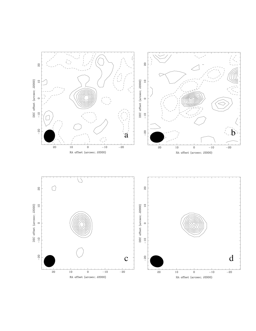
Figure 1: Images of both stars at 3 mm and 1 mm constructed from the combination of all available data. In each plot, contours are given at -20, -10, 10, 20, 30, 40, 50, 60, 70, 80, 90, 100% of the peak flux density. a) $\alpha$ Tau at 3 mm with a 13.97 mJy peak. b) $\alpha$ Tau at 1 mm with a 25.78 mJy peak. c) $\alpha$ Boo at 3 mm with a 20.09 mJy peak. The offset of the peak from the stellar position after allowance for proper motion is caused by the process of self-calibration. d) $\alpha$ Boo at 1 mm with a 83.5 mJy peak.

The final rows in Table 1 present the combined peak flux density information based on the totality of the available, good quality, stellar data for $\alpha$ Tau and $\alpha$ Boo. The corresponding combined images from which these final flux densities were determined appear as Figure 1.

4 Observations with LWS on ISO

Observations of $\alpha$ Tau with full wavelength coverage were made in three revolutions: 818 (TDT 81803302), 848 (TDT 84801701), and 861 (TDT 86101101). The observations of $\alpha$ Tau each consisted of 28 scans, 14 in each direction with a spectral oversampling of 4. Each observation had about 4630 s integration. LWS made two AOT observations of $\alpha$ Boo in revolutions 448 (TDT 44800303) and 608 (TDT 60800904), each with about 2300 s integration. These observations consisted of 12 scans, 6 in each direction, taken with an oversampling of 4.

Each LWS spectrum was processed with Offline Processing version 10 (OLP10) and all the data were reduced using the Infrared Spectral Analysis Package (ISAP). The reduction steps consisted of removing outliers and averaging over individual detectors at maximum resolution, clipping at 2.5$\sigma$. No attempt was made to scale the detectors to make the sub-spectra overlap in the reductions. We accomplished this outside ISAP using the splicing techniques described by Cohen et al. (1992b) for constructing absolutely calibrated spectra. Care was taken to use the same number of scans in each direction, so the effects due to transients in the data are minimal, and no transient correction was applied. The fundamental Uranus model for calibrating the LWS is a synthesis of globally averaged Voyager InfraRed Interferometer Spectrometer (IRIS) data up to 50 $\mu$m and James Clerk Maxwell Telescope data covering the 0.35–2 mm wavelength range (Griffin & Orton, 1993) with a radiative transfer model similar to the one described by Griffin & Orton (1993).

A formal off-source, full-grating, LWS integration is available only for $\alpha$ Boo (TDT 60801005), and two fixed-grating (sampling only ten wavelengths with no detector scans) observations exist (TDTs 21701113 and 27202302). However, it is vital to recognize that corrections for off-source emission in LWS are inappropriate for faint objects like normal stars in low-cirrus regions.

All observed LWS spectra have had the instrumental dark currents subtracted from them during the reductions. In our OLP10 reductions, we used the “fixed dark currents”, as determined in dedicated calibration observations. These LWS dark current measurements were essentially dark background measurements. The Fabry-Perot was placed in the beam and offset. Therefore, there was flux on the detectors, radiated by the 3.5-K blank, but this was negligible. The signals measured remained constant throughout the mission, and were subtracted from the measured photocurrents on-source. When the dark signal, measured from the blank, was compared with the signal measured on the dark patch of sky, no difference was found. Therefore, for dark sky, no additional “sky” subtraction is necessary. For regions with high cirrus, there is a sky signal in the LWS beam and, if a point source is being observed, an “off” position is needed to determine the local sky background. In dark regions, the sky flux predicted by COBE can form a substantial fraction of the LWS dark signal. However, this is deemed undetected, because no additional signal is detected over the signal from the blank.

Consequently, we must assess the measured sky background around the two K giants at those times when the LWS spectra were taken. If those backgrounds were below the fixed dark values, then there is no need for further subtraction of off-source LWS spectra. Indeed, that subtraction would produce meaningless stellar spectra by removing the dark currents twice. Both LWS and ISOPHOT, off-source, measure the sum of zodiacal (hereafter “zodi”), cirrus, and extragalactic emission, as did DIRBE. “IRSKY” shows that extragalactic and cirrus confusion noises are far below zodi, so the dominant background for the two K giants is zodi. We have used two methods to evaluate the FIR background near $\alpha$ Tau and $\alpha$ Boo: actual measurements in off-source pixels when these stars were observed in the FIR arrays of ISOPHOT; and, as a coarse check, DIRBE predictions for the LWS observations based on their solar elongation angles.

The computation of ISOPHOT background sky measurements near $\alpha$ Tau and $\alpha$ Boo is summarized in Tables 2 and  3. These present the relevant ISOPHOT observation by filter, nominal wavelength, TDT and measurement number, and the background brightness and its 1-$\sigma$ uncertainty. Our conversion from point source flux to surface brightness is different from the one given in the ISOPHOT handbook (Laureijs et al., 2003). The supporting analysis and justification are given by Schulz. When multiple data exist for a filter, inverse-variance weighted combinations of those data are also given. Conversion from MJy sr^-1 to F_λ (in W cm^-2 $\mu$m^-2) was accomplished using the published values for LWS detector beam solid angles, effective apertures, and bandwidths. Table 4 presents these backgrounds, and compares them with the fixed dark currents and DIRBE predictions (interpolated between 140 and 240 $\mu$m to assess the 160-$\mu$m values), matching each ISOPHOT band to the nearest LWS detector. The DIRBE predictions are generally in accord with ISOPHOT measurements. Clearly, the measured sky backgrounds around the two stars are all below the fixed dark currents, confirming that only low level cirrus appears in their vicinities (with the sole exception of $\alpha$ Boo in LW2, where ISOPHOT suggests 50% more sky brightness than the LW2 dark current). The DIRBE predictions are generally in accord with the ISOPHOT measurements. Subtraction of off-source LWS spectra would be inappropriate for these K giants.

Figures 2 and 3 illustrate our reduced, spliced LWS spectrum for each star, presenting the mean spectrum over all TDTs, with the $\pm 3\sigma$ bounds for $\alpha$ Tau (which has more LWS data, longer integrations, and higher SNR) and $\pm 2\sigma$ bounds for $\alpha$ Boo (with its noisier data sets). The sizeable triangular excursions in both spectra near 53 and 106 $\mu$m represent the difficulty, for NIR-bright normal stars, of mitigating the substantial leaks of 1.6-$\mu$m radiation to which LWS is prone. We have cleaned the observed spectra by 30-point boxcar smoothing of the data (equivalent to about a 2-$\mu$m interval). $\alpha$ Tau’s combined spectrum contained 1181 wavelength points; $\alpha$ Boo’s 706 points. Each figure incorporates the absolutely calibrated model continuum spectra that we have computed (see below) as the almost flat long-dashed lines that cross the figures, and the mean$\pm 1\sigma$ bounds on our older calibrated energy distributions (dash-triple-dotted lines) delivered in January 1996 for the calibration of ISOPHOT. To convert the model surface fluxes to predicted fluxes at the Earth, we have adopted the angular diameter, 20.88$\pm$0.10 mas, of Ridgway et al. (1982) (using lunar occultation) for $\alpha$ Tau and the angular diameter, 21.0$\pm$0.2 mas, of Quirrenbach et al. (1996) for $\alpha$ Boo (measured by optical intensity interferometry).

Our new, more detailed, calculations of stellar continuum spectra fall well within the uncertainties associated with the calibrated spectra originally delivered to ISO. We wish to quantify the degree of accord between measured and modeled spectra in the FIR for each star. The grating simultaneously illuminated the ten LWS detectors, and each detector was separately wavelength and flux calibrated. Therefore, LWS consists of ten spectrally independent detectors. The degree of oversampling of these stellar spectra was 4; consequently, adjacent points in Figures 2 and 3 are not independent. Therefore, to assess the consistency of observations and predictions, and to handle the dependence of adjacent LWS points in the fully-plotted spectra correctly, we include the data binned by detector as a series of bold crosses in Figures 2 and 3. Filled circles represent the inverse-variance weighted average of all the meaningful data in each LWS detector (e.g. after the rejection of data contaminated by $H$-band leaks). Error bars show the associated 1-$\sigma$ uncertainties. Asymmetric horizontal error bars represent the actual wavelength ranges usable for each detector and star. Filled circles are plotted at the average wavelength of each detector’s set of usable data for that star.

The binned detector data lie within 1$\sigma$ of the newly modeled energy distribution for $\alpha$ Tau, and within 1$\sigma$ for $\alpha$ Boo. There is good agreement between the underpinning Uranus calibration of LWS, the totally independently calibrated stellar spectra made from the empirical spectra by our older model extrapolations based on the available observations between 8 and 23 $\mu$m, and the newly calculated, absolutely calibrated, emergent stellar energy distributions. Averaging the results for the independent detectors for each star with inverse-variance weighting, we determine that, for $\alpha$ Tau, this mean scale factor is 1.000$\pm$0.011 (over nine detectors) while, for $\alpha$ Boo, this factor is 1.012$\pm$0.025 (over seven detectors). Therefore, empirical stellar and planetary calibrations used by ISO, and stellar modeling, are absolutely reconciled to 3.3% (3$\sigma$) for the better measured $\alpha$ Tau, and 7.5% (3$\sigma$) for the more poorly measured $\alpha$ Boo.

5 The Radiative Equilibrium Model Atmospheres

5.1 Atmospheric parameters and computation of the emergent spectrum

The spectrum calculations were carried out with the SOURCE model atmosphere program in essentially the same fashion as described in Carbon et al. (1982). Specifics pertinent to the current calculations are described in this section.

For $\alpha$ Tau, we adopted an effective temperature of 3920 K (Blackwell et al., 1991) and a log(g) of 1.5 (Smith & Lambert, 1990). For the isotopic abundances of C, N and O, we adopted log $\epsilon$(C) = 8.40, log $\epsilon$(N) = 8.20, log $\epsilon$(O) = 8.78, ¹²C/¹³C = 10, ¹⁶O/¹⁷O = 562, and ¹⁶O/¹⁸O = 475 (Harris & Lambert, 1984; Smith & Lambert, 1990). The remaining metal abundances were chosen to be solar, following the lead of Smith & Lambert (1985). The preceding abundances were derived using the MOOG spectrum synthesis code (Sneden, 1973) and model atmospheres (Johnson et al., 1980) constructed with the ATLAS (e.g., Kurucz (1993)) model atmosphere code and opacity sampling. Our choices of T_eff, log(g), and abundances are entirely consistent with current determinations of the parameters of $\alpha$ Tau. In particular, the values are well within the error bars of the values recently derived directly by Decin and her collaborators (Decin et al., 2000, 2003) from fits to stellar spectral energy distributions generated by using the MARCS (Gustafsson et al., 1975; Plez et al., 1992) model atmosphere code. Bertrand Plez (Plez, 1999) kindly computed an $\alpha$ Tau model atmosphere for us using the aforementioned parameters and the programs described in Plez et al. (1992). Thus, this model was computed with essentially the same model atmosphere program and opacities as employed by Decin.

For $\alpha$ Boo, we adopted a slightly revised version (Peterson (1995): hereafter PDK) of the Peterson et al. (1993) model atmosphere which has more depths than the original published model. This atmosphere has an effective temperature of 4300 K, log(g) of 1.5, [Fe/H] = -0.5, and other elemental abundances as determined by Peterson et al. (1993). The PDK model parameters derived by Peterson et al. (1993) were derived entirely from the observed stellar spectrum. As was the case for the Decin et al. investigation of $\alpha$ Tau, no assumptions were made regarding stellar temperature or gravity. We adopted all of the Peterson et al. (1993) values for our study. The parameters T_eff, gravity, microturbulent velocity, and [Fe/H] derived by Peterson et al. (1993) for $\alpha$ Boo are essentially identical to those derived later and independently by Decin et al. (2003), while the C, N, and O abundances agree within the error bounds.

The alert reader will observe that we have adopted model atmospheres for $\alpha$ Tau and $\alpha$ Boo that were derived using entirely different model atmosphere codes (ATLAS and MARCS). We shortly will describe results obtained by using these atmospheres as input to a third model atmosphere code, our SOURCE. We do not feel that significant improvement would result from insisting that only ATLAS or MARCS models be used in our study. All three codes have been vetted against the solar case and should give very comparable results in the G-K star domain. We cite as support for this stance the striking agreement between the results of Peterson et al. (1993) and Decin et al. (2003) for $\alpha$ Boo. This occurs despite Decin et al. (2003) having used a completely different model atmosphere program and blanketing representation (MARCS with opacity sampling) to compute their $\alpha$ Boo model than used by Peterson et al. (1993) (ATLAS with opacity distribution functions). The agreement is even more impressive when one considers that these two investigations derived their results from two entirely different spectral regions, 0.5–0.9 $\mu$m versus 2.38–12.0 $\mu$m. We regard this as evidence that different well-vetted model atmosphere codes and opacity representations now produce comparable model atmospheres and visible-infrared spectra for K-giants within the limited approximations of static, homogeneous atmospheres, LTE, and mixing-length-theory radiative/convective equilibrium. That does not mean that the resultant models are accurate, or even adequate, representations of a real star. Differences between observed and computed spectra are now much more likely to arise from the presence of physics (e.g., NLTE, non-radiative heat deposition, and inhomogeneous dynamical structure) not treated in the simple models we use here. We will discuss this point in more detail as we proceed.

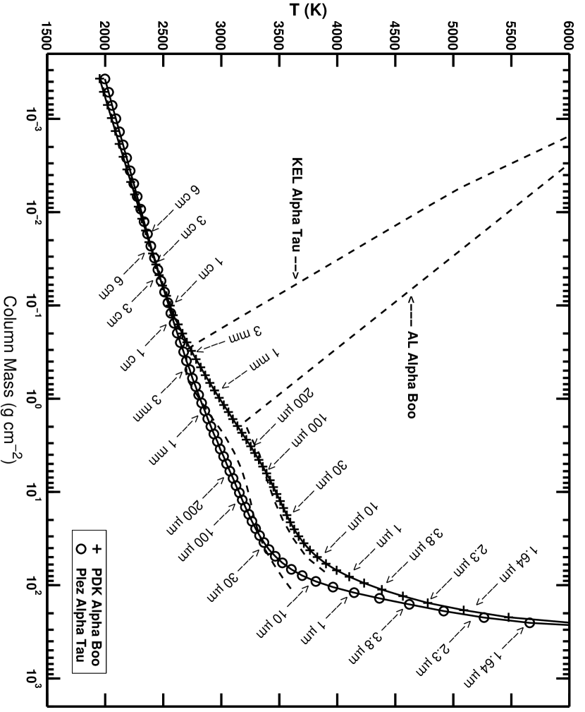
Figure 4: The adopted model atmosphere temperature structures for $\alpha$ Boo and $\alpha$ Tau. Arrows mark the depths at which optical depth unity is reached in the continuum at the indicated wavelengths. The upper set of arrows refers to the PDK model; the lower set, to the Plez model. For comparison, the AL and KEL chromosphere models are shown as dashed lines.

The column mass (g cm^-2) vs. temperature relations for both the Plez $\alpha$ Tau and PDK $\alpha$ Boo models were linearly extrapolated to shallower depths as required to obtain optical transparency at the longest wavelengths. For the Plez $\alpha$ Tau model, the extrapolated layers are shallower than 0.020 g cm^-2; for the PDK $\alpha$ Boo model, shallower than 0.010 g cm^-2. The resultant model atmospheres are shown in Figure 4.

It should be stressed that both of the above adopted model atmospheres have purely radiative equilibrium surface temperature structures. Specifically, they do not have chromospheric temperature rises, a point whose importance will become evident later. We have included in Figure 4, for comparison, the Kelch et al. (1978) (KEL) $\alpha$ Tau chromospheric model B and the Ayres & Linsky (1975) (AL) $\alpha$ Boo chromospheric model. These chromospheric models are semiempirical, derived from non-LTE analyses of Ca II and Mg II line fluxes. While these chromospheric models are now over 20 years old, they are very similar from the upper photosphere, through the temperature minimum region, and into the lower chromosphere to models of $\alpha$ Tau and $\alpha$ Boo used by Wiedemann et al. (1994), and the $\alpha$ Tau model derived by McMurry (1999).

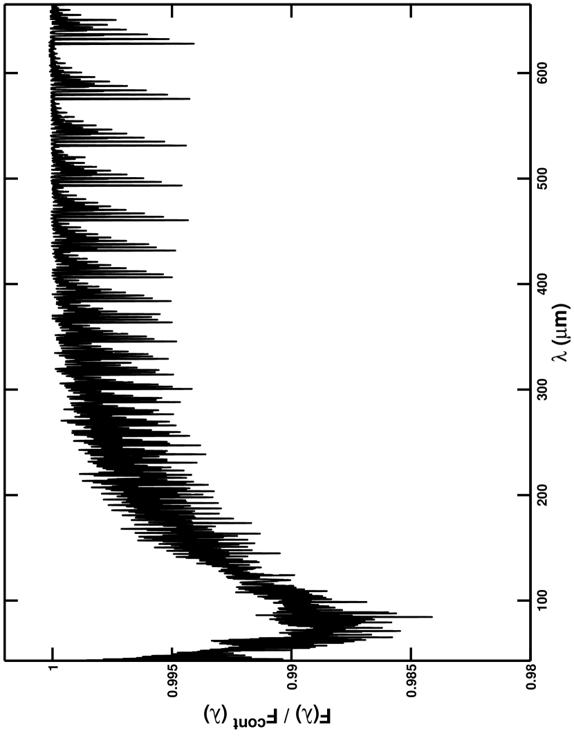
Figure 5: Continuum normalized flux predicted by the Plez $\alpha$ Tau model for the spectral range 43 $\mu$m to 665 $\mu$m. Note that the vertical scale is greatly magnified.

Using the Plez $\alpha$ Tau atmosphere and parameters detailed above, we have computed the synthetic spectrum for $\alpha$ Tau over the entire LWS range and beyond, 43 to 665 $\mu$m. The spectrum was computed using a full set of molecular line opacities which includes all the principal isotopomers of CO, SiO, OH, and ${\rm H_{2}O}$ and using a variable wavelength mesh which locally provides $\approx$2.5 points per Doppler width. To allow comparison with the LWS observations, we convolved the high-resolution result with a Gaussian instrumental profile function having a FWHM equal to 0.29 $\mu$m for $\lambda\leq$ 90.5 $\mu$m, and 0.60 $\mu$m, $\lambda>$ 90.5 $\mu$m (e.g., Gry et al. (2003)). The resulting spectrum, normalized to the continuum and on a greatly magnified ordinate scale, is shown in Figure 5. A detailed description of the displayed spectrum may be found in Carbon et al. (2005). We do note here that almost all the absorption beyond $\approx$ 50 $\mu$m is due to the isotopomers of SiO. At shorter wavelengths the principal contributor is OH with some H₂O and CO as well.

It is clear that, at the ISO LWS and the BIMA spectral resolutions, all differences between the pure continuum and the synthetic spectrum computed with the full set of molecular line opacities are less than 2%; beyond 130 $\mu$m, they are less than 1%. This is much less than the noise level in the observed $\alpha$ Tau spectra in this region. As a consequence, there is no significant advantage gained by using the full synthetic spectrum. For clarity in our presentation, we will use only the continuous spectrum in our comparisons with the $\alpha$ Tau observations. Since $\alpha$ Boo is both hotter and has lower metallicity, we shall use the continuum alone for comparisons there as well.

5.2 Depth of formation and brightness temperatures

For both the Plez $\alpha$ Tau and the PDK $\alpha$ Boo models, the dominant continuous opacity in the continuum-forming layers for wavelengths redward of the H^- opacity minimum at 1.64 $\mu$m arises from H^- free-free. This opacity increases in strength as $\lambda^{2}$. As a result, the emergent continuum flux is formed at progressively shallower layers in the stellar atmosphere as one proceeds to longer wavelengths. Figure 4 illustrates this point for the Plez $\alpha$ Tau and the PDK $\alpha$ Boo models. In this figure we have marked, for the radiative equilibrium models, the atmospheric depths for which the continuum optical depth, $\tau_{\lambda}^{c}$, reaches unity at the indicated wavelengths. That is, we have marked the column masses at which $\tau_{\lambda}^{c}$ = 1.0; roughly speaking, in the FIR, depths near this value and shallower make the greatest contribution to the emergent continuum flux at wavelength $\lambda$. Note, for example, that the continuum fluxes between 1 mm and 3 mm are sampling very different parts of the atmospheric temperature structure in both radiative equilibrium models than, say, the continuum fluxes at 2.3 $\mu$m. Indeed, the longest wavelengths are sampling, in the continuum, atmospheric levels reached only at the cores of lines in bluer portions of the spectrum. Only when one proceeds to the vacuum ultraviolet and its strong photoionization continua of metals is it possible to reach in the continuum the shallow atmospheric levels probed by the continuum at long wavelengths (e.g. Figure 1 of Vernazza et al. (1976)). Thus, the FIR continuum is an effective probe of the shallowest stellar layers which can supplement information derived from line cores and UV continua.

As noted above, there is very little difference between the full synthetic spectrum and the spectrum of the continuum. Figure 4 provides an important clue as to why spectral lines generally become less prominent at longer wavelengths. It is evident that, as one goes to shallower depths in the models, the slope of the temperature-column mass relation becomes smaller. The significance of this can be appreciated by considering an absorption line in the $\alpha$ Tau model with a characteristic, depth-independent, line core/continuum opacity ratio of 1000. If the absorption line occurs at a wavelength of 2.3 $\mu$m, the continuum will be formed at $\approx$5200 K and the line core will be formed at $\approx$3200 K. The same line at a wavelength of 200 $\mu$m will have the continuum formed at $\approx$3100 K and the line core at $\approx$2600 K, a much smaller temperature difference between line core and continuum than at 2.3 $\mu$m. Couple this with the decreasing temperature sensitivity of the Planck function as one goes to longer wavelengths and one has a recipe for progressively less prominent spectral features.

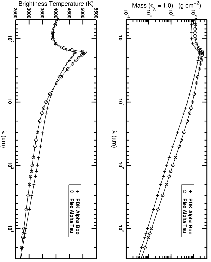
Figure 6: Upper panel: The column masses at which continuum optical depth unity is reached in the PDK $\alpha$ Boo and Plez $\alpha$ Tau radiative equilibrium models. Lower panel: The brightness temperatures predicted by the PDK $\alpha$ Boo and Plez $\alpha$ Tau radiative equilibrium models.

Figure 6 provides another window into the wavelength dependence of continuum formation. In the upper panel of Figure 6 we show the column masses for which $\tau_{\lambda}^{c}$ = 1.0 over the spectral range 0.5 $\mu$m to 200 $\mu$m. As noted above, there is a steady march to progressively shallower depths of continuum formation as one goes to longer wavelengths. Since the dominant H^- bound-free opacity peaks at roughly 0.825 $\mu$m, continuum fluxes at wavelengths between 0.825 $\mu$m and 1.64 $\mu$m probe the same atmospheric layers as continuum fluxes between 1.64 $\mu$m and 6.5 $\mu$m. Longward of 6.5 $\mu$m, the continuum flux probes atmospheric layers accessible only in line cores and in the metal bound-free continua of the vacuum ultraviolet.

In the lower panel of Figure 6 we show the continuum “brightness temperature” over the same spectral range for both models. The brightness temperature is defined as the temperature of a blackbody which gives the same flux as the model atmosphere at the indicated wavelength (a precise definition is given in Section 6.3). Three points are important. First, neither $\alpha$ Tau nor $\alpha$ Boo could have its continuum fluxes over any large spectral range matched by a blackbody of a single temperature. Second, the blackbody temperatures that do match the model fluxes at specific wavelengths are generally quite different than the effective temperatures of the models (or the stars) themselves. Third, comparing with Figure 4, one sees that the brightness temperature is systematically smaller than T($\tau_{\lambda}^{c}$ = 1.0), the temperature of the atmospheric layer at which optical depth unity is reached in the continuum at wavelength $\lambda$. (For an atmosphere with a linear source function at wavelength $\lambda$, the brightness temperature at $\lambda$ and T($\tau_{\lambda}^{c}$ = 2/3) would be identical. Unfortunately, in the particular cases of the PDK and Plez models, the FIR source functions are not linear in $\tau_{\lambda}^{c}$ but, rather, quadratic.) The differences between T($\tau_{\lambda}^{c}$ = 1.0) and brightness temperature vary systematically with wavelength. The differences are greatest at 1.64 $\mu$m and decrease to the red. Beyond 40 $\mu$m, the differences are always less than 100 K. (Had we chosen for illustration the more correct, but still approximate, T($\tau_{\lambda}^{c}$ = 2/3), the temperature differences would be smaller yet.) Thus, the brightness temperature is a good first guess at T($\tau_{\lambda}^{c}$ $\approx$ 1.0) at the longer wavelengths. Later, when we discuss differences between observed and predicted brightness temperatures, the reader may use this approximation and Figure 4 to roughly estimate the implied errors in the radiative equilibrium model temperature structures.

6 Discussion

6.1 Evidence for significant flux excesses at 1.4 mm and 2.8 mm

Table 5 shows the comparison between the observed fluxes and the predictions of the radiative equilibrium models. Only for the case of $\alpha$ Tau at 1.4 mm does there appear to be approximate agreement between the observed flux and the flux predicted from the radiative equilibrium model. The remainder of the observed fluxes are all significantly larger than the fluxes predicted by the models. The discrepancies are particularly striking in the case of $\alpha$ Boo.

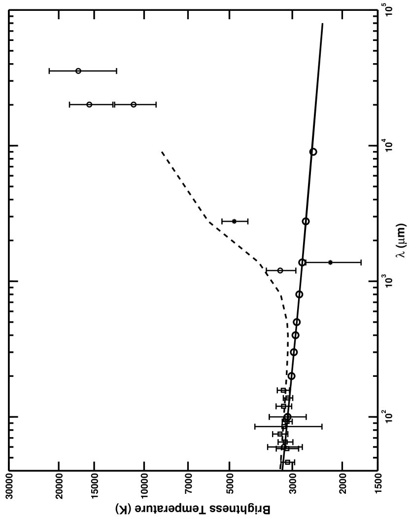
Figure 11: Brightness temperatures for $\alpha$ Tau including the predictions from the McMurry NLTE chromospheric model and from an independent computation using the LTE Plez model. Observations are marked exactly as in Figure 9 with the same error bars. We have magnified the vertical scale slightly to reduce the clutter of points. The brightness temperatures predicted by the McMurry NLTE chromospheric model are indicated as a dashed line. Brightness temperatures for the Plez model in LTE computed using MULTI are shown as open circles without error bars. Brightness temperatures predicted by SOURCE from the Plez model are shown by a solid line as before. Note that the brightness temperatures at cm wavelengths may be only upper limits. See the text for a discussion of the impact of wavelength dependent angular diameters.

We do not believe that the flux computation for the radiative equilibrium models could have errors sufficiently large to produce the marked differences between computed and observed millimeter fluxes. Our model atmosphere code has been carefully vetted and the dominant continuous opacities are themselves quite well determined (e.g., van der Bliek, Gustafsson, & Eriksson (1996)). (As an example of evidence for this, we refer the reader forward in the text to Figure 11. There we show the continuum for the Plez $\alpha$ Tau model computed with an entirely independent model code.) On the observational side, our derived errors for the observed 1.4-mm and 2.8-mm fluxes preclude dismissing the differences between observed and computed fluxes as simply due to measurement error. We believe other explanations must be considered.

Since the adopted angular diameters for these two stars appear to be extremely well determined, with standard deviations of $\approx$1% or less, they would not seem to be a significant source of error. Moreover, a major change in the angular diameters would compromise flux agreement for the $\lambda\leq$ 200 $\mu$m region. Nevertheless, it should be noted that the Quirrenbach et al. (1996) diameter is an arithmetic mean of values measured from 0.45 $\mu$m to 2.2 $\mu$m and the Ridgway et al. (1982) diameter is a error-weighted mean biased toward values obtained at 1.6 $\mu$m and 3.8 $\mu$m. At any particular monochromatic wavelength, an observed angular diameter represents the apparent diameter of the $\tau_{\lambda}$ $\approx$ 1.0 surface of the star. Since, as shown in Figures 4 and 6, there is a progressive march in depth of continuum formation to ever shallower atmospheric layers as one moves redward of 1.64 $\mu$m, the angular diameters themselves should increase with wavelength. If the angular diameters at 1.4 mm and 2.8 mm are substantially larger than those at the wavelengths of the Quirrenbach et al. (1996) and Ridgway et al. (1982) observations, our predicted fluxes in Table 5 could be seriously underestimated. We can roughly estimate the magnitude of this source of error, at least in the case of the radiative equilibrium models. In Table 6 we show the physical radii of $\alpha$ Tau and $\alpha$ Boo based on the indicated angular diameters and Hipparcos parallaxes (ESA, 1997). We also show the physical distances in the radiative equilibrium models between $\tau_{1.64\mu m}^{c}$ = 1.0 and $\tau_{2.8mm}^{c}$ = 1.0.

Given the tabulated numbers, it is clear that, for the PDK and Plez models, the atmospheric extent in the continuum at 2.8 mm is not sufficient to seriously affect our predicted fluxes. We find a similar result in the case of the only model chromosphere with a published height scale, McMurry’s chromospheric model for $\alpha$ Tau (McMurry, 1999). The McMurry atmosphere is plane-parallel and hydrostatic, constructed with log g = 1.25. Note that this gravity leads to a more distended atmosphere than does the higher gravity we adopted. The McMurry atmosphere has an extent of $\approx$2.6 $\times$ 10¹¹ cm between the layers where the 1.64 $\mu$m continuum is formed and the layer with T = 7120 K in the chromosphere. This extent is only 8% of the stellar radius and again seems too small to explain the discrepancy between computed and observed fluxes. Finally, as we will describe in Section 6.3, Drake & Linsky (1986) determined that $\alpha$ Boo has essentially the photospheric radius at 2 cm. Given the expected increase in angular diameter with wavelength, this would imply that $\alpha$ Boo would have the photospheric radius at $<$ 2 cm as well.

Based on the above arguments, we believe that the flux excesses observed at 1.4 mm and 2.8 mm, relative to the predictions of the purely radiative models, are real and significant. Furthermore, as we shall show, there is good evidence that these excesses are signatures of the chromospheric temperature rise in the two red giants.

6.2 Other observations of the sub-mm through cm region

Figures 7 and 8 present our millimeter flux densities (filled circles) and the color-corrected IRAS measurements of each star at 12, 25, 60, and 100 $\mu$m (crosses). Each figure includes the Plez $\alpha$ Tau or PDK $\alpha$ Boo spectrum, as appropriate, from 10 $\mu$m to 3 mm.

There are additional high-frequency radio continuum observations of these two K giants in the literature. Altenhoff et al. (1986) made single-dish 86-GHz measurements of $\alpha$ Boo (21.4$\pm$7.5 mJy) with the IRAM 30-m telescope, while Altenhoff et al. (1994) likewise detected both $\alpha$ Tau and $\alpha$ Boo at 250 GHz, obtaining 51$\pm$6 and 78$\pm$8 mJy, respectively. There are also VLA centimeter measurements on both stars at 4.9, 8.4, and 14.9 GHz by Drake & Linsky (1986), and unpublished data by Drake, Linsky, & Judge from the compilation of radio data by Wendker (1995). These long wavelength measurements all have substantial uncertainties, in part due to the faintness of the stars, in part to the potential for confusion with extragalactic background objects. Nonetheless, in combination with our own radio data (Figures 7, 8) one sees that these high-frequency data (open diamonds) are in good agreement with our aperture synthesis measurements (filled circles).

6.3 Brightness temperatures for all the observed fluxes

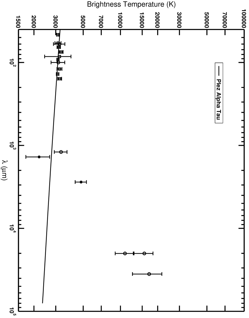
Figure 9: Brightness temperatures corresponding to the observed and computed fluxes for $\alpha$ Tau which have been discussed in this paper. LWS observations are represented by open squares, our mm measurements by asterisks, all other observations by open circles. Error bars represent 1-$\sigma$ deviations in the fluxes only; errors for 2-cm and 3.6-cm points are our own estimates (see text). Brightness temperatures predicted by the Plez model are shown by a solid line. Note that the brightness temperatures at cm wavelengths may be only upper limits. See the text for a discussion of the impact of wavelength dependent angular diameters.

It is difficult to fully appreciate the significance of the excess fluxes from the logarithmic scales of Figures 7 and 8. An insightful alternative view may be obtained by combining the mm and cm fluxes from other observers with our data and looking at the whole dataset as brightness temperatures over a broad spectral range. In Figures 9 and 10 we show the brightness temperatures corresponding to all the observed flux data between 43 $\mu$m and 6 cm used in our previous figures. For comparison we have also plotted the predictions of the radiative equilibrium models. In deriving brightness temperatures from the observed fluxes, we used the angular diameters of Table 6 in the following relation:

$$T_{B}(\lambda)=\frac{14387.75\>/\>\lambda}{\ln(\>1\;+\;\frac{733.4090\>\alpha^{2}}{S_{Jy}(\lambda)\>\lambda^{3}})}$$

where $S_{Jy}(\lambda)$ is the observed flux in Jy, $\alpha$ is the angular diameter in mas, $\lambda$ is the wavelength in microns, and $T_{B}(\lambda)$ is in Kelvins. The error bars in Figures 9 and 10 correspond only to the uncertainties in the observed fluxes. In the case of the $\alpha$ Tau data at 2 cm and 3.6 cm, no error values were reported by Wendker (1995) and we used our own rough estimates of the plausible errors. Before proceeding, a caveat needs to be noted regarding the longer wavelength points especially. The observed fluxes presumably come from progressively shallower stellar layers as $\lambda$ increases. All of the brightness temperatures in Figures 9 and 10 have been deduced assuming the photospheric angular diameters of Table 6. Atmospheric extension may play a role in the chromospheric layers of $\alpha$ Tau and $\alpha$ Boo. Carpenter et al. (1985) estimated the extension of the chromospheres of these stars. They argued that the C II UV 0.01 lines which they studied were formed in chromospheric layers with temperatures of $\approx$10000 K in $\alpha$ Tau and $\approx$8000 K in $\alpha$ Boo. They deduced that these chromospheric layers had radii of $\approx$2.0 R_∗ and $\approx$1.4 R_∗, respectively, where R_∗ is the stellar photospheric radius. Although these estimates are, in the authors’ words, “relatively crude”, they do suggest that atmospheric extension may play a role at least in the hotter layers of the chromosphere. Different evidence of extension was found by Drake & Linsky (1986) in their study of 2 cm and 6 cm fluxes. They treated all the radio emission as coming from an optically thick ionized wind for which a “half-power radius” could be deduced. In the case of $\alpha$ Boo they found the 2 cm half-power radius was $\approx$R_∗; at 6 cm, the half-power radius had grown to $\approx$1.7 R_∗. Taking the long wavelength approximation to the brightness temperature expression above, we see that, for a given observed flux, $T_{B}(\lambda)\propto~{}1/\alpha^{2}$, where $\alpha$ is the angular diameter. Since the shallowest layers may have angular diameters significantly larger than those of the photosphere, the corresponding brightness temperatures in Figures 9 and 10 should be regarded as upper limits.

6.4 Evidence for contributions from a stellar chromosphere

We now describe why we believe that the flux excesses at the longer wavelengths arise from the presence of stellar chromospheres in $\alpha$ Boo and $\alpha$ Tau.

6.4.1 Circumstantial Evidence

Circumstantial evidence suggests the possibility that stellar chromospheres could explain the flux excesses. This evidence comes by examining the depths at which $\tau_{\lambda}^{c}$ = 1.0. In the case of $\alpha$ Boo, as shown in Figure 4, the AL chromospheric model departs from the purely radiative equilibrium model at a column mass of $\approx$ 0.75 g cm^-2 (Ayres & Linsky, 1975). This is just in the column mass range of the PDK radiatve equilibrium model where optical depth unity is reached between 200 $\mu$m and 1 mm. Given this, it is not surprising that the PDK model might significantly underpredict the flux at both 1.4 mm and 2.8 mm in $\alpha$ Boo. We believe that the progressively larger differences between the predictions of the PDK model and the observations beyond 120 $\mu$m are due to the contributions of $\alpha$ Boo’s chromosphere.

The circumstantial evidence in the case of $\alpha$ Tau is not so clear. As shown in Figure 4, the KEL $\alpha$ Tau chromospheric model begins its temperature rise at a column mass of $\approx~{}$0.3 g cm^-2 (Kelch et al., 1978). This is slightly shallower in the Plez $\alpha$ Tau model than where $\tau_{3~{}mm}^{c}$ = 1.0 occurs. Nevertheless, the 2.8 mm observed brightness temperature is distinctly higher than that predicted by the Plez model in Figure 9. In fact, with the exception of our 1.4 mm point, the general run of observed points beyond 200 $\mu$m suggests that some enhanced (chromospheric?) emission may be present at 1 mm or even shorter wavelengths. Whether this is true or not will take additional observations in this spectral region with better SNR.

6.4.2 Evidence from NLTE modeling

While NLTE chromospheric modeling is well beyond the intent of this investigation, one of us (ADM) has computed the infrared fluxes predicted by his chromospheric model of $\alpha$ Tau . Details of the model and the NLTE computation may be found in McMurry (1999). This model is essentially identical to the KEL model from the photosphere through the lower and middle chromosphere, differing from the KEL model only at column masses shallower than 10^-3 g cm^-2 (see Fig. 5, McMurry (1999)). The NLTE radiative transfer computation was carried out with the independent code MULTI. We show in Figure 11 the results of this NLTE computation with a chromospheric model compared with the observations, and with the predictions of the Plez model.

It is immediately apparent that, again with the exception of our 1.4 mm point, the observed data beyond 200 $\mu$m is better fit by the NLTE chromosphere model than the LTE Plez radiative equilibrium model. We believe this is good evidence that the stellar chromosphere of $\alpha$ Tau has a significant impact on the observed fluxes beyond 200 $\mu$m. Indeed, it should be noted that the fit is even improved between 100 $\mu$m and 200 $\mu$m.

6.5 The transition from photosphere to chromosphere

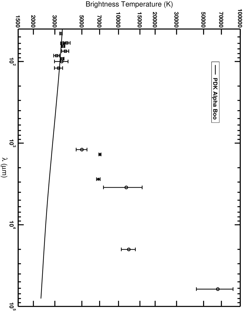
Figure 10: Brightness temperatures corresponding to the observed and computed fluxes for $\alpha$ Boo which have been discussed in this paper. LWS observations are represented by open squares, our mm measurements by asterisks, all other observations by open circles. Error bars represent 1-$\sigma$ deviations in the fluxes only. Brightness temperatures predicted by the PDK model are shown by a solid line. Note that the brightness temperatures at cm wavelengths may be only upper limits. See the text for a discussion of the impact of wavelength dependent angular diameters.

For $\alpha$ Boo (Figure 10) it appears that the transition from purely radiative occurs beyond 120 $\mu$m, and certainly well before 1.4 mm. In our opinion this makes any purely radiative model for $\alpha$ Boo a poor choice for calibration in the sub-mm spectral region. This appears to be the case for $\alpha$ Tau as well, especially considering the predictions of the McMurry chromospheric model (Figure 11). Given the evidence described above, we do not believe that it is prudent to use cool star radiative models for calibration purposes at the longer wavelengths unless alternatively calibrated observations already confirm the validity of the purely radiative models. One must be certain that the flux predicted by the purely radiative model at the long wavelength end of the region being calibrated by the theoretical stellar spectrum does indeed correspond to the actual star. In other words, we believe that when one is approaching the spectral regions where a chromospheric contribution can be significant, one can safely use purely radiative cool star models only as an interpolation tool for calibrations, not as an extrapolation tool.

We would like to emphasize the importance of the spectral region from $\approx$30 $\mu$m to several millimeters to furthering an understanding of cool stellar atmospheres. Fluxes from this spectral region reflect the mean time- and spatial-averaged emission from the upper photosphere and chromosphere for stars like those we consider here (see Figure 4). Accurate fluxes measured through this spectral region should allow one to test directly model atmosphere structures, even complex ones that include NLTE and dynamics, over the very interesting depth range in which non-radiative processes like shocks begin to alter the structure. By selectively sampling progressively longer wavelengths, one can follow the important transition from photosphere to chromosphere, locating the depth at which purely radiative models like the PDK and Plez models begin to fail.

6.6 Stellar absolute calibrators for ISOPHOT

Our original, theoretically extrapolated, continuum spectra for the two K giants, supplied to ISOPHOT as absolutely calibrated energy distributions, are in extremely good agreement with our new calibrated synthetic spectra (Figures 2, 3), well within the $\pm$6% uncertainties assigned to the original calibrators (Cohen et al., 1996b). The LWS spectra, reduced with respect to Uranus as calibrator, are consistent with the new (and old) synthetic spectra, thereby uniting FIR planetary and stellar calibrations at the few percent level (Figures 2, 3).

There are independent data on $\alpha$ Boo, derived from the validation of ISOPHOT’s final pipeline (OLP10) (Richards, 2003), that show it conforms to our 1996 model spectrum. In addition, Schulz (2003) has described the performance through the ISO mission of a significant number of ISOPHOT calibrators. By removing the contributions made by any particular source to the calibration process, and calibrating that source with respect to all other calibrators, one can assess the ratio of observed to modeled irradiance. Using the database described by Schulz (2003), we have been able to extend the range over which our new model of $\alpha$ Boo can be tested, and to validate $\alpha$ Tau independently of our LWS data. For $\alpha$ Boo, we have determined the observed to modeled irradiance ratios for the ISOPHOT C100, C120, C135, C160, C180, and C200 filters (“C” denotes the FIR camera within the ISOPHOT instrument, and each filter is designated by its reference wavelength in $\mu$m). Expressing these observed irradiance ratios with respect to our new modeled spectrum for $\alpha$ Boo we find: C100, 1.02$\pm$0.02; C120, 1.14$\pm$0.08; C135, 1.01$\pm$0.02; C160, 1.06$\pm$0.02; C180, 1.00$\pm$0.03; C200, 1.00$\pm$0.26. For $\alpha$ Tau, measurements are available solely in the C160 filter and yield a ratio of 0.96$\pm$0.05, with respect to our new model. We conclude that the separate absolute calibrations of LWS and ISOPHOT are in accord within the uncertainty of the observations, despite their different dependences on planets, asteroids, and stars. This should not be interpreted to mean that more accurate observations might not reveal discrepancies between FIR observations and the predictions of static, LTE model atmospheres computed in simple radiative/convective equilibrium.

7 Conclusions

Our primary objective was to investigate whether purely radiative models for two normal K giants could reproduce the observed FIR and microwave fluxes. We have found that for both $\alpha$ Tau and $\alpha$ Boo the radiative equilibrium temperature structures of the upper photospheres produce fluxes in agreement with the observations, but only up to a certain point. For $\alpha$ Boo and $\alpha$ Tau the agreement extends to at least 125 $\mu$m, corresponding to a column mass of $\approx$5 gm cm^-2 in the PDK atmosphere and $\approx$10 gm cm^-2 in the Plez atmosphere. Both K giants clearly show definite chromospheric emission at 2.8 mm. In $\alpha$ Boo this is evident by 1.4 mm. Only additional observations can pinpoint precisely where between 125 $\mu$m and 2.8 mm the chromospheric contribution becomes significant. For this reason, we cannot rely on purely radiative model atmospheres to form a basis for stellar calibration in the sub-mm region. Purely radiative models of the continuum might be used to provide calibrations between those shorter FIR wavelengths where the validity of the model fluxes already has been independently verified by observations.

Finally, our results indicate that accurate FIR, sub-mm, and mm observations can provide valuable new information for researchers modeling stellar chromospheres of cool stars.

Figure 2: LWS spectrum of $\alpha$ Tau showing the mean observed spectrum (solid line) after boxcar smoothing, and the mean$\pm 3\sigma$ bounds (short-dashed lines), compared with the Plez model continuum spectrum (long-dashed lines) and with the mean$\pm 1\sigma$ bounds on the old SED provided to ISOPHOT in 1996 (dash-triple-dotted lines). Each detector result is shown as a heavy cross, where horizontal bars represent the actual wavelength extent of the useful data, and vertical bars show the 1-$\sigma$ errors on the plotted weighted-mean points.

Figure 3: LWS spectrum of $\alpha$ Boo showing the mean observed spectrum (solid line) after boxcar smoothing, and the mean$\pm 2\sigma$ bounds (short-dashed lines), compared with the PDK model continuum spectrum (long-dashed lines) and with the mean$\pm 1\sigma$ bounds on the old SED provided to ISOPHOT in 1996 (dash-triple-dotted lines). Heavy crosses as for Fig. 2.

Figure 7: FIR to cm spectrum of $\alpha$ Tau. Color-corrected IRAS points (crosses) are plotted together with our mm observations (filled circles), the LWS spectrum (solid), and our computed continuum spectrum (dashed line). Also shown are mm and cm data from the literature (open diamonds).

Figure 8: FIR to mm spectrum of $\alpha$ Boo as for Figure 7.

Table 1: Journal of observations

Star	Date	Array	Frequency	Time	Phase	Secondary	Primary	Traceable	Peak Fν
			GHz	on star	Ref.	Flux Ref.	Flux Ref.	to Primary	mJy
$\alpha$ Tau	14Nov97	C	106.6845	4.32 hr	0449+113	3C111	Mars,	$\cdots$	17.14$\pm$2.19
$\cdots$	$\cdots$	$\cdots$	$\cdots$	$\cdots$	$\cdots$	$\cdots$	Uranus, Neptune	$\cdots$	$\cdots$
$\alpha$ Boo	15Nov97	C	106.6845	4.22 hr	1415+133	3C111	Mars,	$\cdots$	20.27$\pm$2.95
$\cdots$	$\cdots$	$\cdots$	$\cdots$	$\cdots$	1357+193	$\cdots$	Uranus, Neptune	$\cdots$	$\cdots$
$\alpha$ Boo	15Nov97	C	110.1282	4.22hr	1415+133	3C111	Mars,	$\cdots$	18.47$\pm$2.73
$\cdots$	$\cdots$	$\cdots$	$\cdots$	$\cdots$	1357+193	$\cdots$	Uranus, Neptune	$\cdots$	$\cdots$
$\alpha$ Boo	15Nov97	C	Both	$\cdots$	$\cdots$	$\cdots$	$\cdots$	$\cdots$	19.73$\pm$2.16
$\alpha$ Tau	06Jun98	C	106.6845	2.99hr	0449+113	3C111	Mars	$\cdots$	13.10$\pm$3.40
$\alpha$ Boo	11Mar99	B	106.6845	$\cdots$	1357+193	1415+133	$\cdots$	Mars	24.57$\pm$1.20
$\alpha$ Boo	11Mar99	B	110.1282	4.37 hr	1357+193	1415+133	$\cdots$	Mars	19.68$\pm$1.23
$\alpha$ Boo	11Mar99	B	Both	$\cdots$	$\cdots$	$\cdots$	$\cdots$	$\cdots$	22.03$\pm$0.97
$\alpha$ Boo	12Mar99	B	106.6845	3.13 hr	1357+193	1415+133	MWC 349, Mars	Mars	21.02$\pm$1.74
$\alpha$ Boo	12Mar99	B	110.1282	$\cdots$	1357+193	1415+133	MWC 349, Mars	Mars	18.90$\pm$1.20
$\alpha$ Boo	12Mar99	B	Both	$\cdots$	$\cdots$	$\cdots$	$\cdots$	$\cdots$	19.92$\pm$1.02
$\alpha$ Tau	05Sep99	D	216.0982	1.85 hr	0530+135	0530+135	$\cdots$	MWC 349/Mars	24.23$\pm$6.87
$\alpha$ Tau	05Sep99	D	219.5418	$\cdots$	0530+135	0530+135	$\cdots$	MWC 349/Mars	27.34$\pm$8.12
$\alpha$ Tau	05Sep99	D	Both	$\cdots$	$\cdots$	$\cdots$	$\cdots$	$\cdots$	25.78$\pm$5.64
$\alpha$ Boo	01Jun00	D	216.0982	2.91 hr	3C273	3C273	MWC 349	Mars	81.55$\pm$2.35
$\alpha$ Boo	01Jun00	D	219.5418	2.91 hr	3C273	3C273	MWC 349	Mars	85.45$\pm$2.44
$\alpha$ Boo	01Jun00	D	Both	$\cdots$	$\cdots$	$\cdots$	$\cdots$	$\cdots$	83.50$\pm$1.71
$\alpha$ Tau	09Dec00	C	106.6845	3.19 hr	3C111	3C111	W3OH, Mars,	$\cdots$	12.55$\pm$2.16
$\cdots$	$\cdots$	$\cdots$	$\cdots$	$\cdots$	$\cdots$	$\cdots$	Uranus	$\cdots$	$\cdots$
$\alpha$ Tau	09Dec00	C	110.1282	3.19 hr	3C111	3C111	W3OH, Mars,	$\cdots$	12.77$\pm$2.95
$\cdots$	$\cdots$	$\cdots$	$\cdots$	$\cdots$	$\cdots$	$\cdots$	Uranus	$\cdots$	$\cdots$
$\alpha$ Tau	09Dec00	C	Both	$\cdots$	$\cdots$	$\cdots$	$\cdots$	$\cdots$	12.40$\pm$1.91
$\alpha$ Tau	All	All	108.40	$\cdots$	$\cdots$	$\cdots$	$\cdots$	$\cdots$	13.97$\pm$1.46
$\alpha$ Tau	All	All	217.82	$\cdots$	$\cdots$	$\cdots$	$\cdots$	$\cdots$	25.78$\pm$5.64
$\alpha$ Boo	All	All	108.40	$\cdots$	$\cdots$	$\cdots$	$\cdots$	$\cdots$	20.09$\pm$0.69
$\alpha$ Boo	All	All	217.82	$\cdots$	$\cdots$	$\cdots$	$\cdots$	$\cdots$	83.50$\pm$1.71

Table 2: ISOPHOT measurements of sky background near $\alpha$ Tau

Filter	$\lambda$	TDT	Meas.#	Background$\pm$Unc.
	($\mu$m)			(MJy sr-1)
C1-100	100	86401601	2	42.32$\pm$3.57
C1-100	100	86401602	2	44.53$\pm$2.68
C2-160	170	86002102	1	43.06$\pm$4.39
C1-60	60	84300501	5	34.54$\pm$4.68
C1-100	100	84300501	2	36.69$\pm$4.14
C1-60	60	84300501	5	40.89$\pm$5.53
C1-60	60	combined	$\cdots$	37.19$\pm$3.57
C1-100	100	combined	$\cdots$	42.24$\pm$1.90

Table 3: ISOPHOT measurements of sky background near $\alpha$ Boo

Filter	$\lambda$	TDT	Meas.#	Background$\pm$Unc.
	($\mu$m)			(MJy sr-1)
C1-50	50	27501511	1	18.16$\pm$1.42
C1-90	90	27502117	1	14.62$\pm$0.87
C1-105	105	27500602	1	12.54$\pm$0.54
C1-105	105	27500602	1	11.56$\pm$0.94
C2-120	120	27503008	1	9.10$\pm$1.16
C2-135	135	27503311	1	8.73$\pm$1.12
C2-160	170	27503614	1	9.23$\pm$0.96
C2-160	170	27503614	1	8.34$\pm$0.27
C2-200	200	27502402	1	6.61$\pm$0.39
C1-105	105	combined	$\cdots$	12.30$\pm$0.47
C2-160	170	combined	$\cdots$	8.41$\pm$0.26

Table 4: Comparison of ISOPHOT sky backgrounds and fixed dark currents in W cm^-2 $\mu$m^-1

Star	ISOPHOT	Nearest	Fixed	ISOPHOT	DIRBE
	Band	LWS det.	Dark	Sky	zodi
$\alpha$ Tau	C1-60	SW2	4.2E-18	4.5E-19	3.8E-19
$\alpha$ Tau	C1-100	LW1	8.0E-19	1.3E-19	1.1E-19
$\alpha$ Tau	C2-160	LW4	9.1E-20	4.5E-20	5.9E-20
$\alpha$ Boo	C1-50	SW2	4.2E-18	2.0E-19	$>$1.3E-19
$\alpha$ Boo	C1-90	SW5	3.2E-18	8.7E-20	$\cdots$
$\alpha$ Boo	C1-105	LW1	8.0E-19	5.2E-20	2.7E-20
$\alpha$ Boo	C2-120	LW2	7.7E-21	1.2E-20	1.2E-20
$\alpha$ Boo	C2-135	LW3	2.0E-20	1.7E-20	7.0E-21
$\alpha$ Boo	C2-160	LW4	9.1E-20	1.5E-20	1.8E-20
$\alpha$ Boo	C2-200	LW5	4.4E-19	8.6E-21	$\cdots$

Table 5: Radiative models: fluxes and brightness temperatures

Frequency	Quantity	$\alpha$ Boo	$\alpha$ Tau
217.820 GHz (1.376 mm)	Observed Flux (mJy)	83.50$\pm$1.71	25.78$\pm$5.64
$\cdots$	Predicted Flux (mJy)	33.43	32.38
$\cdots$	$\mid$Predicted–Observed Flux$\mid$/$\sigma$(observed)	29.3	1.17
$\cdots$	Observed Brightness Temperature (K)	7040$\pm$140	2200$\pm$480
$\cdots$	Predicted Brightness Temperature (K)	2820	2760
108.406 GHz (2.765 mm)	Observed Flux (mJy)	20.09$\pm$0.69	13.97$\pm$1.46
$\cdots$	Predicted Flux (mJy)	7.94	7.80
$\cdots$	$\mid$Predicted–Observed flux$\mid$/$\sigma$(observed)	17.6	4.23
$\cdots$	Observed Brightness Temperature (K)	6840$\pm$230	4810$\pm$500
$\cdots$	Predicted Brightness Temperature (K)	2700	2690

Table 6: Radiative Models: atmospheric extents

Quantity	$\alpha$ Boo	$\alpha$ Tau
Adopted angular diameter (mas)	21.0$\pm$0.2	20.88$\pm$0.10
Adopted parallax (mas)	88.85$\pm$0.74	50.09$\pm$0.95
Deduced stellar radius (cm)	1.77 x 1012	3.12 x 1012
1.64 $\mu$m - 2.8 mm atmospheric thickness (cm)	4.38 x 1010	4.22 x 1010
Percentage of stellar radius	2.5%	1.4%

References

- Altenhoff et al. (1986) Altenhoff, W. J., Huchtmeier, W. K., Schmidt, J., Schraml, J. B., & Stumpff, P. 1986, A&A, 164, 227
- Altenhoff et al. (1994) Altenhoff, W. J., Thum, C., & Wendker, H. J. 1994, A&A, 281, 161
- Ayres et al. (1997) Ayres, T.R., Brown, A., Harper, G.M., Bennett, P.D., Linsky, J.L., Carpenter, K.G., & Robinson, R.D. 1997, ApJ, 491, 876
- Ayres & Linsky (1975) Ayres, T.R. & Linsky, J.L. 1975, ApJ, 200, 660
- Blackwell et al. (1991) Blackwell, D.E., Lynas-Gray, A.E., & Petford, A.D. 1991, A&A, 245, 567
- van der Bliek, Gustafsson, & Eriksson (1996) van der Bliek, N.S., Gustafsson, B. & Eriksson, K. 1996, A&A, 309, 849
- Carbon et al. (1982) Carbon, D.F., Langer, G.E., Butler, D., Kraft, R.P., Trefzger, Ch.F., Suntzeff, N.B., Kemper, E., & Romanishin, W. 1982, ApJS, 49, 207
- Carbon et al. (2005) Carbon, D.F., Idehara, H., & Goorvitch, D. 2005, AJ, in preparation
- Carpenter et al. (1985) Carpenter, K.G., Brown, A., & Stencel, R.E. 1985, ApJ, 289, 676
- Clegg et al. (1996) Clegg, P. E. et al. 1996, A&A, 315, L38
- Cohen (1998) Cohen, M. 1998, AJ, 115, 2092
- Cohen & Davies (1995) Cohen, M. & Davies, J. K. 1995, MNRAS, 276, 715
- Cohen et al. (2003a) Cohen, M., Megeath, T.G., Hammersley, P.L., Martin-Luis, F., & Stauffer, J. 2003, AJ, 125, 2645
- Cohen et al. (2003b) Cohen, M., Wheaton, W.A., & Megeath, T.G. 2003, AJ, 126, 1090
- Cohen et al. (1992a) Cohen, M., Walker, R.G., Barlow, M.J., & Deacon, J.R., 1992a, AJ, 104, 1650
- Cohen et al. (1999) Cohen, M., Walker, R.G., Carter, B., Hammersley, P., Kidger, M., & Noguchi, K., 1999, AJ, 117, 1864
- Cohen et al. (2001) Cohen, M., Walker, R.G., Jayaraman, S., Barker, E., & Price, S.D. 2001, AJ, 121, 1180
- Cohen et al. (1992b) Cohen, M., Walker, R. G., & Witteborn, F. C. 1992b, AJ, 104, 2030
- Cohen et al. (1996a) Cohen, M., Witteborn, Bregman, J. D., Wooden, D.H., Salama, A., and Metcalfe, L. 1996, AJ, 112, 241
- Cohen et al. (1992c) Cohen, M., Witteborn, F. C., Carbon, D. F., Augason, G. C., Wooden, D.H., Bregman, J. D., & Goorvitch, D. 1992c, AJ, 104, 2045
- Cohen et al. (1996b) Cohen, M., Witteborn, F. C., Carbon, D. F., Davies, J. K., Bregman, J. D., & Wooden, D. H. 1996b, AJ, 112, 2274
- Cohen et al. (1995) Cohen, M., Witteborn, F.C., Walker, R.G., Bregman, J.D., & Wooden, D.H. 1995, AJ, 110, 275
- Decin et al. (2000) Decin, L., Waelkens, C., Eriksson, K., Gustafsson, B., Plez, B., Sauval, A.J., Van Assche, W., & Vandenbussche, B. 2000, A&A, 364, 137
- Decin et al. (2003) Decin, L., Vandenbussche, B., Waelkens, C., Decin, G., Eriksson, K., Gustafsson, B., Plez, B., & Sauval, A.J. 2003, A&A, 400, 709
- Drake & Linsky (1986) Drake, S. A. & Linsky, J. L. 1986, AJ, 91, 602
- Dreher & Welch (1983) Dreher, J.W. & Welch, W.J. 1983, AJ, 88, 1014
- ESA (1997) ESA 1997, The Hipparcos and Tycho Catalogues, ESA SP-1200, or http://astro.estec.esa.nl/Hipparcos/catalog.html
- Gibson et al. (2005) Gibson, J., Welch, W. J., & de Pater, I. 2005, Icarus, in press
- Griffin & Orton (1993) Griffin, M. & Orton, G. 1993, Icarus, 105,537
- Gry et al. (2003) Gry, C. et al. 2000, in “The ISO Handbook, Vol. III: LWS - The Long-Wavelength Spectrometer” (ESA SP-1262)
- Gustafsson et al. (1975) Gustafsson, B., Bell, R. A. Eriksson, K., & Nordlund, A. 1975, A&A, 42, 407
- Harris & Lambert (1984) Harris, M.J. & Lambert, D.L. 1984, ApJ, 285, 674
- Johnson et al. (1980) Johnson, H. R. Bernat, A. P. Krupp, B. M. 1980, ApJS, 42, 501
- Laureijs et al. (2003) Laureijs, R. J., Klaas, U., Richards, P. J., Schulz, B., & Abraham, P. 2003, “The ISO Handbook Vol. IV: PHT - The Imaging Photo-Polarimeter” (ESA SP-1262)
- Kelch et al. (1978) Kelch, W.L., Linsky, J.L., Basri, G.S., Chiu, H.-Y., Chang, S.-H., Maran, S.P., & Furenlid, I. 1978, ApJ, 220, 962
- Kessler et al. (1996) Kessler, M.F. et al. 1996, A&A, 315, L27
- Kurucz (1993) Kurucz, R. 1993, ATLAS9 Stellar Atmosphere Programs 2 km/s grid. Kurucz CD-ROM No. 13. Cambridge, Mass.: Smithsonian Astrophysical Observatory, 1993
- Lemke et al. (1996) Lemke, D. et al. 1996, A&A, 315, L64
- Lim et al. (1997) Lim, T., Swinyard, B.M., Liu, X.-W., Burgdorf, M., Gry, C., Pezzuto, S., & Tommasi, E. 1997, “First ISO Workshop on Analytical Spectroscopy”, eds. A.M. Heras, K. Leech, N.R. Trams & M. Perry, ESA SP-419, pg. 281
- Linsky & Haisch (1979) Linsky, J.L., & Haisch, B.M. 1979, ApJ, 229, L27
- McMurry (1999) McMurry, A.D. 1999, MNRAS, 302,37
- Mill et al. (1994) Mill, J. et al. 1994, AIAA, 31, 900
- Mitchell et al. (1996) Mitchell, K. J. et al. 1996, in “Unveiling the Cosmic Background”, ed. E. Dwek (AIP, CP 348), p.301
- Muller & Lagerros (1998) Muller, T.G. & Lagerros, J.S.V. 1998, A&A, 338, 340
- Murakami et al. (1997) Murakami, H. et al. 1996, PAS Japan, 48, L41
- Orton et al. (2000) Orton, G., Burgdorf, M., Davis, G., Sidher, S., Griffin, M., Swinyard, B., & Feuchtgruber, H. 2000, AAS, DPS meeting #32, #11.06
- Peterson (1995) Peterson, R.C. 1995, private communication
- Peterson et al. (1993) Peterson, R.C., Dalle Ore, C.M. & Kurucz, R.L. 1993, ApJ, 404, 333.
- Plez (1999) Plez, B. 1999, private communication.
- Plez et al. (1992) Plez, B., Brett, J.M. & Nordlund, A. 1992, A&A, 256, 551.
- Price et al. (2004) Price, S.D., Paxson, C., Engelke, C. & Murdock, T.L. 2004, AJ, 128, 889
- Quirrenbach et al. (1996) Quirrenbach, A., Mozurkewich, D., Buscher, D.F., Hummel, C.A., & Armstrong, J.T. 1996, A&A, 312, 160
- Richards (2003) Richards, P.J. 2003, in “The Calibration Legacy of the ISO Mission”, eds. L. Metcalfe, A., Salama, S.B. Peschke, M.F. Kessler (ESA SP-481), p.279
- Ridgway et al. (1982) Ridgway, S.T., Jacoby, G.H., Joyce, R.R., Siegel, M.J., & Wells, D.C. 1982, AJ, 87, 1044
- Schaeidt et al. (1996) Schaeidt, S. et al. 1996, A&A, 315, L55
- Schulz (2003) Schulz, B. 2003, in “The Calibration Legacy of the ISO Mission”, eds. L. Metcalfe, A., Salama, S.B. Peschke, M.F. Kessler (ESA SP-481), p.83
- Schulz et al. (2002) Schulz, B. et al. 2002, A&A, 381, 1110
- Sidher et al. (2003) Sidher, S.D., Swinyard, B M., Griffin, M.J., Orton, G.S., Burgdorf, M., & Lim, T.L. 2003, “The calibration legacy of the ISO Mission”, eds. L. Metcalfe, A., Salama, S.B. Peschke, M.F. Kessler (ESA SP-481), p.153
- Smith & Lambert (1985) Smith, V.V. & Lambert, D.L. 1985, ApJ, 294, 326
- Smith & Lambert (1990) Smith, V.V. & Lambert, D.L. 1990, ApJS, 72, 387
- Sneden (1973) Sneden, C. 1973, Ph.D. thesis, Univ. of Texas, Austin
- Swinyard et al. (1996) Swinyard, B. et al. 1996, A&A, 315, L43
- Vernazza et al. (1976) Vernazza, J. E., Avrett, E. H., & Loeser, R. 1976, ApJS, 30, 1
- Welch & Gibson (2005) Welch, W. J., & Gibson, J. 2005, in preparation
- Wendker (1995) Wendker, H. 1995, Vizier Catalog II/199A
- Wiedemann et al. (1994) Wiedemann, G., Ayres, T. Y., Jennings, D. E., & Saar, S. H. 1994, ApJ, 423, 806
- Wright (1976) Wright, E. L. 1976, ApJ, 210, 250
- Wrixon et al. (1971) Wrixon, G. T., Welch, W. J., & Thornton, D. T. 1971, ApJ, 169, 171