[O i] 6300Å emission in Herbig Ae/Be systems:
signature of Keplerian rotation

We present high spectral-resolution optical spectra of 49 Herbig Ae/Be stars in a search for the [O i] 6300Å line. The vast majority of the stars in our sample show narrow (FWHM $<$ 100 km s^-1) emission lines, centered on the stellar radial velocity. In only three sources is the feature much broader ($\sim$ 400 km s^-1), and strongly blueshifted ($-$200 km s^-1) compared to the stellar radial velocity. Some stars in our sample show double-peaked lines profiles, with peak-to-peak separations of $\sim$ 10 km s^-1. The presence and strength of the [O i] line emission appears to be correlated with the far-infrared energy distribution of each source: stars with a strong excess at 60 $\mu$m have in general stronger [O i] emission than stars with weaker 60 $\mu$m excesses. We interpret these narrow [O i] 6300Å line profiles as arising in the surface layers of the protoplanetary disks surrounding Herbig Ae/Be stars. A simple model for [O i] 6300Å line emission due to the photodissociation of OH molecules shows that our results are in quantitative agreement with that expected from the emission of a flared disk if the fractional OH abundance is $\sim$5 $\times$ 10^-7.

1 Introduction

Herbig Ae/Be (HAEBE) stars are intermediate-mass pre-main-sequence objects. The spectral energy distribution (SED) of these sources is characterized by the presence of an infrared excess, due to thermal emission of circumstellar dust. For HAEBE stars of spectral type F, A and late-B, the evidence for a disk-like geometry of this circumstellar dust (e.g. Mannings & Sargent 1997; Testi et al. 2003; Piétu et al. 2003; Fuente et al. 2003; Natta et al. 2004) is generally accepted. The spatial distribution of the circumstellar matter around early-B-type stars is less clear (e.g. Natta et al. 2000). Early-B stars have dissipation time scales for the circumstellar spherical envelope of the order of their pre-main-sequence life time. Nevertheless observations seem to indicate that at least some of these sources have disks (Vink et al. 2002). Both disk-like and spherical geometries might be present around these sources.

Meeus et al. (2001, henceforth M01) have classified the 14 isolated HAEBE stars in their sample based on the shape of the mid-IR (20–100 $\mu$m) SED. Group I contains the sources which have a rising mid-IR flux excess (double-peaked SED). Group II sources display more modest IR excesses. M01 suggest phenomenologically that the difference in SED shape reflects a different disk geometry: group I sources have flared disks, while group II objects have geometrically flat disks.

Dullemond (2002), Dullemond et al. (2002) and Dullemond & Dominik (2004) have modeled circumstellar disks with a self-consistent model based on 2D-radiative transfer coupled to the equations of vertical hydrostatics. The model is composed of a disk with an inner hole ($\sim$ 0.5 AU), a puffed-up inner rim and an outer part. The inner rim, which is located at the dust sublimation temperature, is puffed-up due to the direct head-on stellar radiation and the consequent increase of the local gas temperature. The models show that the outer part of the disk can either be flared (as in the models of Chiang & Goldreich 1997), or lie completely in the shadow of the puffed-up inner rim. The SED of a flared disk displays a strong mid-IR excess, comparable to that of the M01 group I sources. Self-shadowed disk models have SEDs with a steeper decline towards longer wavelengths, like the SEDs of group II sources. The Dullemond (2002) models hence connect the M01 classification to the disk geometry: group I sources have flared disks, group II objects self-shadowed disks.

Acke & van den Ancker (2004, henceforth AV04) have investigated all available near-infrared Infrared Space Observatory (ISO, Kessler et al. 1996) spectra of HAEBE stars. In their paper, the emission bands at 3.3, 6.2, “7.7”, 8.6 and 11.3 $\mu$m were studied qualitatively. These emission features are attributed to polycyclic aromatic hydrocarbons (PAHs, Léger & Puget 1984; Allamandola et al. 1989). The latter, carbonaceous molecules, are thought to be excited by ultraviolet (UV) photons, and radiate in the near-infrared in bands linked to the vibrational modes of the CC and CH bonds. AV04 have found a correlation between the strength of the PAH features and the shape of the SED: group I sources display significant PAH emission in their spectra. Group II members on the other hand show much weaker PAH bands, indicating the lack of excited PAH molecules in these systems. Following the remark of M01, AV04 suggest this is due to the geometry of the circumstellar disk. In self-shadowed geometries, the stellar UV flux needed to excite the PAH molecules cannot reach the disk surface, while in flared disks this surface is directly exposed to the radiation field of the central star. Theoretical modeling of the PAH emission in flared circumstellar disks (Habart et al. 2004) is in agreement with the observations.

Forbidden-line emission from different elements (C i, N ii, O i, O ii, S ii, Ca ii, Cr ii, Fe ii, Ni ii; see e.g., Hamann 1994) in the optical part of the spectrum has been observed in a considerable amount of HAEBEs. In the present paper we focus on the [O i] features at 6300 and 6363Å . The circumstellar region from which these lines emanate has been the subject of a long-standing debate in the literature (e.g., Finkenzeller 1985; Böhm & Catala 1994; Hirth et al. 1994; Hamann 1994; Böhm & Hirth 1997; Corcoran & Ray 1997, 1998; Hernández et al. 2004). There is agreement that the blueshifted high-velocity (a few 100 $\mathrm{km}\leavevmode\nobreak\ \mathrm{s}^{-1}$) wing observed in a few sources is formed in an outflow whose redshifted part is obscured by the circumstellar disk. The origin of low-velocity symmetric [O i] emission profile is less clear. Kwan & Tademaru (1988) have provided a qualitative explanation for the observed [O i] profiles in T Tauri stars. Their model consists of a low- and a high-velocity component, the first due to a slow disk wind, the latter emanating from a collimated jet. Previously published suggestions for the forbidden-line emitting region in HAEBE stars are based on this model and include a low-velocity disk wind (Hirth et al. 1994; Corcoran & Ray 1997) and a spherically symmetric stellar wind (without an obscuring circumstellar disk, Böhm & Catala 1994). In the latter explanation, the authors suggest that the [O i] line is formed in the outermost parts of the stellar wind.

With the present paper, we intend to contribute to this discussion, and try to explain the observed low-velocity component in a broader framework. In §2, the composition of the sample is presented. First, we investigate the observational data and perform a quantitative analysis. We search for correlations between parameters describing the forbidden-line emission and the SED. We have also checked the possible connection between the presence and strength of PAH features and the forbidden-line emission (§§3, 4). Second, we propose a simple model for the forbidden-line emission region, and compare the model results to the observations (§5).

2 The data set

2.1 The sample

We have observed 49 Herbig Ae/Be stars in the wavelength region around the forbidden oxygen line at 6300Å . Since we intend to compare the results of the ISO study of HAEBE stars by AV04 to the present [O i]-emission-line analysis, we have compiled our [O i] sample in order to have as large as possible an overlap with their sample. Additional HAEBE stars from the catalogues of Thé et al. (1994, Table 1 and 2 in their article) and Malfait et al. (1998) were observed when possible to enlarge the sample.

Optical spectra of the sample stars were obtained with four different instruments on five different telescopes: the Coudé Echelle Spectrometer (CES) on the Coudé Auxiliary Telescope (CAT) and on the ESO 3.6m telescope, the Fiber-fed Extended Range Optical Spectrograph (FEROS) on the ESO 1.5m telescope, the CCD Echelle Spectrograph on the Mayall 4m telescope at Kitt Peak National Observatory (KPNO) and the Utrecht Echelle Spectrograph (UES) on the William Herschel Telescope (WHT). The first three telescopes are located at the ESO site La Silla (Chile), KPNO is in Arizona (USA) and the WHT is situated on La Palma (Canary Islands, Spain). The FEROS and WHT measurements were made by Gwendolyn Meeus. The spectra were obtained at different periods during the past 10 years. In Table 1, we have summarized the sample stars and spectra included in this analysis. For 10 sources, two or more spectra were obtained.

In order to extract the spectra from the raw data, a standard echelle-data reduction was applied. This includes background subtraction, cosmic-hit removal, flatfielding and wavelength calibration. The spectra were normalized to unity by fitting a spline function through continuum points and dividing by it. The reduction and normalization was performed using the ESO program MIDAS.

The spectral resolution $\lambda/\Delta\lambda$ at 6300Å is instrument-dependent. The resolution for the KPNO data is $\sim$30,000, for the FEROS and WHT spectra $\sim$45,000, and $\sim$65,000 for the CAT data. The highest spectral resolution is reached in the ESO 3.6m spectra with $\lambda/\Delta\lambda\approx 125,000$. The FEROS and WHT data cover a large fraction of the optical wavelength range (3700–8860Å and 5220–9110Å respectively), which allows us to accurately determine the radial velocity of the central star ($v_{rad}$) based on many photospheric absorption lines throughout the spectrum. The KPNO data cover the wavelength range between 5630 and 6640Å. We have used the Fe ii absorption line at 5780.128Å to estimate the stellar radial velocity in these spectra. The CES spectra (CAT and ESO 3.6m) are limited to one order around the [O i] line at 6300Å. No stellar radial velocities could be determined from these spectra. For a few sources, Ca ii K 3934Å spectra are at our disposal. When no photospheric-line spectra were available to us, we estimated the radial velocity based on these circumstellar lines. An estimate of $v_{rad}$ was retrieved from the literature in case we could not determine it from any of our spectra. When no literature estimate exists, we have computed an average $v_{rad}$ of stars in the area on the sky (radius 2′) around the source. The radial velocities are included in Table 4 (see later).

The spectra were velocity-rebinned and, after applying a heliocentric correction, centered around the stellar radial velocity. In this way we can compare the measured velocities, independently of the intrinsic radial velocity of the entire system.

Table 1: The sample of HAEBEs used in this analysis, based on Thé et al. (1994) and Malfait et al. (1998). For each object, the available optical spectra are indicated. Furthermore, the SIMBAD values for right ascension (RA) and declination (Dec) are given, as well as the date, start time and integration time T of the observation.

Sample stars
Object	Spectrum	RA (2000)	Dec (2000)	Date	Start	T
		$h\hskip 8.5359ptm\hskip 8.5359pts$	°   ′   ″	dd/mm/yy	h  m	[m]
V376 Cas	KPNO	00 11 26.1	$+$58 50 04	25/06/02	10:22	20
VX Cas	KPNO	00 31 30.7	$+$61 58 51	24/06/02	10:06	25
AB Aur	FEROS	04 55 45.8	$+$30 33 04	17/01/99	22:37	21
HD 31648	WHT	04 58 46.3	$+$29 50 37	24/12/96	00:00	20
HD 34282	ESO 3.6m	05 16 00.5	$-$09 48 35	01/04/02	00:49	50
HD 34700	ESO 3.6m	05 19 41.4	$+$05 38 43	01/04/02	00:05	40
HD 35929	CAT	05 27 42.8	$-$08 19 38	13/01/94	05:27	30
HD 36112	WHT	05 30 27.5	$+$25 19 57	24/12/96	02:18	25
HD 244604	WHT	05 31 57.3	$+$11 17 41	24/12/96	02:48	20
HD 245185	WHT	05 35 09.6	$+$10 01 52	24/12/96	03:42	12
V586 Ori	CAT	05 36 59.3	$-$06 09 16	13/01/94	03:10	60
BF Ori	CAT	05 37 13.3	$-$06 35 01	13/01/94	04:22	60
Z CMa	ESO 3.6m	07 03 43.2	$-$11 33 06	01/04/02	01:57	30
	WHT			24/12/96	05:36	20
HD 95881	ESO 3.6m	11 01 57.6	$-$71 30 48	01/04/02	23:46	17
HD 97048	ESO 3.6m	11 08 03.3	$-$77 39 18	01/04/02	22:56	20
	FEROS			28/01/99	04:28	55
HD 98922	CAT	11 22 31.7	$-$53 22 12	13/01/94	08:40	15
HD 100453	ESO 3.6m	11 33 05.6	$-$54 19 29	01/04/02	01:44	10
	FEROS			26/01/99	04:55	20
HD 100546	CAT	11 33 25.4	$-$70 11 41	13/01/94	07:55	10
	ESO 3.6m			01/04/02	02:32	10
	ESO 3.6m			31/03/02	23:27	10
	FEROS			28/01/99	05:27	30
HD 101412	CAT	11 39 44.5	$-$60 10 28	13/01/94	09:06	20
HD 104237	ESO 3.6m	12 00 05.1	$-$78 11 35	31/03/02	23:35	5
	FEROS			27/01/99	03:38	20
HD 135344	ESO 3.6m	15 15 48.4	$-$37 09 16	01/04/02	02:40	23
	FEROS			27/01/99	04:02	45
HD 139614	ESO 3.6m	15 40 46.4	$-$42 29 54	01/04/02	03:06	17
	FEROS			27/01/99	04:49	30
HD 141569	ESO 3.6m	15 49 57.8	$-$03 55 16	01/04/02	04:55	6
	KPNO			23/06/02	03:57	10
HD 142666	ESO 3.6m	15 56 40.0	$-$22 01 40	01/04/02	03:52	29
HD 142527	ESO 3.6m	15 56 41.9	$-$42 19 23	01/04/02	03:30	20
HD 144432	ESO 3.6m	16 06 58.0	$-$27 43 10	01/04/02	04:22	23
HR 5999	ESO 3.6m	16 08 34.3	$-$39 06 18	01/04/02	04:46	6
HD 150193	ESO 3.6m	16 40 17.9	$-$23 53 45	01/04/02	05:04	30
AK Sco	ESO 3.6m	16 54 44.9	$-$36 53 19	01/04/02	05:34	29
CD$-$42∘11721	ESO 3.6m	16 59 06.8	$-$42 42 08	01/04/02	06:05	60
HD 163296	ESO 3.6m	17 56 21.3	$-$21 57 22	01/04/02	07:08	5
HD 169142	ESO 3.6m	18 24 29.8	$-$29 46 49	01/04/02	07:15	17
MWC 297	ESO 3.6m	18 27 39.6	$-$03 49 52	01/04/02	08:43	60
	KPNO			25/06/02	05:40	20
VV Ser	KPNO	18 28 49.0	$+$00 08 39	23/06/02	04:49	30
R CrA	CAT	19 01 53.7	$-$36 57 08	19/08/94	12:43	45
T Cra	ESO 3.6m	19 01 58.8	$-$36 57 49	01/04/02	07:39	40
HD 179218	ESO 3.6m	19 11 11.6	$+$15 47 16	01/04/02	09:47	8
	KPNO			24/06/02	04:24	10
WW Vul	KPNO	19 25 58.8	$+$21 12 31	23/06/02	06:31	30
HD 190073	KPNO	20 03 02.5	$+$05 44 17	24/06/02	05:01	10
BD$+$40∘4124	KPNO	20 20 28.3	$+$41 21 52	23/06/02	08:11	20
LkH$\alpha$ 224	KPNO	20 20 29.3	$+$41 21 28	24/06/02	05:40	30
LkH$\alpha$ 225	KPNO	20 20 30.5	$+$41 21 27	23/06/02	09:21	30

Sample stars (continued)
Object	Spectrum	RA (2000)	Dec (2000)	Date	Start	T
		$h\ \ m\ \ s\$	${}^{\circ}\ \ \ {}^{\prime}\ \ \ "$	dd/mm/yy	h  m	[m]
PV Cep	KPNO	20 45 54.3	$+$67 57 39	24/06/02	07:18	30
HD 200775	KPNO	21 01 36.9	$+$68 09 48	23/06/02	09:56	15
V645 Cyg	KPNO	21 39 58.0	$+$50 14 24	25/06/02	07:12	30
BD$+$46∘3471	KPNO	21 52 34.1	$+$47 13 45	25/06/02	08:52	20
SV Cep	KPNO	22 21 33.3	$+$73 40 18	23/06/02	10:19	20
IL Cep	KPNO	22 53 15.6	$+$62 08 45	25/06/02	09:58	20
MWC 1080	KPNO	23 17 25.6	$+$60 50 43	24/06/02	08:59	30

In this analysis, we focus on the [O i] emission line at 6300Å. For the sample stars with FEROS, KPNO and WHT spectra, the extended spectral range allows us to include the [O i] line at 6363Å as well. Furthermore, these spectra contain the H$\alpha$ line at 6550Å.

2.2 Measurement of the [O i] emission lines

Before analysing the [O i] 6300Å line, we have removed the telluric absorption lines from the spectrum by cutting out these wavelength regions and replacing them by a spline approximation based on all the other data points in the spectrum. The airglow feature ([O i] emission from the Earth’s atmosphere) was suppressed in the same way.

In ten of our sample sources, the 6300Å region is rich in photospheric absorption lines. This hampers the detection of possible superimposed [O i] emission. Of the other 39 stars, 29 objects display a pure-emission shape (i.e. no underlying absorption features). The ten remaining sources have no detected [O i] line.

We have measured the equivalent width (EW) in Å and centroid position in $\mathrm{km}\leavevmode\nobreak\ \mathrm{s}^{-1}$. Following tradition, the EW is negative when the feature is in emission. The EW in absorption-rich 6300Å spectra is determined in a fixed interval ($\pm$50 $\mathrm{km}\leavevmode\nobreak\ \mathrm{s}^{-1}$) around the stellar radial velocity. We remind the reader that the centroid position is given with respect to the reference frame of the central star: a positive (negative) centroid position indicates that the feature is redshifted (blueshifted) compared to the stellar radial velocity. For the detected emission lines, we have also determined the full width at half maximum (FWHM) by fitting a Gaussian function to the feature. This estimate of the FWHM is corrupted by the instrumental profile of the spectrograph. Since the telluric lines in the spectra are intrinsicly very narrow, the FWHM of these absorption features is a good estimate for the instrumental width. The measured FWHM of the [O i] lines is corrected for this instrumental broadening. All detected features in this sample are spectrally resolved (i.e. have a corrected FWHM several times larger than the instrumental width). Finally, we have defined an asymmetry parameter $\mathcal{A}$ based on the centroid position and the extreme blue ($\mathcal{B}$) and red ($\mathcal{R}$) ends of the emission profile: $\mathcal{A}=(\mathrm{centroid}-\mathcal{B})/(\mathcal{R}-\mathrm{centroid})$. When $\mathcal{A}$ is larger (smaller) than 1, the centroid position lies closer to the red (blue) end of the emission line, hence indicating a stronger red (blue) wing compared to the center $\mathcal{C}$ of the line. Note that the line profile can be completely blueshifted compared to the stellar radial velocity, while having $\mathcal{A}=1$. The only [O i] line parameter that is sensitive to (errors on) the stellar radial velocity is the centroid position.

Errors on the [O i] parameter values have been estimated based on the noise in the spectrum. In the figures that are presented in this paper, we have chosen to show a representative error bar instead of plotting the individual error bars on each measurement. This was done for the sake of clarity. The plotted error bar, which indicates the errors on a mean entry in the figure, is refered to in the captions of the figures as the typical error bar.

When no [O i] feature was detected, we have computed an upper limit for the EW from the noise on the data ($\sigma$). We assume that the strongest feature that remains undetected is a rectangular emission line with a height of 5 times the noise on the data and a width of 1Å ($=47$ $\mathrm{km}\leavevmode\nobreak\ \mathrm{s}^{-1}$). The equivalent width of this hypothetical feature thus is $\mathrm{EW}_{max}=5\sigma\leavevmode\nobreak\ \r{A}$. The latter value was used as the upper limit for the undetected line.

For the 10 sources for which we have more than one optical spectrum at our disposal, we have measured the [O i] 6300Å feature in all spectra separately. Afterwards the parameter values were compared. No significant differences were noted, except for Z CMa (for which the $|\mathrm{EW}|$ increased with $\sim$40% in 6 years) and MWC 297 (decrease of $|\mathrm{EW}|$ with $\sim$25% in 3 months). This suggests that for most stars in our sample the [O i] emission is constant in time, although variations –either in the continuum flux or in the line emission itself– do occur in some objects. The final data consist of one measurement for each source, which is a weighted average when two or more spectra are available. The centroid positions of the features in the different spectra of the same source agree well within the error bar, except again for MWC 297, where the difference in centroid position adds up to 20 $\mathrm{km}\leavevmode\nobreak\ \mathrm{s}^{-1}$. The forbidden-line emission region of this source apparently rotates as a whole around the central star.

Thanks to the large wavelength coverage of the FEROS, KPNO and WHT spectra, also the wavelength region around the forbidden [O i] 6363Å emission line was observed for 30 objects. When present in these spectra, we have determined the EW and FWHM of the [O i] 6363Å emission line. Otherwise, an upper limit for the EW was determined. The EW of the H$\alpha$ line was measured as well. When no H$\alpha$ spectrum was available to us, we have included literature values.

2.3 The SED parameters

To characterize the spectral energy distribution (SED) of the central star, several quantities were determined, based on UV-to-millimeter photometry from the literature. For each source, a Kurucz (1991) model with effective temperature $T_{\mathrm{eff}}$ and surface gravity $\log g$ corresponding to the spectral type of the source was fitted to the de-reddened photometry. From this model, parameters like total luminosity $L$ and UV luminosity $L_{\mathrm{uv}}$ (2–13.6 eV) can be determined. By subtracting the Kurucz model from the infrared photometry, the flux excesses at 2.2 (i.e. $K$ band), 60, 850 and 1300 micron can be determined. Other parameters used in this analysis are the the observed bolometric luminosity $L_{\mathrm{bol}}$ (not corrected for extinction) and the distance $d$ to the source.

To convert the measured EW of the [O i] lines to [O i] luminosities, we have computed the theoretical 6300Å continuum flux from the Kurucz model. The relationship between the [O i] luminosity $L$([O i]) and the EW is

$$L(\rm{[O\,{\mathsc{i}}]})=4\pi d^{2}\leavevmode\nobreak\ \leavevmode\nobreak\ 2.5\times 10^{2}\leavevmode\nobreak\ \leavevmode\nobreak\ |\mathrm{EW}|\times\mathcal{F}(6300\r{A})$$ (1)

where $L$([O i]) is in $[L_{\odot}]$, $d$ in $[\mathrm{pc}]$, EW in [Å] and the continuum flux $\mathcal{F}$ in [W m^-2 $\mu$m^-1]. In a similar way, H$\alpha$ luminosities were computed from the H$\alpha$ EWs.

The sample sources were classified into the M01 groups, based on the shape of their IR excess. In accordance with van Boekel et al. (2003), we characterize the SED using the following quantities: the ratio of $L(NIR)$ (the integrated luminosity derived from broad-band $J$, $H$, $K$, $L$ and $M$ photometry) and $L(IR)$ (the corresponding quantity derived from $IRAS$ 12, 25 and 60 micron points), and the non-color-corrected $IRAS\leavevmode\nobreak\ [12]-[60]$ color. These quantities naturally separate sources with a strong mid-IR excess (group I) from more modest mid-IR emitters (group II). In Fig. 1, the classification is visualized in a diagram. The dashed line represents $L(NIR)/L(IR)=([12]-[60])+0.9$, which empirically provides the best separation between both groups. This classification method has also been used in Dullemond et al. (2003) and AV04 and has been described more thoroughly in Acke et al. (2004). The quantities $L(NIR)/L(IR)$ and $[12]-[60]$ are listed in Table 2.

Figure 1: Classification diagram, based on van Boekel et al. (2003). Objects in the upper left corner are classified as group II sources (open diamonds), sources on the lower right side are either group I (filled diamonds) or group III (squares) members. The dashed line represents the empirical separation between group I and II: $L(NIR)/L(IR)=([12]-[60])+0.9$ (AV04). The quantities $L(NIR)/L(IR)$ and $IRAS\leavevmode\nobreak\ [12]-[60]$ are listed in Table 2.

Five sources in this sample display the amorphous 10 micron silicate feature in absorption (AV04). Considering the presence of an outflow and CO bandhead emission, strong veiling and a UV excess, these objects are thought to have disks whose luminosity is dominated by viscous dissipation of energy due to accretion, and are deeply embedded sources. This idea is supported by their very red IR spectral energy distribution. They are likely fundamentally different from the other sample stars. We therefore classify them in a different group: group III.

BD$+$40^∘4124, R CrA and LkH$\alpha$ 224 have not been classified based on their location in the diagram in Fig. 1. Confusion with background sources in the $IRAS$ photometry made it impossible to derive the desired quantities $L(NIR)/L(IR)$ and $[12]-[60]$. BD$+$40^∘4124 has been classified as a group I source, because its SED resembles that of HD 200775. R CrA and LkH$\alpha$ 224 are both UX Orionis stars. According to Dullemond et al. (2003), these sources are group II sources. Hence we have classified them as members of the latter group.

Table 2: The non-color-corrected $IRAS\leavevmode\nobreak\ [12]-[60]$ color and the near-to-mid IR luminosity ratio $L(NIR)/L(IR)$ of the sample sources.

Object	$IRAS\leavevmode\nobreak\ [12]-[60]$	$L(NIR)/L(IR)$
Group I
V376 Cas	1.42	0.22
AB Aur	1.50	1.73
HD 34282	3.04	2.65
HD 34700	3.45	1.83
HD 36112	1.75	2.08
HD 245185	0.24	0.46
HD 97048	1.81	0.57
HD 100453	1.84	1.06
HD 100546	1.00	0.27
HD 135344	2.94	3.47
HD 139614	1.65	0.88
HD 142527	2.51	1.81
CD$-$42∘11721	3.05	0.25
HD 169142	2.50	1.00
T Cra	2.28	0.42
HD 179218	0.27	0.59
HD 200775	2.83	0.88
MWC 1080	1.98	1.79
Group II
VX Cas	$-$0.12	0.85
HD 31648	0.09	2.51
HD 35929	$-$1.02	21.56
HD 244604	$-$0.67	2.73
V586 Ori	$-$0.29	2.06
BF Ori	0.47	3.23
HD 95881	$-$1.97	2.69
HD 98922	$-$2.03	2.42
HD 101412	$-$0.70	1.80
HD 104237	$-$0.49	3.55
HD 141569	2.50	8.99
HD 142666	$-$0.16	1.73
HD 144432	$-$0.29	2.28
HR 5999	$-$0.85	5.40
HD 150193	$-$0.96	1.63
AK Sco	0.85	2.63
HD 163296	0.41	2.42
VV Ser	$-$0.39	2.80
WW Vul	$-$0.10	2.38
HD 190073	$-$1.44	3.37
BD$+$46∘3471	0.27	5.39
SV Cep	$-$0.39	0.68
IL Cep	$<$0.71	$>$3.16
Group III
Z CMa	0.87	0.95
MWC 297	1.90	1.05
LkH$\alpha$ 225	1.66	0.03
PV Cep	1.48	0.37
V645 Cyg	1.27	0.33

In Figs. 2, 3 and 4, the velocity-rebinned spectra of the [O i] 6300Å emission lines are presented. The first plot contains the detected emission profiles. Fig. 3 shows the spectra in which the possible detection of [O i] emission is confused by underlying photospheric absorption lines. Sample sources with undetected 6300Å emission are displayed in Fig. 4. In each plot, the targets are listed according to group.

Figure 2: The detected [O i] 6300Å emission line spectra. Along the x-axis, the velocity in $\mathrm{km}\leavevmode\nobreak\ \mathrm{s}^{-1}$ is given, on the y-axis the normalized intensity. The horizontal dotted line indicates the continuum level, the vertical line the stellar radial velocity ($v_{rad}=0$). The source’s name and group (in parentheses) are indicated in the upper left corner of each frame. When more than one spectrum is available, the type of spectrum is included as well.

Figure 3: The 6300Å spectra of the sample stars for which the detection of [O i] emission is confused by photospheric absorption lines. Legend see Fig. 2.

Figure 4: The 6300Å spectra of the sample stars with undetected [O i] emission. Legend see Fig. 2.

3 Analysis of the emission lines

3.1 The [O i] emission lines

The forbidden oxygen 6300Å emission line in Herbig Ae/Be stars has been studied in previous articles (Finkenzeller 1985; Böhm & Catala 1994; Hamann 1994; Böhm & Hirth 1997; Corcoran & Ray 1997, 1998; Hernández et al. 2004). We have compared the equivalent widths measured in our spectra to published literature values in Fig. 5. The error on our EWs is computed from the noise on the data, multiplied with the average FWHM of the feature. Few previous authors indicate the errors on their measurements, hence we cannot set an error bar on the literature numbers. Nevertheless we are convinced that our data set, consisting of high-resolution, high-signal-to-noise spectra (S/N$\sim$30–375), are of better quality than the data studied in previous papers. We believe that our error bars are a reliable estimate for the scatter on our determinations, and a lower limit to the literature errors. The observed scatter in Fig. 5 is quite large. This might be due to intrinsicly variable [O i] emission (e.g. Z CMa, van den Ancker et al. 2004) or variable continuum emission (e.g. in UX Orionis stars). A possible extrinsic explanation is the uncorrected airglow emission in previous articles. Since we have removed the telluric lines and airglow wavelength regions from our data, our measurements are less affected by these features. Low spectral resolution does not allow for removal of the latter. Most of the literature EW values in Fig. 5 –especially those of the weak lines– appear to be larger than our values, suggesting that the airglow effect indeed corrupts these measurements.

Figure 5: Comparison between published values for the equivalent width of the [O i] 6300Å line and our determinations. The different plotting symbols refer to data obtained by different authors. The typical error bar is plotted in the upper left corner. The error bar on the literature values is expected to be larger than the indicated error, which is equal to our estimate for the error bar. The dashed line represents $\Delta$ EW = 0.

In Section 2.2, we have categorized the profiles based on the presence of absorption features underlying the [O i] emission line at 6300Å. The latter features are photosperic absorption lines, which have no direct relation with the [O i] emission. This idea is supported by the fact that all 10 sources which display absorption features in the 6300Å region have late spectral types (i.e. low effective temperatures; $6250\mathrm{K}<T_{\mathrm{eff}}<8400\mathrm{K}$). Such objects display photosperic absorption lines in this wavelength region, contrary to early-type stars which have flat continua around 6300Å.

In Fig. 6, the measured EWs of the line profiles is plotted versus the effective temperature. In the left part of the figure, the targets with detected [O i] emission are plotted. These appear to be the early-type sources. For stars in which the possible [O i] 6300Å emission is confused by photospheric lines (right part of the plot), the EWs increase with decreasing $T_{\mathrm{eff}}$. This is probably the combined effect of the increasing strength of the photospheric absorption lines on one hand, and the decreasing UV luminosity in late-type stars on the other (see later). Because of the difficulty to distinguish between the possible [O i] emission line and the underlying photospheric absorption spectrum, no accurate measurements of the FWHM and centroid position could be made for these objects. Therefore, these determinations have been left out of the further analysis.

Figure 6: The EWs of the [O i] emission lines versus the effective temperature of the central star. Filled diamonds refer to group I sources, open diamonds to group II. Squares are group III sources, with the x-marks indicating the three sources with an extended highly-blueshifted wing. On the y-axis, $|$EW$|$ is plotted, on the x-axis the logarithm of the effective temperature. The typical error bar is indicated in the upper right corner. The right panel contains the 10 sample stars for which the 6300Å region is rich in photospheric lines. The EWs are positive due to dominance of the absorption spectrum. The y-axis is flipped to make clear that increasing EW designates an increasing contribution of the absorption features. The other 39 sample sources (of which 29 with detected [O i] 6300Å emission) are plotted in the left panel. These objects have earlier spectral types.

The other sample sources display no absorption lines in the [O i] wavelength range. 10 objects do not display any significant features and will be included in the figures as upper limits. The majority of our sample sources (29/49) have a clear [O i] emission profile in their spectra. In Figs. 7 to 10, the parameters that describe the emission [O i] profile are plotted against each other. The mean parameters describing the emission line profile are $\langle$FWHM$\rangle=47$ $\mathrm{km}\leavevmode\nobreak\ \mathrm{s}^{-1}$, $\langle$centroid position$\rangle=-$4 $\mathrm{km}\leavevmode\nobreak\ \mathrm{s}^{-1}$ and $\langle\mathcal{A}\rangle=1.04$. The median values of these quantities in this sample are 47 $\mathrm{km}\leavevmode\nobreak\ \mathrm{s}^{-1}$, -7 $\mathrm{km}\leavevmode\nobreak\ \mathrm{s}^{-1}$and 0.95 respectively. It is striking that, when excluding the three outliers (PV Cep, V645 Cyg and Z CMa; $\boxtimes$ in the plots) which will be discussed later, most of the sample sources with pure-emission [O i] profiles lie close to these average values. The objects seem to have quite uniform [O i] emission line profiles. The EW of the feature is not correlated to its width (FWHM), indicating that the broadening mechanism of the line does not depend on the amount of [O i] emission. Nevertheless, a difference in FWHM is observed between group I (mean: 36 $\mathrm{km}\leavevmode\nobreak\ \mathrm{s}^{-1}$; median: 34 $\mathrm{km}\leavevmode\nobreak\ \mathrm{s}^{-1}$) and group II (mean: 67 $\mathrm{km}\leavevmode\nobreak\ \mathrm{s}^{-1}$; median: 55 $\mathrm{km}\leavevmode\nobreak\ \mathrm{s}^{-1}$). The centroid position is also independent of the EW (Fig 8).

Figure 7: The EW of the detected [O i] emission lines versus the FWHM. Filled diamonds represent group I, open diamonds group II and squares group III sources. The x-marked squares represent PV Cep, V645 Cyg and Z CMa. The dash-dotted line indicates the mean FWHM (47 $\mathrm{km}\leavevmode\nobreak\ \mathrm{s}^{-1}$). The dotted and dashed lines indicate the mean values of group I (34 $\mathrm{km}\leavevmode\nobreak\ \mathrm{s}^{-1}$) and group II (67 $\mathrm{km}\leavevmode\nobreak\ \mathrm{s}^{-1}$) respectively. The typical error bar is represented on the right side of the plot.

Figure 8: The EW of the detected [O i] emission lines versus the centroid position of the feature. The plotting symbols are as in Fig. 7. The vast majority of the features is centered around the stellar radial velocity within the error bars. The dashed line represents the average centroid position ($-$4 $\mathrm{km}\leavevmode\nobreak\ \mathrm{s}^{-1}$). The typical error bar is represented in the lower left corner.

Böhm & Catala (1994) note that the [O i] 6300Å profiles in their sample are not blueshifted with respect to the stellar radial velocity. Corcoran & Ray (1997) on the other hand report that most of the HAEBEs in their sample show low-velocity blueshifted centroid positions. We look into this more carefully. Fig. 9 displays the distribution of the centroid positions of the pure-emission [O i] profiles in a histogram. The group III sources have been excluded from the diagram. The width of the bins is 10 $\mathrm{km}\leavevmode\nobreak\ \mathrm{s}^{-1}$. The estimated error on the measured centroid positions, including the error on the stellar-radial-velocity determination, is $\sigma=15$ $\mathrm{km}\leavevmode\nobreak\ \mathrm{s}^{-1}$. We assume that the errors on the centroid positions are distributed following a standard-normal distribution $D_{\mathrm{exp}}$. We check whether the observed distribution $D_{\mathrm{obs}}$ is representative for the expected normal distribution $D_{\mathrm{exp}}$. The possibility that the centroid position of a feature is $>\sigma$ under the hypothesis of the $D_{\mathrm{exp}}$ distribution is 16%. Five sources display redshifted centroid positions larger than 15 $\mathrm{km}\leavevmode\nobreak\ \mathrm{s}^{-1}$. This is not a statistically significant deviation from $D_{\mathrm{exp}}$ for a sample of 24 stars. Nevertheless, on the blue side, nine sources display centroid positions $<-15$ $\mathrm{km}\leavevmode\nobreak\ \mathrm{s}^{-1}$. The possibility for this to happen under the current hypothesis is less than 1%. We conclude that, although the majority of stars in our sample have centroid positions that are compatible with the stellar radial velocity, there appear to be some objects that indeed show low-velocity blueshifted centroid positions as reported by Corcoran & Ray (1997). The Gaussian fit (full line in Fig. 9) to the observed histogram is centered around $-$7 $\mathrm{km}\leavevmode\nobreak\ \mathrm{s}^{-1}$ and has $\sigma=27$ $\mathrm{km}\leavevmode\nobreak\ \mathrm{s}^{-1}$. Notice that for the five sources with detected [O i] 6300Å emission for which we have spectra covering a large part of the optical wavelength region (i.e. AB Aur, HD 245185, HD 97048, HD 100546 and Z CMa), the error on the centroid determination is much smaller than 15 km/s. Of these objects, only group III member Z CMa shows evidence for a blueshifted feature. In particular the small error ($\sim$2 $\mathrm{km}\leavevmode\nobreak\ \mathrm{s}^{-1}$) for HD 100546 proves that at least some sources are definitely not blueshifted.

Figure 9: The histogram of the centroid positions of the 12 group I and 12 group II sample sources with a detected [O i] 6300Å feature. The bin size is 10 $\mathrm{km}\leavevmode\nobreak\ \mathrm{s}^{-1}$. The dashed line represents distribution $D_{\mathrm{exp}}$, the full line is the Gaussian fit to the observed distribution. The cross-hatched part of the bars indicate group I sources, the open parts group II members.

Even though some sources display blueshifted emission, there does not seem to be a strong deviation from asymmetry. In Fig. 10 the FWHM of the [O i] feature is plotted versus the asymmetry parameter $\mathcal{A}$. No correlation between the two parameters is noted.

Figure 10: The FWHM of the detected [O i] emission lines versus the asymmetry parameter of the feature. The plotting symbols are as in Fig. 7. The dashed horizontal line represents the mean value (1.04) for $\mathcal{A}$, the vertical line indicates the mean FWHM (47 $\mathrm{km}\leavevmode\nobreak\ \mathrm{s}^{-1}$). The typical error bar is represented in the upper right corner.

Three group III sources (PV Cep, V645 Cyg and Z CMa) have radically different [O i] emission profiles from the other sources in our sample. The shape of these features is double-peaked, with one peak close to the radial velocity of the central star ($v=0$ $\mathrm{km}\leavevmode\nobreak\ \mathrm{s}^{-1}$) and the other at high blueshift ($v\approx-350$ $\mathrm{km}\leavevmode\nobreak\ \mathrm{s}^{-1}$). The red wing ($v>0$ $\mathrm{km}\leavevmode\nobreak\ \mathrm{s}^{-1}$) of the feature extends up to $v\sim 50$ $\mathrm{km}\leavevmode\nobreak\ \mathrm{s}^{-1}$, while the blue wing ($v<0$ $\mathrm{km}\leavevmode\nobreak\ \mathrm{s}^{-1}$) is much stronger and expands as far as $v\sim-410$ to $-730$ $\mathrm{km}\leavevmode\nobreak\ \mathrm{s}^{-1}$. This makes the [O i] 6300Å line in these sources outliers in Figs. 7 and 8. Because of the obvious differences, the parameters describing the [O i] profiles of these three sources are not included in the computation of the average [O i] parameters. The asymmetry parameter on the other hand is close to 1 for all three sources. Indeed, the features are quite symmetric around the (strongly blueshifted) centroid position. This is due to the fact that the blueshifted emission peak in these features is of comparable strength to the emission peak near 0 $\mathrm{km}\leavevmode\nobreak\ \mathrm{s}^{-1}$.

For 30 objects, the 6363Å line region is covered by our spectra. In 15 sample sources, where the [O i] 6300Å line was detected, the [O i] 6363Å line was detected as well. The profile of the [O i] line in these objects is pure-emission. Six sources for which the [O i] 6300Å line was detected, did not display the 6363Å line. In the remaining 9 objects, no [O i] lines were detected. This includes all 5 sources with an absorption-line-rich 6300Å wavelength region, for which we have data around 6363Å. The mean ratio of the EWs of the 6300Å and 6363Å lines $\mathrm{EW}(6300)/\mathrm{EW}(6363)$ is 3.1$\pm$0.9, which is within the error equal to the ratio of the Einstein transition rates of the lines ($A_{6300}/A_{6363}=3.0$). The lower limits derived for the sources with an undetected 6363Å line are also consistent with this value. The mean difference between the FWHMs of both lines is close to 0 $\mathrm{km}\leavevmode\nobreak\ \mathrm{s}^{-1}$, FWHM(6300Å)$-$FWHM(6363Å) = 3$\pm$20 $\mathrm{km}\leavevmode\nobreak\ \mathrm{s}^{-1}$. The [O i] 6363Å emission line has the same origin as the [O i] 6300Å line, as one would expect for two lines that originate from the same upper energy level (${{}^{1}D_{2}}$). The spectral information in one line is exactly the same as in the other. The only parameter that can influence the EW ratio of both lines is differential extinction. Using a standard interstellar extinction law (Fluks et al. 1994) and the error bar on the EW ratio ($\sim$30%), one can derive that the visual extinction towards the emission region must be less than 30. Also for Z CMa —in which the profile is very broad, and we have a sufficient S/N in both the 6300 and 6363Å line to allow an accurate comparison— the two [O i] lines have comparable profiles. The [S ii] emission line at 6731Å –which is present in the WHT spectrum of Z CMa– has a similar shape as the [O i] lines, be it with a much weaker blue wing. This forbidden line is undetected ($<0.01$Å) in the other FEROS and WHT spectra.

The wavelength region around the forbidden oxygen line at 5577Å is covered by the FEROS and WHT spectra. No features where detected, with upper limits of 0.01Å. Assuming that the emission of both the 5577Å and 6300Å line are thermal, one can estimate the theoretical Saha-Boltzmann 5577/6300 intensity ratio. In our sample we measure upper limits for this ratio of the order of $\sim$1/20. The observations hence exclude that the oxygen lines are produced by thermal emission of oxygen atoms at temperatures above $\sim$3000K. This is a strong indication that the source of the [O i] emission at 6300Å in HAEBEs cannot be found in thermal excitation of oxygen in a “super-heated” surface layer, as is the case for T Tauri stars (see later).

The H$\alpha$ features in our sample were classified based on the observed profile: single-peaked, double-peaked, P Cyg-like or inversed P Cyg-like. Despite the object’s name, in our spectrum of LkH$α$ 225 no H$\alpha$ feature was detected. Since this spectral feature has previously been observed in emission in both components of this binary system (Magakyan & Movsesyan 1997), the absence of the line in our spectrum suggests H$\alpha$ variability. 10 of the 49 sample sources (20%) display single-peaked, 25 (51%) double-peaked and 12 (24%) P Cyg-like H$\alpha$ emission profiles. In SV Cep, an inversed P Cyg-profile is observed. This is in good agreement with the H$\alpha$ distribution in the samples of Finkenzeller & Mundt (1984) and Böhm & Catala (1994): 50% double-peaked, 25% single-peaked and 20% P Cyg-like. In Table 3 the different categories of the H$\alpha$ profile are listed versus the types of the [O i] profile. When plotting the [O i] luminosities of the sample stars versus the H$\alpha$ luminosities, regardless of the type of profile, a clear correlation is noted (Fig. 11). Z CMa, PV Cep and V645 Cyg seem to have significantly more [O i]-to-H$\alpha$ luminosity than other sources. No significant differences between the other groups are noted. The average luminosity ratio $L$([O i])$/L(\mathrm{H}\alpha)$ is $1.4\times 10^{-2}$.

Table 3: The different categories of H$\alpha$ profiles versus the types of [O i] profiles. The entries of the table are the number of stars belonging to the corresponding category. U: undetected feature, E: pure-emission profile, A: 6300Å region rich in photospheric absorption lines, S: single-peaked profile, D: double-peaked profile, P: P Cyg-like profile, inv. P: inversed P Cyg-like profile.

[O i]	U	E	A	Tot.
H$\alpha$
U	0	1	0	1
S	0	5	5	10
D	6	15	4	25
P	4	7	1	12
inv. P	0	1	0	1
Tot.	10	29	10	49

Figure 11: The [O i]-versus-H$\alpha$ luminosity. The sources with a negative H$\alpha$ EW have been included. The typical error bar is presented in the upper left corner. Plotting symbols are as in Fig. 7. The dotted line represents the median luminosity ratio $L$([O i])$/L(\mathrm{H}\alpha)=6.3\times 10^{-3}$.

3.2 [O i] versus the SED parameters

In this section we compare the parameters describing the [O i] 6300Å emission line to the SED parameters. In Fig. 12 the [O i] luminosity is plotted versus the UV luminosity of the central star. The dashed line represents the median [O i]-over-UV luminosity ratio ($1.5\times 10^{-5}$) of the detected lines, while the average value is $\sim$3.9 $\times 10^{-5}$. In general, the [O i] luminosity increases with increasing $L_{\mathrm{uv}}$. The different plotting symbols represent the three groups of HAEBE stars in our sample. Note that there is a considerable number of (almost all group II) sources with an undetected [O i] 6300Å feature. The upper limits clearly deviate from the average.

Figure 12: The [O i] 6300Å luminosity versus the stellar UV luminosity. The plotting symbols are as in Fig. 7. The typical error bar is indicated in the upper left corner. The dotted line represents the median luminosity ratio $L$([O i])$/L_{\mathrm{uv}}=1.5\times 10^{-5}$.

The group III sources display the strongest [O i] emission. All 5 sources in this group have high $L$([O i]) in the range between $2.7\times 10^{-3}$ and $3.8L_{\odot}$. The median [O i] 6300Å luminosity is $6.5\times 10^{-1}L_{\odot}$. Of the 12 group I objects in the plot, only one source does not show a detected [O i] 6300Å emission line. The median [O i] luminosity of the detected features in this group is $5.9\times 10^{-4}L_{\odot}$. About 43% of the group II sources in this sample (excluding those with absorption-polluted spectra) do not have a detected [O i] emission line. Moreover, even the median luminosity of the detected features in group II ($3.2\times 10^{-4}L_{\odot}$) is smaller than in the other two groups. Fig. 13 shows the histogram of the EWs of the group I and II sources. The group I sources have slightly stronger [O i] intensities than group II sources. Also the typical width of the features differs between group I and II. The latter is illustrated in Fig. 14. The group II profile is $\sim$20 $\mathrm{km}\leavevmode\nobreak\ \mathrm{s}^{-1}$broader than the group I profile. We conclude that there is a clear correlation between the IR-SED classification of the sources and the strength and shape of the [O i] emission line.

Figure 13: Histogram of the EWs containing the 13 group I and 24 group II members for which we have a measurement of, or an upper limit to the EW of the [O i] 6300Å emission line. The filled part of the bars represents group I sources, the open part group II members. The bin size is 0.05Å. The group I sources have slightly higher EW values than their group II counterparts.

Figure 14: The average [O i] 6300Å profiles for group I and group II. The horizontal dotted lines are plotted at 0 and 0.5, while the vertical dotted line represents the centroid position of the feature. The 12 group I and 12 group II sources which display [O i] emission are included. The profile of each source was shifted to its centroid position, continuum-subtracted and normalized by dividing by its peak-flux. The group II profile (dashed line) is $\sim$20 $\mathrm{km}\leavevmode\nobreak\ \mathrm{s}^{-1}$broader than the group I profile (full line).

In Table 4 we have summarized the parameters describing the [O i] emission lines. The sample sources are listed according to their classification.

Table 4: The [O i] parameters for each sample source. The objects are listed according to their IR-SED classification. The distance to the source, the effective temperature, UV luminosity and bolometric (= integrated observed) luminosity are given. References for the first two values can be found in Table 6 of AV04, unless otherwise indicated: ^A de Zeeuw et al. (1999); ^B Finkenzeller (1985); ^C Gray & Corbally (1993); ^D Gray & Corbally (1998); ^E Houk (1978); ^F Mora et al. (2001); ^G Vieira et al. (2003); ^H van den Ancker et al. (1998). The type of [O i] 6300Å emission profile observed in each object has been indicated; E: pure-emission profile, A: 6300Å region rich in photospheric absorption lines, U: undetected feature (upper limit). n.s.: no spectrum available. The typical errors on the FWHM and centroid position are $\pm 8$ and $\pm 15$ $\mathrm{km}\leavevmode\nobreak\ \mathrm{s}^{-1}$  respectively. The thirth column contains the stellar radial velocity employed in this study. This value is estimated from the available spectra, unless otherwise indicated: ^a Arce & Goodman (2002); ^b Arellano Ferro & Giridhar (2003); ^c Barbier-Brossat & Figon (2000); ^d Dunkin et al. (1997a); ^e Piétu et al. (2003); ^f Reipurth et al. (1996); ^g Yonekura et al. (1997, based on CO lines). ^† Based on Ca ii lines. $\circlearrowright$ Average of radial velocities of stars in the same field (radius$\sim$2′). The last two columns of the table give the type and EW of the observed H$\alpha$ profile; S: single-peaked; D: double-peaked; P: P Cygni-like; inv. P: inversed P Cyg-like. When no spectrum was available, literature values were used: ^h Arellano Ferro & Giridhar (2003); ⁱ de Winter & Thé (1990); ^j Dunkin et al. (1997a); ^k Dunkin et al. (1997b); ^l Finkenzeller & Mundt (1984); ^m Merín et al. (2004); ⁿ Pérez & Grady (1997).

						[O i] 6300Å					[O i] 6363Å		H$\alpha$
Object	Distance	$\log T_{\mathrm{eff}}$	$\log L_{\mathrm{uv}}$	$\log L_{\mathrm{bol}}$	$v_{rad}$	Profile	EW	$L$	FWHM	Centroid	EW	FWHM	Profile	EW
	[pc]	$\log$ [K]	$\log\ [L_{\odot}]$	$\log\ [L_{\odot}]$	[$\mathrm{km}\leavevmode\nobreak\ \mathrm{s}^{-1}$]		[Å]	[$L_{\odot}$]	[$\mathrm{km}\leavevmode\nobreak\ \mathrm{s}^{-1}$]	[$\mathrm{km}\leavevmode\nobreak\ \mathrm{s}^{-1}$]	[Å]	[$\mathrm{km}\leavevmode\nobreak\ \mathrm{s}^{-1}$]		[Å]
Group I
V376 Cas	630	4.19	1.60	2.58	$-$28g	E	$-$0.7$\pm$0.2	$8.6\times 10^{-4}$	131	$-$28	$|$EW$|$ $<$ 0.7		D	$-$29.7
AB Aur	144	3.98	1.56	1.71	9	E	$-$0.16$\pm$0.01	$6.4\times 10^{-4}$	20	15	$-$0.04	20	P	$-$54.0
HD 34282	400	3.94	1.12	1.38	16e	U	$|$EW$|$ $<$ 0.07	$<1.3\times 10^{-4}$			n.s.	n.s.	D	$-$4.7m
HD 34700	336	3.77	0.91	1.42	$-$21b	A	0.25$\pm$0.05				n.s.	n.s.	S	$-$0.6h
HD 36112	204H	3.91D	1.16	1.47	12	A	0.03$\pm$0.01				$|$EW$|$ $<$ 0.02		P	$-$19.7
HD 245185	336A	3.95D	0.93	1.29	24	E	$-$0.20$\pm$0.08	$2.2\times 10^{-4}$	26	8	$|$EW$|$ $<$ 0.1		D	$-$29.5
HD 97048	180	4.00	1.54	1.42	21	E	$-$0.16$\pm$0.01	$5.3\times 10^{-4}$	24	2	$-$0.05	21	D	$-$36.0
HD 100453	112	3.87	0.66	1.09	17	A	0.10$\pm$0.01				$|$EW$|$ $<$ 0.02		D	1.5
HD 100546	103	4.02	1.42	1.62	18	E	$-$0.19$\pm$0.01	$4.2\times 10^{-4}$	25	3	$-$0.06	21	S	$-$36.8
HD 135344	140	3.82	0.60	1.01	$-$1	A	0.07$\pm$0.01				$|$EW$|$ $<$ 0.02		S	$-$17.4
HD 139614	140	3.89	0.71	1.03	5	A	0.04$\pm$0.01				$|$EW$|$ $<$ 0.02		S	$-$9.8
HD 142527	145	3.80	0.83	1.34	$\circlearrowright{-9}$	A	0.26$\pm$0.02				n.s.	n.s.	S	$-$17.9n
CD$-$42∘11721	400	4.47	3.93	3.03	$-$84f	E	$-$1.77$\pm$0.03	$9.8\times 10^{-2}$	42	65	n.s.	n.s.	S	$-$199.5i
HD 169142	145	3.91	0.98	1.13	$-$3d	E	$-$0.05$\pm$0.02	$7.6\times 10^{-5}$	22	3	n.s.	n.s.	S	$-$14.0k
T Cra	130	3.86	-0.44	0.88	0f	E	$-$0.21$\pm$0.04	$1.6\times 10^{-5}$	25	0	n.s.	n.s.	D	$-$10.7
HD 179218	240	4.02	1.91	1.88	$-$9	E	$-$0.05$\pm$0.01	$3.4\times 10^{-4}$	43	19	$-$0.03	29	S	$-$18.2
BD$+$40∘4124	980	4.34	3.77	2.50	14	E	$-$0.86$\pm$0.01	$6.1\times 10^{-2}$	46	$-$38	$-$0.26	41	D	$-$119.9
HD 200775	440	4.29	3.80	2.84	8	E	$-$0.09$\pm$0.01	$9.3\times 10^{-3}$	95	$-$15	$-$0.04	107	D	$-$74.6
MWC 1080	2200	4.48	5.25	3.76	$-$4	E	$-$0.17$\pm$0.02	$1.9\times 10^{-1}$	61	$-$70	$-$0.03	42	P	$-$122.8
Group II
VX Cas	630	3.97	1.37	1.45	7	E	$-$0.13$\pm$0.02	$3.6\times 10^{-4}$	49	$-$25	$-$0.07	59	D	$-$12.9
HD 31648	131	3.94	0.99	1.22	11	U	$|$EW$|$ $<$ 0.02	$<2.7\times 10^{-5}$			$|$EW$|$ $<$ 0.02		P	$-$18.3
HD 35929	510A	3.86D	1.81	1.95	15†	A	0.15$\pm$0.03				n.s.	n.s.	S	$-$4.8
HD 244604	336A	3.98D	1.36	1.35	21	U	$|$EW$|$ $<$ 0.04	$<1.0\times 10^{-4}$			$|$EW$|$ $<$ 0.03		D	$-$15.0
V586 Ori	510A	3.97C	1.50	1.61	26f	E	$-$0.06$\pm$0.02	$2.3\times 10^{-4}$	61	$-$4	n.s.	n.s.	D	$-$17.1
BF Ori	510	3.95	1.39	1.38	26f	U	$|$EW$|$ $<$ 0.14	$<4.4\times 10^{-4}$			n.s.	n.s.	D	$-$9.3
HD 95881	118	3.95	0.70	0.99	36†	E	$-$0.12$\pm$0.02	$7.6\times 10^{-5}$	76	$-$10	n.s.	n.s.	D	$-$21.1
HD 98922	$>$540H	4.02E	2.86	2.95	$-$15†	E	$-$0.13$\pm$0.01	$7.9\times 10^{-3}$	34	25	n.s.	n.s.	P	$-$27.9
HD 101412	160A	4.02G	1.53	1.40	$\circlearrowright{-3}$	E	$-$0.12$\pm$0.03	$3.4\times 10^{-4}$	63	26	n.s.	n.s.	D	$-$20.4
HD 104237	116	3.92	1.36	1.53	13	A	0.06$\pm$0.01				$|$EW$|$ $<$ 0.02		D	$-$24.5
HD 141569	99	3.98	1.16	1.10	$-$2	E	$-$0.18$\pm$0.01	$2.9\times 10^{-4}$	154	10	$-$0.09	158	D	$-$6.7
HD 142666	145	3.88	0.91	1.03	3d	A	0.07$\pm$0.02				n.s.	n.s.	D	$-$3.2j
HD 144432	145	3.87	0.77	1.13	2d	U	$|$EW$|$ $<$ 0.04	$<4.7\times 10^{-5}$			n.s.	n.s.	P	$-$9.0j
HR 5999	210	3.90	1.74	1.98	16†	U	$|$EW$|$ $<$ 0.04	$<3.8\times 10^{-4}$			n.s.	n.s.	D	$-$11.0
HD 150193	150	3.95	1.23	1.19	$-$6f	U	$|$EW$|$ $<$ 0.04	$<8.8\times 10^{-5}$			n.s.	n.s.	P	$-$5.0l
AK Sco	150	3.81	0.63	0.89	0f	A	0.18$\pm$0.03				n.s.	n.s.	D	$-$9.4
HD 163296	122	3.94	1.22	1.52	$-$4c	U	$|$EW$|$ $<$ 0.04	$<9.2\times 10^{-5}$			n.s.	n.s.	D	$-$14.5l
VV Ser	330	3.95	1.13	1.37	$-$4	E	$-$0.73$\pm$0.04	$1.2\times 10^{-3}$	50	$-$25	$-$0.21	47	D	$-$81.3
R CrA	130	3.86	-0.45	3.46	0f	E	$-$0.5$\pm$0.1	$3.8\times 10^{-5}$	32	$-$20	n.s.	n.s.	D	$-$44.3
WW Vul	440	3.98	1.32	1.30	2	E	$-$0.07$\pm$0.02	$1.6\times 10^{-4}$	60	$-$42	$|$EW$|$ $<$ 0.05		D	$-$24.0
HD 190073	$>$290H	3.95F	1.72	1.92	3	E	$-$0.07$\pm$0.02	$4.7\times 10^{-4}$	25	$-$12	$-$0.01	13	P	$-$27.1
LkH$\alpha$ 224	980	3.89	1.86	2.32	6	U	$|$EW$|$ $<$ 0.15	$<1.9\times 10^{-3}$			$|$EW$|$ $<$ 0.2		P	$-$17.6
BD$+$46∘3471	1200	3.99	2.50	2.43	8	E	$-$0.04$\pm$0.01	$1.3\times 10^{-3}$	48	$-$36	$|$EW$|$ $<$ 0.04		P	$-$21.7
SV Cep	440	3.97	1.02	1.39	4	E	$-$0.12$\pm$0.01	$1.5\times 10^{-4}$	63	$-$34	$-$0.05	46	inv. P	$-$10.1
IL Cep	690H	4.27B	3.76	2.18	1	U	$|$EW$|$ $<$ 0.02	$<2.1\times 10^{-3}$			$|$EW$|$ $<$ 0.05		D	$-$34.5
Group III
Z CMa	1050	4.48	5.13	3.71	36	E	$-$4.3$\pm$0.2	$3.8$	421	$-$249	$-$1.08	695	P	$-$45.2
MWC 297	250	4.37	4.01	2.69	$-$16	E	$-$6.91$\pm$0.02	$7.1\times 10^{-1}$	22	5	$-$1.56	21	S	$-$355.3
LkH$\alpha$ 225	980	3.86	2.37	3.26	6	E	$-$0.3$\pm$0.1	$1.4\times 10^{-2}$	65	$-$51	$|$EW$|$ $<$ 0.2		U
PV Cep	440	3.91	0.76	1.92	$-$18a	E	$-$2.9$\pm$0.1	$2.7\times 10^{-3}$	321	$-$164	$|$EW$|$ $<$ 0.9		P	$-$49.9
V645 Cyg	3500	4.58	4.42	4.61	$-$14	E	$-$5.4$\pm$0.6	$6.5\times 10^{-1}$	423	$-$257	$-$1.44	390	D	$-$121.7

3.3 [O i] versus the infrared solid-state bands

In this section we look for correlations between the PAH parameters and the [O i] 6300Å parameters for the 40 sample objects which were included in the analysis of AV04.

Fig. 15 shows the estimated PAH luminosity versus the [O i] 6300Å luminosity. The 31 objects that are included in this plot have a pure-emission [O i] profile. A clear positive correlation is seen for the 14 stars that have detected PAH as well as [O i] 6300Å emission. The PAH luminosity is on average $350$ times larger than the [O i] luminosity. All group III sources in this sample have strong [O i] luminosity, but weak or undetected PAH emission. The PAH and [O i] luminosities of the group II sources are weak or undetected in most cases, while a typical group I source displays strong PAH and [O i] emission.

Figure 15: The PAH luminosity versus the [O i] 6300Å luminosity. The plot includes the 12 group I, 14 group II and 5 group III sources for which (an upper limit of) both measurements was available. The dotted line represents the median PAH-over-[O i] luminosity ratio $L$(PAH)/$L$([O i]) $=130$. Plotting symbols are as in Fig. 7. The typical error bar is indicated in the upper left corner.

When comparing the luminosity of the amorphous 10 micron silicate feature to the [O i] 6300Å luminosity (Fig. 16), no clear correlation is seen. The arrows which indicate upper limits support this non-correlation.

Figure 16: The luminosity of the amorphous 10 micron silicate feature versus the [O i] 6300Å luminosity. The plot includes the 12 group I and 15 group II sources for which (an upper limit of) both measurements was available. The group III sources are left out since they display silicate absorption at 10$\mu$m. Plotting symbols are as in Fig. 7. The typical error bar is indicated in the lower right corner.

4 Interpretation

A few sources like the group III outliers Z CMa, PV Cep and V645 Cyg, but also group I source HD 200775 and group II source HD 141569 have broad features (FWHM $>$100 $\mathrm{km}\leavevmode\nobreak\ \mathrm{s}^{-1}$) with pronounced blue wings. A few more sources have low-velocity blueshifted centroids. Nevertheless, the majority of observed [O i] 6300Å emission lines have narrow (FWHM $\sim$ 50 $\mathrm{km}\leavevmode\nobreak\ \mathrm{s}^{-1}$) symmetric profiles, centered around the stellar radial velocity. Some of the high-resolution spectra display double-peaked profiles with a peak-to-peak distance of $\sim$10 $\mathrm{km}\leavevmode\nobreak\ \mathrm{s}^{-1}$. The low velocities, symmetry of the feature and the peak-to-peak separation correspond to what one would expect from an emission-line region at the circumstellar-disk surface. We interpret the observed [O i] lines in the majority of our sample as being circumstellar-disk emission features. The forbidden-line emission region is located in the disk’s atmosphere; a warm layer, directly irradiated by the central star and corotating with the disk. The blue wing which is present in a minority of the cases is most probably emanating from an outflow, with the red wing eclipsed by the circumstellar disk. In this section we will discuss the arguments for this interpretation.

When investigating the narrow profiles of the non-blueshifted features in the high-resolution ESO 3.6m spectra, a double-peaked profile is seen in a some cases. In Fig. 17 this specific shape in the spectrum of HD 100546 (group I) is shown. The two peaks are located at equal distance ($\sim\pm$6 $\mathrm{km}\leavevmode\nobreak\ \mathrm{s}^{-1}$) from the centroid position. Similar profiles have been observed in CO emission lines (e.g. Chandler et al. 1993; Thi et al. 2001) and have been attributed to the Keplerian rotation of the circumstellar gas disk. Also in group I sources HD 97048, HD 135344 and T CrA, for which we have ESO spectra, this double-peaked shape is clearly seen. The other spectra have a lower spectral resolution, and thus the double peaks are less clear. Considering the latter, more sources with symmetrical low-velocity profiles, like AB Aur, might have a double-peaked line shape. In section 5 we model the spectral profiles of some of these features.

Figure 17: The [O i] 6300Å emission line in the spectra of HD 100546. The double-peaked profile is clearly seen in the ESO 3.6m and CAT spectrum. Due to the lower spectral resolution, the profile remains unresolved in the FEROS spectrum. The horizontal dotted lines represent the continuum levels of the three spectra. The vertical line is the mean centroid position of the feature at 3 $\mathrm{km}\leavevmode\nobreak\ \mathrm{s}^{-1}$.

A second indication that the forbidden-line emission region is connected to the circumstellar disk lies in the correlation between the strength of the [O i] line and the SED classification of the sources. As explained before, group I sources are suggested to have a flared-disk geometry, while it is believed that group II members have self-shadowed disks. The disk geometry can play an important role in the amount of neutral oxygen in the upper level of the 6300Å line. Apart from thermal excitation, photodissociation of OH and H₂O molecules by UV photons can significantly increase the number of excited oxygen atoms (van Dishoeck & Dalgarno 1984). When these molecules are exposed to high UV fluxes, e.g. at the surface of a flared disk, the non-thermal population of the upper level of the 6300Å line occurs very efficiently. The outer parts of self-shadowed disks lie completely in the shade of the puffed-up inner rim. Consequently, the UV radiation of the central star cannot reach the disk surface and no significant photodissociation of OH and H₂O molecules will take place. This would result in weaker [O i] emission for group II sources. The absence of the feature in 40% of the group II sources and Fig. 13 indeed show that the correlation between [O i] 6300Å luminosity and M01 classification exists, as described in §3.2.

Furthermore, the [O i] luminosity is also correlated to the PAH luminosity of the source (see Fig. 15). These molecules need stellar UV photons to get excited. In flared disks, significantly more PAH emission is observed than in self-shadowed disks (AV04). The observed correlation between the [O i] and PAH luminosity suggests that both the oxygen atoms and the PAH molecules radiate from the same location: the disk’s atmosphere. This low-density, UV-photon-immersed region at the disk’s surface offers the ideal locus for the photodissociation of OH and H₂O and the consequent 6300Å forbidden-line emission.

The non-correlation of the [O i] 6300Å luminosity with the luminosity of the amorphous 10 micron band is also expected under the present hypothesis. The small silicate grains that cause this emission feature are thermally excited and do not need direct stellar flux. The observed lack of correlation is similar to the non-correlation between the PAH luminosity and the luminosity of the 10 micron feature as described by AV04.

5 Modeling the [O i] emission region

In this section we model the [O i] emission in the atmosphere of a flared disk. We have computed the structure of a flared disk (Chiang & Goldreich 1997) and determined the layer from which the [O i] emission emanates. In this layer, the density is low and the UV flux abundant. We calculate the intensity of the [O i] emission for different stellar and disk parameters. In order to model the line profiles observed in the spectra, the theoretical emission-line profile was determined by convolving the computed intensities with a Keplerian-rotation profile.

5.1 The flared-disk model

We have implemented the flared-disk model of Chiang & Goldreich (1997) with some improvements described by Dullemond et al. (2001, their section 2.1.1 and 2.1.2). The input values of the model consist of the stellar parameters ($M_{\star}$, $T_{\star}$ and $L_{\star}$), dust opacities $\kappa_{\nu}$ and the surface density $\Sigma$. The latter quantity is assumed to be a power-law function of the radius $R$ to the star: $\Sigma=\Sigma_{0}\left(R[\hbox{AU}]\right)^{-\beta}$. The surface density at 1 AU ($\Sigma_{0}$) and the power ($\beta$) can be chosen freely. The structure of the disk’s interior is then calculated iteratively by demanding vertical hydrostatic equilibrium at each radius. The output quantities (in the nomenclature of Dullemond et al. 2001) include the pressure scale height $h_{cg}$, the disk surface height $H_{cg}$, the midplane temperature $T_{i}$ and the surface temperature $T_{s}$. These are all a function of the radius $R$. The density $\rho$ is a Gaussian function in the vertical (i.e. $z$) direction, centered around the midplane ($z=0$). Its half-width depends on the pressure scale height $h_{cg}$, which is a function of the midplane temperature $T_{i}$.

The temperature distribution in the disk is calculated more precise than described in Chiang & Goldreich (1997) and Dullemond et al. (2001). These authors assume a two-temperature model which is determined by the midplane temperature $T_{i}$ and the temperature at the optically thin surface layer $T_{s}$. Inspired by the full-fletched, computationally demanding models of Dullemond (2002) and Dullemond & Dominik (2004), we allowed for a temperature gradient in vertical direction. The stellar flux penetrates the disk, directly heating the circumstellar matter. At a certain radius $R$ from the star and height $z$ above the midplane, the temperature $T(R,z)$ can be determined using

$$\int_{0}^{\infty}B_{\nu}(T(R,z))\,\kappa_{\nu}\,d\nu=$$ (2)

$$\qquad\qquad\frac{R_{\star}^{2}}{4R^{2}}\int_{0}^{\infty}B_{\nu}(T_{\star})\,\exp\left(-\tau_{\mathrm{rad}}(R,z)\right)\,\kappa_{\nu}\,d\nu$$

in which $R_{\star}$ and $T_{\star}$ are the stellar radius and temperature. The radial optical depth $\tau_{\mathrm{rad}}$ can be approximated by the ratio of the vertical optical depth $\tau_{\mathrm{vert}}$ and the flaring angle of the disk $\alpha$:

$$\tau_{\mathrm{rad}}(R,z)=\frac{\tau_{\mathrm{vert}}(R,z)}{\alpha(R)}.$$ (3)

This approach is similar to the one used to compute the surface scale height of the disk in the original Chiang & Goldreich model. At the surface, where $\tau_{\mathrm{rad}}\ll 1$, the temperature $T(R,z)$ is equal to the optically thin $T_{s}(R)$. Deeper in the disk’s interior, the $T(R,z)$ computed from equation (2) drops until it reaches the midplane temperature $T_{i}(R)$. At these locations, the dominant heating source is not the direct stellar flux, but the flux radiated downward from the disk surface. The latter indirect flux maintains the midplane temperature $T_{i}$ and is only important in regions were no direct stellar flux can penetrate. Therefore, we have set all $T(R,z)$ equal to $T_{i}(R)$ at these locations. In Fig. 18 the temperature structure of a typical flared-disk model is shown.

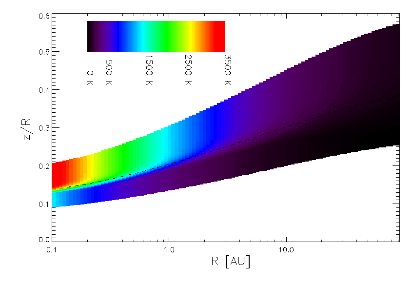
Figure 18: The temperature structure of a flared-disk model. On the x-axis the radial distance $R$ to the star is plotted, on the y-axis the ratio of the height above the midplane $z$ over $R$. The color scale is linear and ranges from 0 to 3500K. The dashed line represents the disk surface height $H_{cg}$.

We note that the temperature stratification in the disk and the density function are not computed self-consistently. The temperature gradient is calculated a posteriori; the effect of the higher temperatures in the upper layers of the disk is not included in the determination of $\rho$. The deviation from the self-consistent calculation is however very small.

5.2 The [O i] emission

To determine the [O i] 6300Å emission emanating from a flared circumstellar disk, we have implemented the model of Störzer & Hollenbach (2000) for [O i] emission. They have modelled the optical forbidden-line emission from a plane-parallel semi-infinite photodissociation region (PDR). Both thermal and non-thermal emission are included. Slight changes were applied to the method to adapt it to our specific case.

5.2.1 Thermal [O i] emission

Following Störzer & Hollenbach (2000), a five-level oxygen atom is assumed. The atomic data and references can be found in their paper (Table 1 of the Appendix). Since we are only interested in modeling the 6300Å line, the relevant transitions for the present paper are ${{}^{3}P_{1}}\longrightarrow{{}^{3}P_{2}}$ (63.2 $\mu$m), ${{}^{3}P_{0}}\longrightarrow{{}^{3}P_{2}}$ (44.2 $\mu$m), ${{}^{1}D_{2}}\longrightarrow{{}^{3}P_{2}}$ (6300.3Å) and ${{}^{1}S_{0}}\longrightarrow{{}^{1}D_{2}}$ (5577.4Å). Collisions with free electrons and atomic hydrogen are considered. From PDR models (e.g. Hollenbach & Tielens 1999, and references therein), one derives that the transition region from the atomic-H dominated upper layers to the disk interior where H₂ is abundant occurs at about $A_{V}=1$. Based on the latter, we assume that only at $A_{V}<1$ free electrons and H atoms are important collisional partners for the O i atom. In optically thick regions, the collisional rate is set to zero.

The proton number density $n_{p}$ depends on the radial and vertical position $(R,z)$ in the disk and the input surface density $\Sigma$. It is computed from the flared-disk model. The oxygen number density is the product of the proton density and the fractional oxygen abundance

$$n(O)=n_{p}\left[\frac{O}{H}\right].$$ (4)

A typical interstellar value for $[O/H]$ is $5\times 10^{-5}$ (e.g., Allen 1976). In the region where oxygen is not ionized, the atomic hydrogen is neutral as well, because the ionization energy of the two species is comparable. In this region the free electrons are almost all due to the ionization of neutral carbon atoms. Assuming all carbon atoms in the considered region are singly ionized, the free-electron number density is

$$n_{e^{-}}=n_{C^{+}}=n_{p}\left[\frac{C}{H}\right].$$ (5)

A typical interstellar fractional abundance of carbon is $3\times 10^{-4}$.

To determine the thermal [O i] 6300Å emission, the population of the upper level of this line (${}^{1}D_{2}$) needs to be known. Using the formula of thermal equilibrium (see Appendix), one can determine the relative population of two levels $a$ and $b$ for a temperature $T$. From the latter ratios, the relative fraction $F$ of O i atoms in the ${}^{1}D_{2}$ state can be calculated. The number density of the thermally populated upper level of the 6300Å line is $n_{u,th}=F\,n(O)$.

Since the typical temperature range (10–1500K) in our disk models is rather low to thermally excite the oxygen atoms, the emanating [O i] 6300Å emission is very weak. The intensity of the thermal emission is more than a million times smaller than the non-thermal [O i] emission, which is discussed in the next section.

5.2.2 Non-thermal [O i] emission

Following Störzer & Hollenbach (2000), the dominant non-thermal excitation mechanism for neutral oxygen atoms is the photodissociation of OH molecules. This results in a hydrogen atom and an excited oxygen atom. A fraction of the latter ($\sim$55%, van Dishoeck & Dalgarno 1984) find themselves in the upper state (${}^{1}D_{2}$) of the 6300Å line. This mechanism hence produces strong non-thermal [O i] emission in regions where the photodissociating UV flux is abundant and the densities high enough to have a sufficient amount of emitting oxygen atoms.

In our simple model for non-thermal emission, we assume that the fractional OH abundance $\epsilon(OH)$ is constant throughout the disk. In reality, this may not be the case, as the optically thick disk interior will have a much higher $\epsilon(OH)$ than the photon-immersed surface layers. Nevertheless this assumption needs not to be valid for the entire disk, but only for the [O i] emission region. The latter will be located close to the $\tau=1$ surface and is geometrically quite thin, because the proton density drops off rapidly when moving away from the disk midplane while the high optical depth in the disk interior prohibits photodissociation of the OH molecules. From the OH number density $n(OH)=\epsilon(OH)\times n_{p}$, the density of non-thermally-excited oxygen atoms can be determined (Störzer & Hollenbach 1998, adapted to the UMIST rate coefficients):

$$n_{u,non-th}=f\,G_{0}\,\frac{3.50\times 10^{-10}}{A}\,e^{-1.7A_{V}}\,n(OH).$$ (6)

7 In this formula, $f$ ($\approx$ 55%) is the fraction of oxygen atoms released by the photodissociation of OH in the upper level of the 6300Å line. The sum ($A$) of the Einstein transition rates from the ${{}^{1}D_{2}}$-level downwards is approximately $8.4\times 10^{-3}$ s^-1 (Osterbrock 1989).

The local [O i] 6300Å emissivity $j(R,z)$ (in erg s^-1 cm^-3 sr^-1) is given by

$$j(R,z)=\frac{1}{4\pi}h\nu\ A_{6300}n_{u}(R,z)$$ (7)

The Einstein coefficient $A_{6300}$ is $6.3\times 10^{-3}$ s^-1 (Osterbrock 1989). The value $h\nu$ is the energy of a 6300Å photon. The density $n_{u}$ is the sum of the densities of the thermally and non-thermally excited oxygen atoms. In Fig. 19, $j(R,z)$ is plotted as a function of the vertical and radial location in the disk. The dashed line represents the disk surface height $H_{cg}$ of the disk. The emission is located around this region.

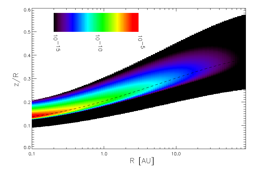
Figure 19: The [O i] 6300Å emissivity in the flared-disk model. The x-axis gives the radial distance $R$ to the central star in AU, the y-axis plots $z/R$, the ratio of the vertical height and the radial distance. The colors represent the local [O i] 6300Å emissivity on a log-scale which covers 10 orders of magnitude. On the color bar, the emissivity is given in [erg s^-1 cm^-3 sr^-1]. The disk region sampled by the model ranges from roughly 0.6 to 1.5 times the disk surface height $H_{cg}$. The latter is indicated by the dashed line. The geometrical full width at half maximum of the [O i] emission region in the vertical direction is 5–10% of $H_{cg}$.

Integrating the emissivity over the vertical direction, considering the optical depth $\tau_{6300}$ at 6300Å, one extracts the surface intensity $I(R)$ at each radius $R$:

$$I(R)=\int_{z}j(R,z)\,e^{-\tau_{6300}}dz$$ (8)

The unit of $I(R)$ is erg s^-1 cm^-2 sr^-1. Note that, due to the shallow angle under which the stellar light impinges on the disk, one looks much deeper into the disk in the vertical than in the radial direction. When looking at the disk face-on, the observer practically sees the entire [O i] emitting region (on one side of the disk).

5.3 The line profiles

To convert the intensity-versus-radius function $I(R)$ to an intensity-versus-velocity profile, we assume that the rotation of the disk is Keplerian. We anticipate this to be a fairly accurate assumption, since the disk mass is expected to be much smaller than the mass of the central star (e.g., Acke et al. 2004). Additionally we adopt that the Keplerian rotation velocity of matter in the upper layers of a flared disk is the same as the rotational velocity in the midplane. Fig. 20 illustrates how the profile is computed. The light-grey band in the pictogram represents a circular orbit in the inclined –geometrically flat– disk where the [O i] intensity is constant. The disk’s matter in this band rotates around the central star with a Keplerian velocity $v_{\mathrm{kep}}=\sqrt{GM_{\star}/R_{\mathrm{orbit}}}$ in which $R_{\mathrm{orbit}}$ is the radius of the orbit and $M_{\star}$ is the mass of the central star. The narrow darker-grey band represents the parts of the disk that move towards (or away from) the observer with the same projected velocity $v_{\mathrm{proj}}$. This area is the region where

$$R=\frac{GM_{\star}}{v_{\mathrm{proj}}}\sin^{2}i\,\sin^{2}\theta$$ (9)

with $\theta$ the angle in the disk plane ($\theta=0^{\circ}$ towards the observer). The inclination $i$ is defined to be $0^{\circ}$ for pole-on disks. The black surface is the cross-section of both bands. By adding up these regions and multiplying with the intensity, the intensity-versus-velocity profile is built up for each projected (=observed) velocity.

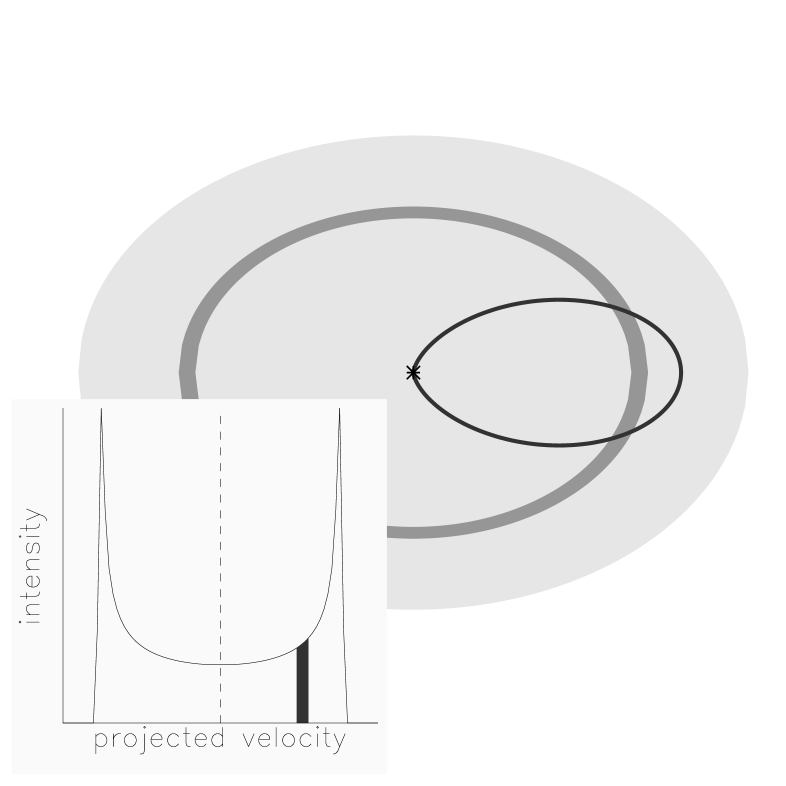
Figure 20: Pictogram of a flat rotating circumstellar disk, seen under an inclination of $i=45^{\circ}$. The location of the central star is indicated by the asterisk. The light-grey band represents a circular orbit. In this orbit, the rotational velocity as well as the [O i] intensity (I_o) are constant due to the assumption of axisymmetry. The narrow dark-grey band represents the region where the projected rotational velocity is equal to a certain value $v_{p}$. At the cross-section of both surfaces the projected velocity is equal to $v_{p}$ and the intensity is equal to I_o. The insertion shows the intensity-versus-velocity profile of the light-grey band. The dark-grey part represents the contribution of the cross section of the dark-grey band and the orbit in the disk.

The computed theoretical profile is then convolved with a Gaussian function. This function mimics the effect of instrumental broadening. The width of the –unresolved– telluric lines in each type of spectrum were used as the width of the instrumental Gaussian profile.

5.4 Discussion of the model parameters

The input parameters for our model that calculates the non-thermal emission consist of some stellar parameters ($L_{\star},L_{\mathrm{uv}},M_{\star},T_{\star}$) which are derived from the photometric data. Furthermore, a dust opacity table and dust-to-gas mass ratio are needed. Following the Dullemond et al. (2001) model for AB Aur, we assume that the dust consists of olivines and represents 1% of the total disk mass. The stellar parameters are $L_{\star}=47\leavevmode\nobreak\ L_{\odot}$, $L_{\mathrm{uv}}=36\leavevmode\nobreak\ L_{\odot}$, $M_{\star}=2.4\leavevmode\nobreak\ M_{\odot}$ and $T_{\star}=9520$K. The free parameters in our [O i] emission model are the surface density $\Sigma=\Sigma_{0}\,(R[AU])^{-\beta}$, the fractional OH abundance $\epsilon(OH)$ and the disk’s inclination $i$. In the template model, we take $\Sigma_{0}=10^{4}$ g cm^-2, $\beta=2$, $\epsilon(OH)=1\times 10^{-6}$ and $i=45^{\circ}$. The inner and outer radius of the disk, $R_{in}$ and $R_{out}$, are 0.1 AU and 100 AU respectively. We discuss the influence of the four free input parameters on the shape of the emission profile, starting with the surface density.

The two parameters $\Sigma_{0}$ and $\beta$ describing the power-law surface density are coupled when the disk mass is known:

$$M_{disk}=2\pi\int_{R_{in}}^{R_{out}}\Sigma_{0}\,R^{1-\beta}dR$$ (10)

The disk mass of our template model is $M_{disk}=0.049M_{\odot}$. In Fig. 21, the intensity-versus-radius distribution of the [O i] 6300Å emission is plotted for four models. The input parameters of the latter are the template values, except for $\Sigma$. The power $\beta$ ranges from 1.0 to 3.0, while $\Sigma_{0}$ is appropriately adapted to ensure that the disk mass remains unaltered. The total emission intensity decreases with increasing $\beta$. Fig. 22 shows the line profiles, corresponding to the intensity distributions in Fig. 21.

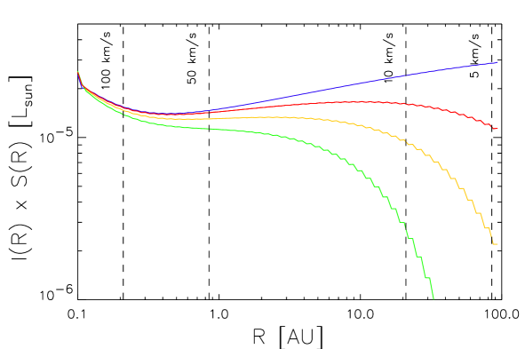
Figure 21: The intensity-versus-radius distribution $I(R)$ for four template models, with different values for the surface-density parameters. From top to bottom, $\beta$ is 1.0, 2.0, 2.5 and 3.0 respectively. The value of $\Sigma_{0}$ is chosen such that the disk masses of the four models are the same. The intensity function is multiplied by the total surface $S(R)$ of the ring at radius $R$. In this way the fluxes from the inner and outer parts of the disk can be compared directly. The vertical dashed lines mark the radii where the Keplerian velocity is 5, 10, 50 and 100 $\mathrm{km}\leavevmode\nobreak\ \mathrm{s}^{-1}$. The shoulder of the intensity distribution shifts closer to the star with increasing $\beta$. Furthermore, the total emission is smaller when the power-law describing $\Sigma$ has a steeper slope.

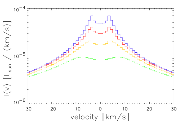
Figure 22: The line profiles $I(v)$ corresponding to the intensity-versus-radius distribution in Fig. 21. From top to bottom, $\beta$ is 1.0, 2.0, 2.5 and 3.0 respectively. Since the intensity-versus-radius distribution falls off rapidly in the models with large $\beta$ values, the corresponding profiles have peaks at higher velocities than the profiles belonging to low-$\beta$ models.

The fractional OH abundance $\epsilon(OH)$ scales linearly with the total intensity of the profile. It does not alter the shape, as we assume it is constant throughout the [O i] emission region.

Observations of Doppler-broadened spectral lines do not observe the real, but the projected velocities in the system. In the present flared-disk model, the inclination $i$ is a free parameter which alters the shape as well as the intensity of the computed profile. The total integrated intensity $\int I(v)dv$ is proportional to $\cos i$, while the position of the two typical peaks of the line changes with $\sin i$. Fig. 23 shows the line profiles of the template model as seen under different inclinations. Note that inclinations larger than about $70^{\circ}$ are not relevant in flared disks, since at such high $i$, the outer parts of the disk would occult most of the disk surface.

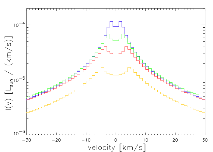
Figure 23: The line profiles $I(v)$ of the template model seen under different inclinations. From top to bottom, the inclination is $18^{\circ},30^{\circ},45^{\circ}$ and $70^{\circ}$ respectively. Note the decrease in integrated intensity and the shift of the peaks with increasing $i$.

6 Comparison with the observations

In this section we compare our model results to the observations. We focus on the sample stars which display a narrow, symmetric and centered profile. Since the thermal emission is weak compared to the non-thermal emission for the relatively cool disks studied in this paper, we will only consider the non-thermal emission component in the following discussion.

Figure 24: Similar plot as Fig. 12. The filled diamonds are the observed [O i] intensities for the group I sources. The open circles represent model results. The typical error bar for the observations is given in the upper left corner. The models differ from each other in stellar parameters; from the lower left to the upper right, the model [O i]-versus-UV luminosity for a typical F0V, A3V, A0V, B8V, B5V and B0V star are plotted respectively. The error bars on the model determinations represent the spread in results when simultaneously varying the surface density $\Sigma$ and inclination $i$ in the ranges described in Figs. 22 and 23. The dotted lines represent the model results when altering the fractional OH abundance $\epsilon(OH)$ and using the average [O i]-versus-UV luminosity ratio of the models. The abundance is indicated next to each line, with $a(-b)$ representing $a\times 10^{-b}$. The fractional OH abundance of the models is $1\times 10^{-6}$.

We compare the observed [O i] 6300Å emission luminosity and its theoretical counterpart to the UV luminosity in Fig. 24. Our model applies for flared-disk geometries, therefore only the group I sources have been plotted in the figure. The model results and the observations agree nicely for an acceptable range of the free parameters $\Sigma$, $i$ and $\epsilon(OH)$. Note that all models in the figure have the same disk mass as the template model. Varying the disk mass affects the [O i] 6300Å emission in a comparable manner as when the surface density is altered. Fig. 25 compares the [O i] luminosity to the effective temperature of the group I objects and the models. Again, reasonable values for the free parameters lead to theoretical [O i] luminosities close to the observed values.

Figure 25: The [O i] 6300Å luminosity versus the effective temperature of the group I sources (filled diamonds). The open circles and dotted lines plotted in this figure represent the same models as in Fig. 24.

Not only the strength of the [O i] 6300Å emission can be reproduced with our model. After scaling the total theoretical to the observed intensity, the typical FWHM and double-peaked shape of the narrow centered features can be explained by assuming Keplerian rotation of the flared disk. In Fig. 26 we have overplotted observed profiles with theoretical ones. For each star, we have used the stellar parameters ($L_{\star},T_{\star},M_{\star}$) as input parameters. The remaining parameters were set to the template values, unless otherwise indicated in the plots. Note that the theoretical profiles are not fitted to the data, but are just overplotted model profiles, rebinned to the spectral resolution of the observed spectrum. The similarity between theory and observation is nevertheless striking. For AB Aur and HD 100546, the inclination of the disk have been determined to be $i=76^{\circ}$ (Mannings & Sargent 1997) and $i=51^{\circ}$ (Augereau et al. 2001) respectively. The observed profiles of the [O i] 6300Å line can be approximated by theoretical line profiles for these inclinations when using $\epsilon(OH)\approx 2\times 10^{-6}$ and $\beta=1.5$ for AB Aur and $\epsilon(OH)\approx 6\times 10^{-7}$ and $\beta=2.5$ for HD 100546.

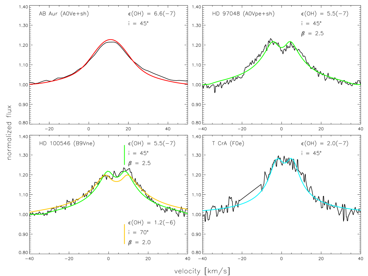
Figure 26: The observed spectra of group I sources AB Aur, HD 97048, HD 100546 and T CrA overplotted with the model results. The parameters of the model are adapted to the stellar parameters of each source combined with the template parameters, unless otherwise indicated in the upper right corner. We have shifted the theoretical profile to the centroid position of the observed feature. For HD 100546 two models with different parameter sets have been displayed to illustrate the difficulty to distinguish between models. The theoretical profiles extracted from our flared-disk model fit the observed features strikingly well for a range of reasonable model parameters. $a(-b)$ represents $a\times 10^{-b}$.

The flaring of the disk is due to the dust opacities, while the gas opacities are negligible. Since dust evaporates above the dust sublimation temperature $T_{subl}\sim 1500$K, we have shifted the inner edge of the flared-disk from $R_{in}=0.1$ AU to the radius where the surface temperature $T_{s}$ equals $T_{subl}$. For a typical F0V, A0V and B0V star, the inner radius hence becomes 0.2, 0.8 and 30 AU respectively. As a consequence, the high-velocity ($|v|\gtrsim$ 50 $\mathrm{km}\leavevmode\nobreak\ \mathrm{s}^{-1}$) wings of the theoretical [O i] emission line profile disappear, in agreement with the observed spectra of narrow 6300Å features which do not display extended wings (e.g., AB Aur, HD 97048, HD 100546, HD 135344, HD 169142, R CrA, T CrA, HD 179218, HD 190073). Furthermore, the models of Dullemond (2002) suggest that the inner rim of the disk is puffed-up and casts its shadow of the first few AU in a flared geometry. This effect could be mimicked in our flared-disk model by shifting the inner radius $R_{in}$ even further out (up to $\sim$5 AU). The effect of the latter on the theoretical line profile would be mostly a decrease of the wings, without reducing the total intensity much.

The innermost parts of the circumstellar disk, where no dust can survive due to the high temperatures, are relatively small in spatial dimensions. Nevertheless, we cannot exclude that the contribution of these parts to the total [O i] emission strength is significant. Specifically, a few group II sources (e.g., VX Cas, V586 Ori, HD 95881, HD 98922, HD 101412, WW Vul, SV Cep) display broader, but relatively weaker [O i] profiles. In our current interpretation and with no external bright UV source near, this [O i] emission cannot emanate from the disk surface for the self-shadowing prohibits direct stellar flux to reach this area. In the latter cases, the emission might come from a rotating gaseous disk inside the dust-sublimation radius. The modeling of this inner gaseous region is however beyond the scope of the present paper. We refer to the recent paper of Muzerolle et al. (2004) for a more elaborate discussion on this subject.

7 Conclusions and discussion

The observed [O i] 6300Å emission line in many HAEBE stars in our sample shows evidence for a rotating forbidden-line emission region. In this paper we suggest that the surface of the flared circumstellar disk around the group I objects is the perfect location to harbor this emission region. The combination of the direct stellar UV flux and the relatively high densities in this region give rise to strong non-thermal [O i] emission, which can explain the observed luminosities reasonably well. Furthermore, the shape of the spectrally resolved 6300Å profile in the observations and the profile produced by our simple model indicate that Keplerian rotation indeed is the broadening mechanism for (at least the narrow component of) this line. The observed 6300Å spectra of the group I members in our sample can be reproduced strikingly well.

In the group of self-shadowed-disk sources, significantly more targets do not display the [O i] 6300Å emission line (43% versus 8% in group I). The line profiles of the detected [O i] 6300Å emission feature in group II are twice as weak as, and somewhat broader than the lines observed in group I spectra. In our current interpretation, the surface of a self-shadowed disk’s outer parts is not directly irradiated by the central star. However, the non-thermal [O i] line formation mechanism —photodissociation of OH and H₂O— may produce the observed group II emission lines as well. Assuming that the [O i] emission emanates from the inner gaseous disk naturally explaines the weaker emission and the higher-velocity wings of the feature: the inner gaseous disk provides a smaller emission volume and is located closer to the central star, where the Keplerian velocities are larger.

In T Tauri stars, the less massive counterparts of HAEBE stars, the observed [O i] emission profile can be explained using the model of Kwan & Tademaru (1988) (e.g. Hartigan et al. 1995). However, this model assumes that a “super-heated” disk atmosphere, fed by accretion, is present, in which the temperatures are sufficiently high ($\sim$10⁴K) to produce thermal [O i] emission. The absence of a strong UV excess and strong photospheric veiling, the relatively weak IR recombination lines and CO emission, and the presence of 10 micron silicate emission (AV04) in the majority of the group I and II sources in our sample all indicate that these disks are passive. Furthermore, the observed upper limits for the 5577/6300 [O i] ratio indicate that the observed emission cannot be thermal. Each model which models the [O i] emission based on thermal processes —including the disk wind model— will have difficulties reproducing the strength of the [O i] 6300Å line in HAEBE stars. The non-detections of the [S ii] 6731Å line in the spectra of group I and II sources in our sample confirm this picture. Moreover, amongst the late-type sample sources no strong [O i] emitters are present. In the T Tauri model the forbidden line emission is dependent on accretion rate and thus the model cannot explain the absence of strong late-type [O i] sources. The OH photodissociation model suggested in the present paper naturally predicts that passive disks around weak UV sources will not produce strong [O i] 6300Å emission.

The high-velocity blue wings in the [O i] 6300Å line of a small minority of our sample stars cannot be accounted for by an emitting passive Keplerian disk. This emission feature is suggested to emanate from an outflow, of which the redshifted part is occulted by the circumstellar disk. Note however that this pronounced blue wing is often accompanied by a symmetric peak at low velocities (e.g., Z CMa, PV Cep, V645 Cyg, HD 200775). The latter might again be formed in the surface layers of the rotating disk. Alternatively, the model of Kwan & Tademaru (1988) for T Tauri stars may be valid for these objects: since the assumption of passivity is likely not to be valid for the disks of the group III members, these sources might resemble classical accreting T Tauri stars. As noted before, accretion is needed to create the right settings for the T Tauri model to work. This idea is supported by the detection of the [S ii] 6731Å line in Z CMa, which is exclusive to this target in the present sample. We note however that this behaviour seems to be rather exceptional for HAEBE stars.

The values for the fractional OH abundance $\epsilon(OH)$ needed to explain the observed [O i] 6300Å luminosities are $\sim$10${}^{-7}-10^{-6}$. Observations of diffuse interstellar clouds show that relative OH abundances of this magnitude ($\sim$10^-7) occur in the interstellar medium (e.g., Crutcher 1979, and references therein). Nevertheless, these values are two orders larger than the abundances computed in recent models including a full treatment of disk chemistry (e.g., Markwick et al. 2002; Kamp & Dullemond 2004). A possible reason for this discrepancy may be the exact location of the [O i] emission region in our models: a shift to higher densities (i.e. to a lower vertical height $z$) would reduce the fractional OH abundance required to fit the observed [O i] intensity, since the latter is inversely proportional to the first. This effect can potentially be induced by the input dust opacities, which define the disk’s flaring, but also the UMIST coefficients determine the exact location of the [O i] emitting region through formula (6). Alternatively, the chemical models may be wrong due to uncertainties in the reaction rate coefficients or the incompleteness of the network.

Böhm & Hirth (1997) have stated that the forbidden-line emission region in Hillenbrand et al. (1992) group I sources cannot be located at the surface of the circumstellar disk, because the suggested accretion disk would cover most of the forbidden-line emission region. The authors suggest that, even when the stellar light is able to reach the disk surface, a problem remains: the upper layer would be geometrically very thin and the outer radius of the disk would need to be much larger than 100 AU in order to create enough emission volume to explain the observed [O i] intensities. Both problems are countered when considering a flared disk with a puffed-up inner rim. Hillenbrand et al. have invoked a circumstellar accretion disk model to explain the observed near-IR ($\sim$2 $\mu$m) bump which is typical for Hillenbrand group I sources. The puffed-up inner rim in the Dullemond et al. (2001) model naturally explains this excess. In other words, no dynamically active model is needed to explain this bump. Furthermore, the outer parts of the disk can be flared, hence increasing the angle $\alpha$ under which the stellar light impinges onto the disk surface. The UV flux can penetrate deeper into the disk, thus increasing the geometrical thickness of the [O i] emission layer. As we have shown in the present paper, the observed [O i] 6300Å emission profile can be explained as being due to the photodissociation of OH molecules and the subsequent non-thermal excitation of oxygen atoms in the atmosphere of a rotating flared disk.

Appendix

The fractional level population of two levels $a$ and $b$ of an atom in thermal equilibrium at a temperature $T$[K] is given by

$$\frac{N_{b}}{N_{a}}=\frac{g_{b}}{g_{a}}\frac{1}{1+\frac{A_{ba}}{n\gamma_{ba}}}\exp\left(-\frac{E_{ba}}{T}\right)$$ (11)

In this formula, $g_{a}$ and $g_{b}$ are the statistical weights, $A_{ba}$ is the Einstein transition rate for the transition between level $b$ and $a$ and $E_{ba}$ is the energy of the transition in K. The factor $n$ is the number density of the collisional partner, $\gamma_{ba}$ is the collisional rate for the transition and the collisional partner. When more than one collisional partner is involved, the quantity $n\gamma_{ba}$ is equal to the sum of these values for each interacting species $i$: $n\gamma_{ba}=\Sigma_{i}\,n_{i}\,\gamma_{ba}^{i}$.

To determine the fraction $F$ of neutral oxygen in the ${}^{1}D_{2}$ state in the five-level model assuming thermal excitation, one applies

$$F=\left(\frac{\Sigma_{j=1}^{5}N_{j}}{N_{{}^{1}D_{2}}}\right)^{-1}=\left(\Sigma_{j=1}^{5}\frac{N_{j}}{N_{{}^{1}D_{2}}}\right)^{-1}$$ (12)

These ratios can easily be computed using equation (11), the atomic data and the fact that

$$\frac{N_{a}}{N_{b}}=\left(\frac{N_{b}}{N_{a}}\right)^{-1}$$ (13)