Orbital modulation of emission of the binary pulsar J0737-3039B

Abstract

In binary radio pulsar system J0737$-$3039, slow pulsar B shows orbital modulations of intensity, being especially bright at two short orbital phases. We propose that these modulations are due to distortion of pulsar B magnetosphere by pulsar A wind which produces orbital phase-dependent changes of the direction along which radio waves are emitted. In our model, pulsar B is intrinsically bright at all times but its radiation beam misses the Earth at most orbital phases. We employ a simple model of distorted B magnetosphere using stretching transformations of Euler potentials of dipolar fields. To fit observations we use parameters of pulsar B derived from modeling of A eclipses (Lyutikov & Thompson 2005). The model reproduces two bright regions approximately at the observed orbital phases, explains variations of the pulse shape between them and regular timing residuals within each emission window. It also makes predictions for timing properties and secular variations of pulsar B profiles.

1 Introduction

Double pulsar system PSR J0737$-$3039A/B contains a recycled 22.7 ms pulsar (A) in a 2.4 hr orbit around a 2.77 s pulsar (B) (Burgay et al., 2003; Lyne et al., 2004). Emission of pulsar B is strongly dependent on orbital phase. It is especially bright at two windows, each lasting for about $30^{\circ}$. One of the emission windows appears near superior conjunction (when pulsar B is between pulsar A and observer), and another approximately $70^{\circ}$ before it. Pulse profiles have different shapes in the two windows. In addition, Ransom et al. (2004a) have detected regular, orbital phase-dependent drift of emission arrival times by as much as 20 ms.

Previously, Jenet & Ransom (2004) suggested that emission of B is initiated by $\gamma$-ray emission from A. This model seems to be inconsistent with the evolution of the A profile (Manchesteret al. , 2005). Zhang & Loeb (2004) suggested that B emission is triggered by particles from pulsar A wind reaching deep into magnetosphere. This model is incorrect since the authors neglected magnetic bottling effect, which would reflect most pulsar A wind particles high above in B magnetosphere (see Lyutikov & Thompson, 2005, for discussion of particle dynamics inside B magnetosphere)

In this paper we explore an alternative possibility that orbital brighting of B is due to distortions of B magnetosphere by pulsar A wind. We show that due to orbital phase-dependent distortions of B magnetosphere, the polar magnetic field lines, along which emission is presumably generated, may be “pushed” in the direction of an observer at particular orbital phases, while at other moments radiating beam of B misses the observer.

2 Distortion of pulsar B magnetosphere

Magnetosphere of pulsar B is truncated, if compared to magnetosphere of an isolated pulsar of the same spin, by the relativistic wind flowing outward from pulsar A. The size of magnetosphere is $R_{m}\sim 4\times 10^{9}$ cm (Lyutikov, 2004; Arons et al., 2004; Lyutikov & Thompson, 2005), which is 3 times smaller than the light cylinder radius $R_{LC}=\Omega/c=1.3\times 10^{10}$ cm ($\Omega$ is angular frequency of pulsar B rotation, $c$ is velocity of light). At intermediate distances, $R_{NS}\leq r\leq(R_{LC},\,R_{m})$, neutron star magnetospheres are well approximated by dipolar structure. This has been a longstanding assumption in pulsar theory (Goldreich & Julian, 1969), and has recently been confirmed by modeling of pulsar A eclipses (Lyutikov & Thompson, 2005).

A small degree of distortion of magnetosphere from the dipolar shape is expected at intermediate distances due to several types of electrical currents. First, distortions are due to confining Chapman-Ferraro currents (Chapman & Ferraro, 1930) flowing in the magnetopause (a region of shocked pulsar A wind around B magnetosphere). At the emission radius, $R_{em}\sim 1-5\times 10^{8}$ cm (see below), fractional distortions due to Chapman-Ferraro currents are expected to be small $\sim(R_{em}/R_{m})^{3}\sim.001-.02$. In addition to confinement of magnetosphere on the side facing pulsar A (“dayside”), on the side opposite to pulsar A (“nightside”) magnetosphere of B extends to large distances, somewhat similar to the Earth magnetosphere under the influence of Solar wind. Secondly, similar to isolated pulsars, there are conduction Goldreich-Julian currents, arising on the open field lines due to relativistic electromagnetic effects of rotation, and displacement currents, arising in oblique rotators due to temporal variations of electromagnetic fields. At the emission radius these currents produce a distortion of magnetic field of the order $\sim(R_{em}/R_{LC})^{2}\sim 10^{-3}$. Thirdly, there are internal currents flowing in the magnetosphere, like ring current, Birkland currents, and other types of currents.

Clearly, the detailed structure of pulsar B magnetosphere is even more complicated than that of the Earth, but at distances from the star smaller than light cylinder and magnetospheric radii distortions from dipolar form are expected to be small. This should be the case in the emission generation region. In addition, since magnetospheric radius $R_{m}$ is several times smaller than light cylinder we can make a simplifying assumption that at each given moment the structure of the inner magnetosphere is determined by the instantaneous direction of the magnetic moment of B and the direction of line connecting two pulsars (which is, approximately, the direction of pulsar A wind at the position of B). Under this approximation we expect that at each moment the structure of the inner magnetosphere may be estimated using methods developed for non-relativistic, quasi-stationary magnetospheres of solar planets interacting with the solar wind. This interaction is complicated, depending on a number of both macroscopic (e.g. wind pressure, direction of magnetic field, dipole inclination) and especially microscopic (e.g. reconnection and diffusion rates) parameters. In what follows we use experience with the solar wind – Earth magnetosphere interaction (e.g.  Tsyganenko, 1990) as a guiding line in studying pulsar B magnetosphere.

One of the principal issues here is how magnetopause currents respond to the dipole magnetic field of the central object. Two extreme possibilities are (i) complete screening of the dipole, so that no pulsar magnetic field lines penetrate into the wind and (ii) efficient reconnection so that most of the pulsar magnetic field lines that reach the magnetospheric boundary penetrate into the wind. In the case of the Earth magnetosphere, though reconnection plays an important role, on average inter-penetration of magnetic field is at most a $10\%$ effect (eg. Stern, 1987). (Rates of reconnection are strongly dependent on the direction of the solar wind magnetic field. On the dayside reconnection occurs most efficiently near the cusps, where polar magnetic field lines reach magnetopause.) Numerical modeling of interaction of relativistic pulsar A wind with pulsar B shows qualitatively similar results Arons et al. (2004). Thus, as a first approximation, we may assume that magnetopause currents screen out pulsar B magnetic field.

An additional source of magnetic field distortion is the ring current generated by particles trapped inside magnetosphere. Modeling of pulsar A eclipses (Lyutikov & Thompson, 2005) implies that high density, relativistic plasma (most likely composed of pairs) is present on closed field lines of pulsar B. In addition to bouncing between magnetic poles due to effect of magnetic bottling, trapped particles drift along magnetic equator. Viewed from the north magnetic pole, positrons drift clockwise, electrons – counterclockwise, producing a ring current, which modifies the structure of magnetosphere. We expect that effects of the ring current are negligible at the emission radius. A typical drift velocity of charge carries is $u_{d}\sim c^{2}\gamma_{0}/\omega_{B}R_{m}\sim 3\times 10^{4}$ cm/sec (here $\gamma_{0}\sim 10$ is a typical Lorentz factor of trapped particles, $\omega_{B}$ is cyclotron frequency). For particle density $n\sim\lambda_{m}n_{GJ,m}$ ($n_{GJ,m}$ is Goldreich-Julian density at the magnetospheric radius $R_{m}=4\times 10^{9}$ cm and $\lambda_{m}$ is multiplicity factor at $R_{m}$), the current density is $j\sim\lambda_{m}n_{GJ,m}u_{d}e\sim.1j_{GJ}$, and total current is $I\sim jR_{m}^{2}$. Resulting magnetic field is $B_{ring}\sim I/(R_{m}c)\sim jR_{m}/c\sim\lambda_{m}(\Omega R_{m}/c)(u_{d}/c)B_{m}\sim.03B_{m}$. Deep inside magnetosphere, the magnetic field of the ring current is nearly constant, but the dipole field increases, so that at $R_{em}\sim 10^{8}$ cm $B_{ring}/B_{d}\sim 10^{-5}$. (Qualitatively, the magnetic field of the ring current would become comparable to the dipole field at $R_{m}$ when energy density of trapped plasma is of the order of magnetic field energy density.)

There are other types of currents that can modify field structure like Birkland and tail currents (e.g.  Tsyganenko, 1990). Their influence on the structure of magnetosphere at intermediate distances is expected to be small and we neglect them here. Thus, we assume that the only currents contributing to the distortion of magnetosphere are magnetopause Chapman-Ferraro currents which screen pulsar B field. This simplification allows us to use models developed for the Earth magnetosphere in order to estimate distortions of pulsar B magnetic field.

3 Modeling distorted magnetosphere of B

There is extensive literature on modeling of the Earth magnetic field (e.g.  Tsyganenko, 1990). A number of analytical methods have been developed. For our purposes, we do not need to calculate the full structure of magnetosphere, but only to estimate variations in the position of polar magnetic field lines, where emission of B is presumably generated. For this purpose we employ the method of distortion transformation of Euler potentials (Stern, 1994; Voigt, 1981). A major advantage of the stretching model of magnetosphere is that it reproduces fairly well the structure of a tilted dipole (Stern, 1994).

Magnetic field can be described by two Euler potentials $\alpha$ and $\beta$ (sometimes called Clebsch potentials):

$${\bf B}=\nabla\alpha\times\nabla\beta$$ (1)

so that magnetic field line is defined by an intersection of surfaces with constant $\alpha$ and $\beta$. Magnetosphere of B enshrouded by magnetopause resembles a dipole field compressed on the dayside and stretched out on the nightside. The structure of the nightside magnetosphere can be approximated by stretching transformations of the Euler potentials $\alpha$ and $\beta$.

Let us choose a system of Cartesian coordinates in the tail of B magnetosphere, centered on pulsar B so that $z^{\prime}$ axis is along the line connecting pulsar A and B and axis $x^{\prime}$ is in the ${\vec{\mu}}-z^{\prime}$ plane, where ${\vec{\mu}}$ is magnetic moment of B, see Fig. 1. Let the magnetic dipole be inclined at angle $\theta_{\mu}$ to axis $z^{\prime}$. The undistorted dipole Euler potentials are

$$\alpha_{0}=R_{NS}\mu{(-x^{\prime}\sin\theta_{\mu}+z^{\prime}\cos\theta_{\mu})^{2}+y^{\prime 2}\over\sqrt{x^{\prime 2}+y^{\prime 2}+z^{\prime 2}}}\mbox{}$$

$$\beta_{0}=R_{NS}\arctan{y^{\prime}\over-x^{\prime}\sin\theta_{\mu}+z^{\prime}\cos\theta_{\mu}}$$ (2)

Stretching transformations along $z^{\prime}$ axis are defined by potential $f(z^{\prime})$, so that new Euler potentials are expressed in terms of dipolar ones: $\{\alpha,\beta\}=\{\alpha_{0}(z^{\prime}=f(z^{\prime})),\beta_{0}(z=f(z^{\prime}))\}$. A degree of stretching depends on $f^{\prime}(z^{\prime})$. In modeling of the Earth magnetosphere function $f(z^{\prime})$ is chosen to fit satellite data. Since we are interested in the distortions at one particular location (assuming that radio emission is generated in a narrow range of radii), we choose $f^{\prime}(z^{\prime})=C=$const $<1$, similar to Voigt (1981) model of Earth magnetosphere. Thus, $C$ measures the distortion of magnetosphere at the emission radius.

Substituting $z^{\prime}\rightarrow Cz^{\prime}$ in Eq. (2) we find stretched magnetic fields in coordinates $\{x^{\prime},y^{\prime},z^{\prime}\}$

$${\bf B}={r_{0}^{3}\mu\over\tilde{r^{\prime}}^{5}}\left\{3Cx^{\prime}z\cos\theta_{\mu}+(2C^{2}x^{\prime 2}-y^{\prime 2}-z^{\prime 2})\sin\theta_{\mu},\right.\mbox{}$$

$$3y^{\prime}C(z^{\prime}\cos\theta_{\mu}+Cx^{\prime}\sin\theta_{\mu},\mbox{}$$

$$\left.C\left(3Cx^{\prime}z^{\prime}\sin\theta_{\mu}+(2z^{\prime 2}-C^{2}x^{\prime 2}-y^{\prime 2})\cos\theta_{\mu}\right)\right\}$$ (3)

where $\tilde{r^{\prime}}=\sqrt{C^{2}x^{\prime 2}+y^{\prime 2}+z^{\prime 2}}$. Integrating along a magnetic field line in the $y^{\prime}=0$ plane we find equation for magnetic surfaces:

$${r\over r_{0}}={\left(C\cos\theta_{\mu}\sin\theta^{\prime}-\sin\theta_{\mu}\cos\theta^{\prime}\right)^{2}\over\left(\cos^{2}\theta^{\prime}+C^{2}\sin^{2}\theta^{\prime}\right)^{3/2}}$$ (4)

where $r=\sqrt{x^{\prime 2}+z^{\prime 2}}$ and $\theta^{\prime}=\arcsin x^{\prime}/r^{\prime}$ are polar coordinates aligned with $z^{\prime}$ and $r_{0}$ is a parameter related to maximum extension of a field line. From Eq. (4) we find that polar field lines in the tail of stretched magnetosphere are defined by

$$\tan\theta_{p}={1\over C}\tan\theta_{\mu}$$ (5)

This provides an estimate of the deviation of polar field lines from the direction of magnetic dipole. Qualitatively, polar field lines are pushed toward $z^{\prime}$ axis. The method of field line stretching is only approximate and has limited applications. Its main drawback is that it offsets force balance, so that there is a non-vanishing Lorentz force in the new configuration. In addition, since the stretching method has been devised for magnetotail, it’s not clear how well it reproduces a structure of the inner magnetosphere (in original Voigt (1981) model the stretching method is applied to tailward distances larger than approximately half the stand-off distance).

4 Orbital modulation of B

Let us introduce another Cartesian system of coordinates $x,y,z$ centered on pulsar B, so that its orbital plane lies in the $x-y$ plane (see Fig. 1). The spin axis of pulsar B is inclined at an angle $\theta_{\Omega}$ to the orbital normal, and at angle $\phi_{\Omega}$ with respect to the $x-z$ plane. The magnetic moment of pulsar B has a magnitude $\mu$, is inclined at an angle $\chi$ with respect to ${\bf\Omega}$ and executes a circular motion with phase $\phi_{rot}=\Omega t$, so that $\phi_{rot}=0$ corresponds to the magnetic moment in the ${\bf\Omega}-x$ plane. At a given orbital position, the unit vector along the direction of pulsar A wind is approximately ${\bf l}_{w}=\{\cos\phi,\sin\phi,0\}$.

In the observer frame the components of the unit vector $\hat{\bf\mu}(t)$ along instantaneous magnetic moment $\vec{\mu}(t)$ are

$$\hat{\mu}_{x}=\hat{\mu}_{x}^{\Omega};\;\;\;\;\hat{\mu}_{y}=\cos\theta_{\Omega}\,\hat{\mu}_{y}^{\Omega}+\sin\theta_{\Omega}\,\hat{\mu}_{z}^{\Omega};\;\;\;\;\hat{\mu}_{z}=\cos\theta_{\Omega}\,\hat{\mu}_{z}^{\Omega}-\sin\theta_{\Omega}\,\hat{\mu}_{y}^{\Omega}.$$ (6)

where $\hat{\mu}$ are coordinates in a system aligned with ${\bf\Omega}$,

$$\hat{\mu}_{x}^{\Omega}=\sin\chi\cos(\phi_{rot});\;\;\;\;\hat{\mu}_{y}^{\Omega}=\sin\chi\sin(\phi_{rot});\;\;\;\;\hat{\mu}_{z}^{\Omega}=\cos\chi.$$ (7)

Using Eq. (5) we can find the direction of magnetic polar field lines in the distorted magnetosphere:

$${\bf s}_{p}={\hat{\bf\mu}-(1-C)\cos\theta_{\mu}{\bf l}_{w}\over\sqrt{1+(3-4C+C^{2})\cos^{2}\theta_{\mu}}}$$ (8)

where $\cos\theta_{\mu}=|\hat{\bf\mu}^{0}\cdot{\bf l}_{w}|$ is the absolute value of cosine of the angle between the direction of the wind and the direction of the magnetic moment.

To estimate an influence of the orbit-dependent magnetic field distortion on observed radio emission, we assume that emission is generated near the polar field line in a region with half opening angle of $\sim 2$ degrees, in accordance with the width of pulsar B emission profile. Thus, if the magnetic polar field line deviates from the line of sight by more that $2$ degrees, we expect emission of B to be weak. The trajectory that magnetic polar field line makes on the sky depends on many parameters. To limit available phase space we use the results of modeling of pulsar A eclipse (Lyutikov & Thompson, 2005), which imply that $\theta_{\Omega}\sim 60^{\circ}$ and $\chi\sim 75^{\circ}$. In total, we have to fit at least 6 parameters: $\phi_{\Omega},\theta_{\Omega},\chi$, magnetospheric radius, impact parameter and distortion coefficient $C$. Using results of Lyutikov & Thompson (2005), the two principal parameters that remain to be determined are $\phi_{\Omega}$ and $C$. For a given set of $\theta_{\Omega},\phi_{\Omega},\chi$ and $C$, the direction of the polar field line executes a non-circular curve on the sky. An observer will see emission when for some values of pulsar B rotation phase $\phi_{rot}$ and orbital phase $\phi_{orb}$ the polar field line points within two degrees of the line of sight.

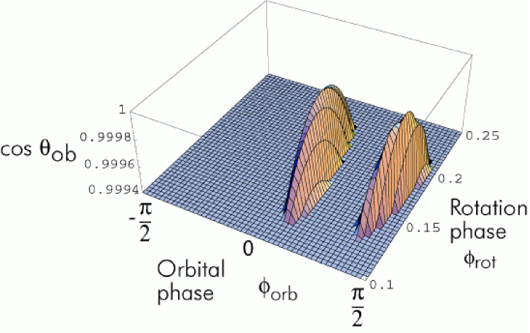
Figure 2: Cosine of the angle $\theta_{ob}$ between the line of sight and the direction of the polar field line in a distorted magnetosphere as a function of rotational phase $\phi_{rot}=\Omega t$ and orbital phase $-\pi/2<\phi_{orb}<\pi/2$ measured from the superior conjunction. Parameters of the model are $\theta_{\Omega}=60^{\circ}$, $\phi_{\Omega}=67.5^{\circ}$, $\chi=73.6^{\circ}$, $C=0.7$. Emission is visible if $\theta_{ob}<2^{\circ}$ corresponding to $\cos\theta_{ob}>.9994$. This happens at two orbital phases $\phi_{orb}=0.03...0.43$ ($1.7^{\circ}...24^{\circ}$) and $\phi_{orb}=1.09...1.45$ ($62^{\circ}..83^{\circ}$).

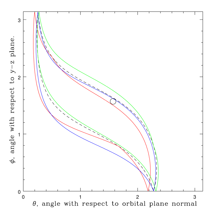
Figure 3: Trajectory of the polar field line on the sky for $\phi_{\Omega}=\pi/8=22.5^{\circ}$, $C=.7$. Black dashed line: undistorted dipole, green solid is at orbital phase $\phi_{orb}=-\pi/4$ (misses the observer), blue line is at orbital phase $\phi_{orb}=0$ and red line is at orbital phase $\phi_{orb}=\pi/4$. The location of observer is denoted by the circle. Upper and lower sets of curves correspond to two magnetic poles.

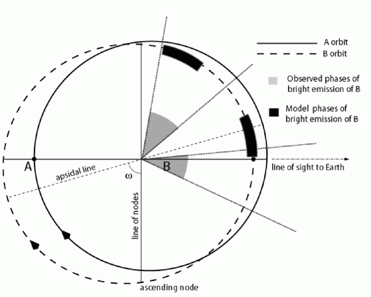
Figure 4: Configuration of the system, after Lyne et al. (2004). Light shades segments indicate orbital phases where B emission is strongest, dark regions indicate the location of emission in the best fit model.

Searching through parameter space we were trying to reproduce two emission windows located in the tail of B magnetosphere. After a number of trials, our best fit parameters are $\phi_{\Omega}=-67.5^{\circ}$ and $C=0.7$. To illustrate the fit, in Fig. 2 we plot a value of $\cos\theta_{ob}={\bf s}_{p}\cdot\hat{\bf x}$ as a function of orbital phase $\phi_{orb}$ and rotational phase $\phi_{rot}$. Only points located above the line $\cos 2^{\circ}=.9994$ produce a pulse of radio emission. (We restrict ourselves to $-\pi/2<\phi_{orb}<\pi/2$, corresponding to the tail pointing towards the observer.) Clearly, in the tail of magnetosphere the polar field lines are pointing toward an observer at two orbital phases separated by approximately $70^{\circ}$, see Fig. 4. One of the phases, nearly coincident with the conjunction, is located at orbital phase $\phi_{orb}=1.7^{\circ}...24^{\circ}$ and the second is located at $\phi_{orb}=62^{\circ}...83^{\circ}$. Considering the simplicity of the model and the fact that we had to make a multi-parameter fit, the agreement with observations is impressive. In order to illustrate the effect of field distortion, in Fig. 3 we plot a trajectory of magnetic polar lines on the sky, folded over $\pi$ radians to show both poles. Emission is seen only at points approaching the direction to the observer within two degrees.

Though we were able to obtains a satisfactory fit, we cannot guarantee that there is no other island in the phase space of 6 parameters that also satisfies these criteria. In addition, there are intrinsic ambiguities in the model, related to prograde versus retrograde rotation of pulsar B and to which magnetic pole is seen by the observer.

5 Discussions and Predictions

We have constructed a simple model of orbital variations of pulsar B emission. Small distortions of the inner magnetosphere of B by pulsar A wind change direction of the polar field lines, pushing radiative beam of B towards the line of sight at two orbital phases. The main implication of the model is that B is always intrinsically bright. The model reproduces fairly well absolute orbital location of bright emission windows, their width $\sim 20^{\circ}$ and separation $\sim 70^{\circ}$. It also naturally explains different profiles at two emission windows, since at different orbital phases the line of sight crosses the emission region along different paths.

In this paper we considered only the nightside magnetosphere. The stretching method does not produce a realistic structure of the dayside (Stern, 1994). Qualitatively, we expect that on the dayside polar field lines will also be shifted from the direction of the magnetic pole and will be pushed out of the line of sight, producing a dip in the light curve of B close to the inferior conjunction. Since emission beam is very narrow and distortions can be considerable, it is fairly easy for the beam of B to miss an observer. A more detailed model of magnetosphere is deferred to a subsequent paper.

Our suggestion that pulsar B is always intrinsically bright is consistent with its spin-down and radio energetics. First, assuming that an extension of the last open field line is determined by the size of magnetosphere and that typical current density flowing on the open field lines is of the order of the Goldreich-Julian current density, the total potential over open field lines (a quantity that is usually related to efficiency of pair production, (e.g.  Arons & Scharlemann, 1979)) is independent of $R_{m}$: $\Phi_{tot}\sim\sqrt{L_{SD}/4\pi c}$, where $L_{SD}=1.6\times 10^{30}$ erg/s is the spindown luminosity of B Lyne et al. (2004). This ranks it as the 20th smallest (but not exceptional) out of nearly 1500 pulsars with measured spindown luminosities (see www.atnf.csiro.au/research/pulsar/psrcat). Secondly, its peak luminosity of $\sim 3$ mJy at 820MHz (Ransom, priv. comm.) is typical for isolated pulsars with similar properties.

There is a number of predictions of the model. First, at different orbital phases the center pulse corresponds to somewhat different rotational phases. Near $\phi_{orb}=1.7^{\circ}$, the center pulse is at $\phi_{rot}\sim 11.5^{\circ}$, decreasing to $\phi_{rot}\sim 8^{\circ}$ at $\phi_{orb}=24^{\circ}$, remaining the same at $\phi_{orb}=62.5^{\circ}$ and increasing back to $\phi_{rot}\sim 11.5^{\circ}$ at $\phi_{orb}=83.1^{\circ}$, see Fig. 5. Thus, one expects a drift of the profile as a function of an orbital phase. Particular values for the drift angle and rate are strongly dependent on the precise parameters of the model, but the type of evolution is generic: during a visible phase the profile drifts approximately by its width. If averaged over a bright emission window, the drift of the emission phase may be interpreted as a large timing noise of B.

A drift of the emission phase as a function of orbital position may have already been observed. Ransom et al. (2004a) reported a systematic change in arrival times of B pulses by 10-20 ms. This is consistent with the prediction of the model, since a change in arrive phase by 2 degrees of rotation phase of B corresponds to $\sim 15$ ms.

In our model, the weak emission of B observed throughout the orbit has a different origin than the bright emission. For example, it can be generated in a much wider cone, akin to interpulse emission (bridges) observed in regular pulsars.

Our second prediction is related to a secular evolution of pulsar B emission properties. The emission beam of B is fairly narrow, so that small changes in the orientation of rotation axis of B may induce large apparent changes in the profile. One possibility for the change in the direction of the spin is a geodetic precession of B, which should happen on a relatively short time scale $\sim 70$ yrs (Lyne et al., 2004). The geodetic precession will affect mostly the angle $\phi_{\Omega}$. From our modeling we find that changes of $\phi_{\Omega}$ by as little as $\sim 1^{\circ}$ strongly affect observed B profile (see Fig. 5). Thus, we expect that profile of B may change on a times scale of less than a year. According to the model, average profile width remains approximately constant. Changes of the orbital phases of emission are not accompanied by substantial changes in the emission phase. (Note that if the emission geometry is non-trivial, e.g. elliptic instead of circular, one does expect changes in the emission phase.) Since at different epochs line of sight passes through different emission regions one may expect variations in pulse intensity. Thus, using different slices taken at different epochs one can construct a detailed map of the emission region. This should prove a valuable method in constraining pulsar radio emission mechanisms.

A longer evolution of the profile cannot be predicted unambiguously since we do not know the direction of the drift. Two possibilities include increasing or decreasing $|\phi_{\Omega}+90^{\circ}|$, see Fig. 6. In one case, two emission regions get closer together merging in one, while in the other case they separate and a new one appears approximately at a mirror reflection of the first, at $\phi_{orb}\sim-90^{\circ}$. We would like to stress again that exact details of the secular evolution are hard to predict using this very simple model.

For the stretching coefficient $C=0.7$, the relative deformation of the magnetosphere at the emission radius is $\sim 30\%$. This is a fairly large distortion, which favors large emission altitudes, $R_{em}\geq 10^{8}$ cm. Large emission altitudes in isolated pulsars have been previously suggested by Lyutikov et al. (1998). A more precise modeling of B magnetic field may reduce required distortion and thus allow somewhat smaller $R_{em}$. Still, near stellar surface distortions are expected to be tiny, so that the model requires high emission altitude.

The success of this simple model is somewhat surprising, given the fact that in all we had to fit many parameters with a required precision of $2$ degrees. Qualitatively, the reason for the success of this model, as well as that of Lyutikov & Thompson (2005), is that, to the first order, magnetic field is well approximated by dipolar structure. Given the simplicity of the model, some of the parameters may not be well determined: small variations in parameters may induce relatively large observed changes.

A number of effects may complicate the picture. First of all, a non-trivial geometry of the emission region, e.g. elliptical instead of circular, may increase the quality of the fit. The fact that B profiles in the two emission windows are different implies that emission geometry is indeed non-circular. A double hump profile in one of the windows also points to a more complicated emission geometry. Secondly, non-spherical A wind will produce distortions dependent on orbital phase. Also, if reconnection between wind and magnetospheric field lines is important, the structure of magnetosphere may depend on the direction of the wind magnetic field . We plan to address these issues in a subsequent paper. Clearly, a detailed modeling of B magnetosphere is required to further finesse the model.

When the paper has been mostly completed we learned the results of Burgay et al.  (2005), who found secular changes in B profiles in general agreement with predictions of the model.

Figure 1: Geometry of the model. Observer is located at $x\rightarrow\infty$. The spin axis of pulsar B is defined by angles $\theta_{\Omega}$ and $\phi_{\Omega}$. The direction of the magnetic moment $\vec{\mu}$ makes angle $\chi$ with the spin axis and rotates around $\Omega$ every 2.77 s. A line connecting two pulsars lies in the x-y plane and makes angle $\phi_{orb}$ with $x$ axis. (Note that we define orbital phase with respect to the point of superior conjunction and not with respect to ascending node. Two definitions differ by $270^{\circ}$.) Tail coordinates $x^{\prime},y^{\prime},z^{\prime}$ are also shown with vector ${\vec{\mu}}$ in the $x^{\prime}-z^{\prime}$ plane. Angle $\theta_{\mu}$ is between $z^{\prime}$ and ${\vec{\mu}}$.

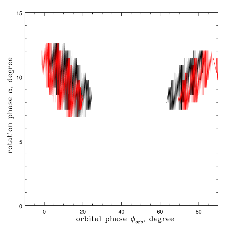
Figure 5: Dependence of the rotation phase of emission on the orbital position and evolution of the emission pattern due to changes of $\phi_{\Omega}$. B radio emission is seen at Earth at two shaded areas. At different orbital phases peak of emission occurs at different rotation phases. Typical variations in emission phase are of the order of the profile width. The corresponding drift of arrival times for pulsar B is $\sim 15$ ms. Region in black is the current best fit $\phi_{\Omega}=-67.5^{\circ}$, region on red is for $\phi_{\Omega}=-68.5^{\circ}$.

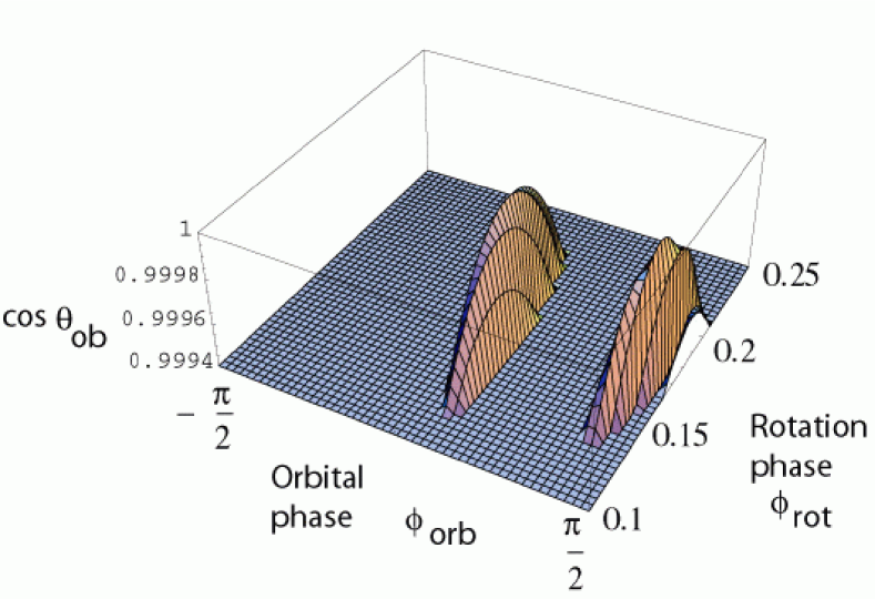
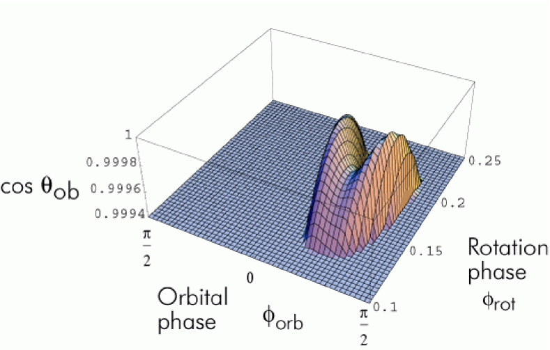
Figure 6: Secular changes in the position of the emission regions due to geodetic drift: (a) $\phi_{\Omega}=-68.5^{\circ}$, (b) $\phi_{\Omega}=-65^{\circ}$ (current best fit value is $\phi_{\Omega}=-67.5^{\circ}$). In case (a) the orbital separation between the two bright phases increases, in case (b) it decreases, so that two phases merge in one. Except for $\phi_{\Omega}$, parameters are the same as in Fig. 2.

References

- Arons et al. (2004) Arons, J., Backer, D. C., Spitkovsky, A., & Kaspi, V. M. 2004, astro-ph/0404159
- Arons & Scharlemann (1979) Arons, J., Scharlemann, E. T., 1979, ApJ, 231, 854
- Burgay et al. (2003) Burgay, M., D’Amico, N., Possenti, A., et al. 2003, Nature, 426, 531
- Burgay et al. (2005) Burgay, M., et al. ,
- Chapman & Ferraro (1930) Chapman, S., Ferraro, V.C.A., 1930, Nature, 16. 129
- Cole et al. (2004) Coles, W. A., McLaughlin, M. A., Rickett, B. J., Lyne, A. G., & Bhat, N. D. R. 2004, astro-ph/0409204
- Demorest et al. (2004) Demorest, P., Ramachandran, R., Backer, D. C., Ransom, S. M., Kaspi, V., Arons, J., Spitkovsky, A. 2004, ApJ, 615, 137
- Goldreich & Julian (1969) Goldreich, P. & Julian, W. H., 1969, ApJ, 157, 869
- Kaspi et al. (2004) Kaspi, V. M., Ransom, S. M., Backer, D. C., Ramachandran, R., Demorest, P., Arons, J., & Spitkovskty, A. 2004, ApJ, 613, 137
- Jenet & Ransom (2004) Jenet, A. F. & Ransom, S. M. 2004, Nature, 428, 919
- Lyne et al. (2004) Lyne, A. G., et al. 2004, Science, 303, 1153
- Lyutikov (2004) Lyutikov, M., 2004, MNRAS, 353, 1095
- Lyutikov & Thompson (2005) Lyutikov, M., Thompson, C., submitted to ApJ, astro-ph/0502333
- Lyutikov et al. (1998) Lyutikov, M., Blandford, R. D., Machabeli, G., 1999, MNRAS, 305, 338
- Manchesteret al. (2005) Manchester, R.N., et al. , 2005, astro-ph/0501665
- Ransom et al. (2004a) Ransom, S. M., Demorest, P., Kaspi, V. M., Ramachandran, R., Backer, D. C., 2004a, astro-ph/0404341
- Ransom et al. (2004b) Ransom, S. M., Kaspi, V. M., Ramachandran, R., Demorest, P., Backer, D. C., Pfahl, E. D., Ghigo, F. D., & Kaplan, D. L., 2004b, ApJ, 609, 71
- Stern (1987) Stern, D., 1987, Reviews of Geophysics, 25, 523
- Stern (1994) Stern, D., 1994, J. Geophys. Res., 99, 2443
- Tsyganenko (1990) Tsyganenko, N. A., 1990, Space Science Reviews, 54, 75
- Zhang & Loeb (2004) Zhang, B., Loeb, A., 2004, ApJ, 614, 53
- Voigt (1981) Voigt, G., 1981, Planet. Space Sci., 29, 1