Variability of Fe II Emission Features in the Seyfert 1 Galaxy NGC 5548

Abstract

We study the low-contrast Fe ii emission blends in the ultraviolet (1250–2200 Å) and optical (4000–6000 Å) spectra of the Seyfert 1 galaxy NGC 5548 and show that these features vary in flux and that these variations are correlated with those of the optical continuum. The amplitude of variability of the optical Fe ii emission is 50% – 75% that of H$\beta$ and the ultraviolet Fe ii emission varies with an even larger amplitude than H$\beta$. However, accurate measurement of the flux in these blends proves to be very difficult even using excellent Fe ii templates to fit the spectra. We are able to constrain only weakly the optical Fe ii emission-line response timescale to a value less than several weeks; this upper limit exceeds all the reliably measured emission-line lags in this source so it is not particularly meaningful. Nevertheless, the fact that the optical Fe ii and continuum flux variations are correlated indicates that line fluorescence in a photoionized plasma, rather than collisional excitation, is responsible for the Fe ii emission. The iron emission templates are available upon request.

1 INTRODUCTION

Emission from singly ionized iron is one of the principal coolants of the broad-line region (BLR) in active galactic nuclei (AGNs): indeed, the prominent blend of Fe ii and Balmer continuum emission in the near UV spectrum, a feature often referred to as the “small blue bump,” produces as much as one third of the line flux in some objects (Wills, Netzer, & Wills 1985; Maoz et al. 1993). Remarkably, however, the characteristics of Fe ii emission in AGNs are very poorly understood from both theoretical and observational perspectives:

1. The excitation mechanism that produces Fe II emission in AGN spectra is not known. Theoretical models, based on either photoionization or collisional excitation, have for a long time fallen short in reproducing the observed Fe ii emission (e.g., Collin & Joly 2000; Baldwin et al. 2004). Also, conflicting results appear in the literature as to the importance of the hard X-rays as an excitation agent as originally anticipated by Davidson & Netzer (1979) and as to that of the slope of the soft X-ray spectrum (e.g., Wilkes, Elvis, & M^cHardy 1987; Shastri et al. 1994; Boroson 1989; Zheng & O’Brien 1990; see also Wilkes et al. 1999). Even with much-improved current models, either significant microturbulence (or velocity shear) in a photoionized medium or a contribution from a collisionally ionized gas seems to be required to account for the strength and shape of Fe ii emission in AGN spectra (e.g., Baldwin et al. 2004). The conditions that are necessary to reproduce the observed Fe ii spectra do not provide clear and straightforward diagnostics to distinguish between these possibilities.

2. Strong, broad Fe II emission pervades the UV through IR spectra of AGNs, contaminating other spectral features. The complex atomic structure of Fe⁺ results in tens of thousands of transitions (e.g., Verner et al. 1999; Sigut & Pradhan 2003) that produce blended features across the UV, optical, and IR spectrum. Isolating individual emission lines under these circumstances is challenging, leading to systematic uncertainties in measurement of emission-line fluxes, widths, and profiles. The intrinsically large line widths of AGN emission lines add to the complexity of this issue.

Further underscoring the importance of understanding AGN Fe ii emission is the possibility of using AGN spectra to measure the cosmic evolution of the abundance of iron, thus providing potentially strong constraints on the history of chemical enrichment due to star formation (e.g., Hamann & Ferland 1999; Dietrich et al. 2003 and references therein, but see also Verner et al. 2004; Baldwin et al. 2004).

A potentially powerful way of exploring the Fe ii emitting region in AGNs is through flux variability, specifically by emission-line reverberation mapping (Blandford & McKee 1982; Peterson 1993, 2001). At minimum, reverberation mapping can be expected to yield the typical distance of the Fe ii-emitting gas from the central continuum source through measurement of the time-delayed response of the emission lines to continuum variations. This would allow us to constrain observationally some of the physical conditions conducive to strong Fe ii emission. For example, variability time scales for the optical and UV Fe ii emission, respectively, will help discern whether or not the multiplets at these energies originate in a common region. This is a key issue for understanding their relative intensity ratio in terms of current Fe ii models which fail to reproduce observations (Baldwin et al. 2004). At the present time, studies of Fe ii flux variability have been very limited:

1. Maoz et al. (1993) used UV data obtained with the International Ultraviolet Explorer (IUE) and optical data obtained with multiple ground-based telescopes by the International AGN Watch over an 8-month period in 1989 to study the variability of the small blue bump in NGC 5548. They concluded that the small blue bump emission arises approximately at the same distance as the Ly$\alpha$ emission, about 10 light days from the continuum source. While in many ways, this represents the best study to date on variability of the small blue bump, it must be noted that (a) the quality of IUE data in this part of the spectrum (i.e., obtained with the LWP camera) is quite poor and (b) there are relatively few epochs in which there is no gap in wavelength coverage between the UV and optical spectra, making measurements of the small blue bump variability systematically somewhat uncertain.

2. Goad et al. (1999) observed the small blue bump in NGC 3516 on six occasions over an 11-month period in 1995–96. Remarkably, while the continuum and high-ionization emission lines varied in flux by a factor of 2, the Mg ii $\lambda 2800$ and Fe ii UV emission did not vary by more than 7% over this time.

3. Kollatschny, Bischoff, & Dietrich (2000) carried out a 20-year study of emission-line variations in NGC 7603 and found that the optical Fe ii blends vary with an amplitude comparable to that of the Balmer lines.

4. Kollatschny & Welsh (2001) searched for and found no optical Fe ii variability in Mrk 110 to within their sensitivity of 10%, although clear optical Fe ii variability is seen in the case of Fairall 9 with an amplitude half that of H$\beta$ (Kollatschny & Fricke 1985).

5. Sergeev et al. (1997) attempt to constrain the time delay of the Fe ii multiplets in the wings of [O iii] $\lambda$5007 in the spectrum of NGC 5548. They find a time delay of a few hundred days. There are, however, a number of serious difficulties with this result arising from strong blending of lines, data quality, and time-series problems.

6. A few other studies make claims of Fe ii variability (Kollatschny et al. 1981; Salamanca, Alloin, & Pelat 1995; Doroshenko et al. 1999). On the basis of spectra of narrow-line Seyfert 1 (NLS1) galaxies taken a year apart, Giannuzzo & Stirpe (1996) find that the optical Fe ii does seem to vary in these sources. For the three sources with detected variability in both H$\beta$ and Fe ii, the Fe ii/H$\beta$ flux ratio ranged from 0.25 to 1.0; this would put Fe ii variability below the detection threshold for the sources in which it was not detected.

Given the importance of understanding Fe ii emission in AGNs and given the limited attention this topic has received in the past, we have undertaken an examination of Fe ii variability in NGC 5548. In terms of emission-line variability, NGC 5548 is by far the best-studied AGN (see Peterson et al. 2002 and references therein). On the other hand, as Baldwin et al. (2004) point out, Fe ii emission is not especially strong in this source and other sources may be better suited to such a study. While we agree with this statement, we also feel that the wealth of data on other lines in NGC 5548 affords a special context in which to examine Fe ii variability and, of course, suitable data for this study already exist. Moreover, cursory consideration of Fe ii variability in NGC 5548 yields mixed impressions. For example, the difference between spectra taken at recent historical maximum and minimum flux states (see Peterson et al. 1999, Figure 3) seems to clearly show optical Fe ii emission, indicating that these blends do indeed vary in this source. However, Kollatschny & Welsh (2001) attribute the apparent variations solely to changes in He ii $\lambda 4686$. If indeed the optical Fe ii emission varies with time, then we ought to see evidence of these features in the difference or rms spectra (defined below in §2.3.2.) that we use to isolate the variable parts of the emission lines (e.g., Peterson et al. 2004); our initial impression is that the optical Fe ii blends do not appear in rms spectra and thus there is no compelling evidence for optical Fe ii variability, at least on time scales of several months.

Thus, the goal of this study is to determine whether or not Fe ii emission varies in NGC 5548 and, if so, with what amplitude and on what timescale. We also attempt to constrain meaningfully the Fe ii line width as an additional test of the common assumption that the optical Fe ii emission arises co-spatially with the Balmer lines (e.g., Phillips 1978). We will not specifically re-examine the issue of the variability of the small blue bump since the data examined by Maoz et al. (1993) have not been superseded by superior data and we are unlikely to be able to improve on their results. We will thus concentrate on variability of the optical Fe ii features, comprised primarily of two blends, one between H$\gamma$ and H$\beta$, and the other covering the spectral ranges 5100–5700 Å (often referred to as the 4570 Å and 5190, 5320 Å blends, respectively; Osterbrock 1976), and of the UV Fe ii blends in the vicinity of the C iv $\lambda 1549$ emission line.

2 METHODOLOGY AND DATA ANALYSIS

2.1 Data

As noted above, we are focusing on NGC 5548 on account of the large amount of variability data available. There are two suitable UV data sets. The first of these is a set of IUE spectra obtained over an 8-month period in 1988–89, sampled once every four days (Clavel et al. 1991). The second set of UV spectra were obtained with the Faint Object Spectrograph (FOS) on Hubble Space Telescope (HST) over a 39-day period in 1993, sampled once per day (Korista et al. 1995); this second set was supplemented by additional IUE data that we will disregard in this study as they are far less suitable than the HST data for the present purposes. Both UV data sets were recovered from the International AGN Watch website. The IUE spectra used were those processed with the IUE New Spectral Image Processing System (NEWSIPS; Nichols et al. 1993). The HST spectra were processed as described by Korista et al. (1995).

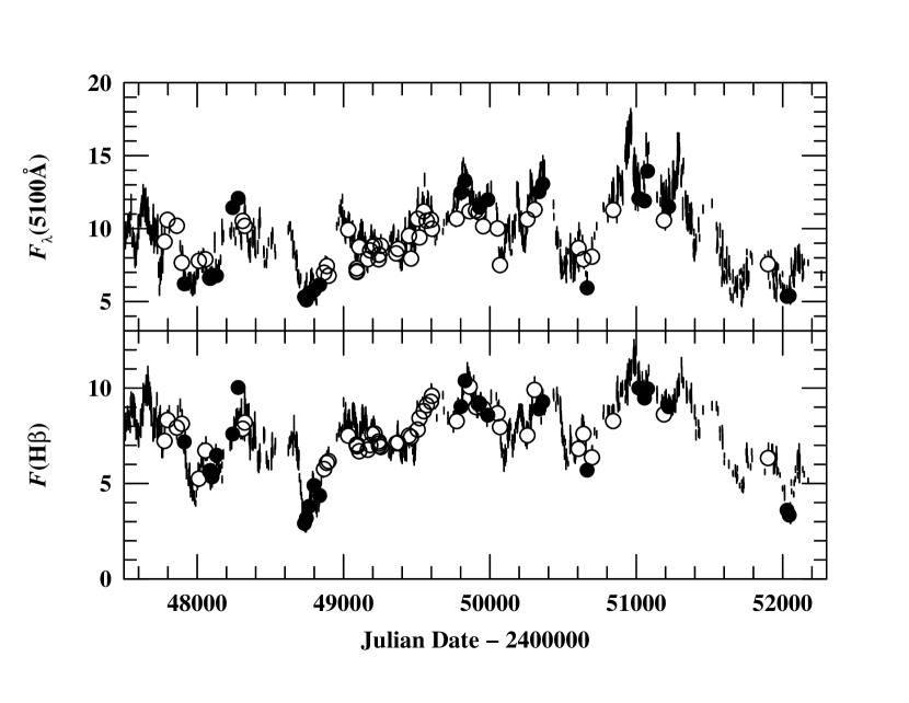
Figure 1: Optical continuum (upper panel) and H$\beta$ (lower panel) light curves for NGC 5548 for the period 1988 to 2001. The vertical lines show the $\pm 1\sigma$ error ranges for the light curves based on the International AGN Watch database (Peterson et al. 2002 and references therein), and the open and filled circles show the measurements based on the 73 rescaled spectra used in this study. The filled circles mark the epochs of the data used to construct the low and high state spectra shown in Figure 4 and described in section 2.3.1. Continuum fluxes are in units of $10^{-15}$ ergs s^-1 cm^-2 Å^-1, and H$\beta$ fluxes are in units of $10^{-13}$ ergs s^-1 cm^-2. The distribution of open and filled circles shows that this particular subset of spectra represents the entire database very well.

In addition to the UV spectra, there are 1248 optical spectra that were obtained beginning in 1988 (i.e., concurrently with the IUE spectra described above) for 13 years through 2001 (Peterson et al. 2002 and references therein). However, only a relatively small subset of these data are suitable for studying variability of the optical Fe ii blends; the Fe ii blends are broad, low-contrast features that can be measured or modeled usefully only in high-quality spectra. Also, as discussed below, we find that Fe ii variability is most reliably measured by combining spectra to form difference spectra (i.e., subtraction of a low flux state spectrum from a high flux state spectrum) or rms spectra in order to isolate the parts of the spectrum that are varying. Since the amplitude of variability is small and since combining spectra propagates noise, it is essential to start out with high-quality data. Specifically, we require high signal-to-noise ratios, reasonably high spectral resolution in order to detect structure in the Fe ii blends, and high-fidelity relative flux calibration over an extended wavelength range in order to constrain the underlying continuum level. Moreover, the necessity of combining spectra requires that we select a homogeneous subset of the data. Given these requirements, the best subset is drawn from those obtained with the Lick Observatory 3-m telescope by A.V. Filippenko and collaborators (“Set H” described by Peterson et al. 2002 and references therein). We selected from this subset all high-quality spectra that cover the observed wavelength range 4000–6000 Å. These criteria yielded 73 spectra spanning the entire 13 years of the International AGN Watch program in a fairly representative way. These 73 spectra were put on a common flux scale by assuming that the narrow-line [O iii] $\lambda\lambda 4959$, 5007 fluxes are constant with $F(\mbox{\rm[O\,{\scriptsize III}]})\,\lambda 5007=5.58\times 10^{-13}$ ergs sec^-1cm^-2 (Peterson et al. 1991). This was accomplished using a version of the van Groningen & Wanders (1992) flux scaling algorithm. After scaling each spectrum in flux, we verified the consistency of the calibration by measuring the continuum flux at 5100 Å and the total H$\beta$ flux in each spectrum. Figure 1 shows a comparison of the continuum and H$\beta$ fluxes measured here with published fluxes based on all of the International AGN Watch data. Agreement appears to be excellent. Figure 1 also underscores the point that the spectra we have selected for study are a suitably representative subset of the entire database.

2.2 Fe II Templates

As noted above, the complex atomic structure of Fe⁺ produces a large number of transitions that pervade the UV, optical, and IR spectrum. Doppler broadening within the BLR causes the Fe ii emission lines to blend together and with lines of other species, thus making it extremely difficult to accurately measure the Fe ii emission-line flux. However, it was first noted by Phillips (1977, 1978) that the optical Fe ii spectra of Seyfert 1 galaxies are very similar, differing from one AGN to the next primarily in the amount of Doppler broadening. In this context, the Seyfert 1 galaxy I Zw 1 (Sargent 1968; Phillips 1976) is of particular interest: the widths of the Fe ii and Balmer lines in this source are only $\sim 1100$ km s^-1, among the very narrowest permitted lines observed in Seyfert 1 spectra. Phillips demonstrated that by suitably broadening the I Zw 1 spectrum to match the broad H$\beta$ widths of other Seyfert 1s, the observed Fe ii profiles could be matched reasonably well. This suggested that the Fe ii emission arises co-spatially with the broad H$\beta$ emission. This also suggested to Boroson, Persson, & Oke (1985) and Boroson & Green (1992) that the broadened I Zw 1 spectrum could be used as a template to model the Fe ii contribution to AGN emission-line spectra, although of course their interest was more focused on removing Fe ii as an emission-line contaminant than in using it to determine the Fe ii emission flux. Boroson & Green used high-quality spectra of I Zw 1 to develop an Fe ii emission-line template that could be used generally to remove Fe ii emission from AGN spectra over the range 4250–7000 Å. Recently, a revised and improved optical Fe ii template based on I Zw 1 and covering the range 3535–7534 Å has been prepared by Véron-Cetty, Joly, & Véron (2004). It is this template, shown in Fig. 2, that we use in analysis of the optical spectra of NGC 5548. Templates with a range of intrinsic line widths were generated by folding the entries of Fe ii transitions listed in Table A.1 of Véron-Cetty et al. (their broad system L1) with Lorentzian profiles of different FWHM.

A similar template for the UV spectrum (1250–3090 Å), again based on I Zw 1, has been constructed from HST spectra by Vestergaard & Wilkes (2001). We use this template, shown in Fig. 3, to attempt to model the UV Fe ii emission in NGC 5548. Vestergaard & Wilkes present several versions of UV iron templates, including separate templates of Fe ii and Fe iii emission, respectively, each of which have options of including or excluding certain multiplets that are characteristically strong in I Zw 1. Two templates of UV iron emission were fit to the NGC 5548 data: (1) a template consisting only of Fe ii emission transitions, excluding Fe ii UV 191 at 1786 Å, and (2) a template consisting of both Fe ii and Fe iii emission transitions, excluding Fe ii UV 191 and Fe iii UV 34 as these multiplets are particularly strong in I Zw 1 and the spectra of NGC 5548 show little indication of their presence. As will be clear from § 2.4, the template that includes Fe iii emission provides a poor fit to the data. We note that the Fe ii emission shortward of the C iv emission line tends to be overpredicted by using the template as originally presented by Vestergaard & Wilkes. Forster et al. (2001) came to a similar conclusion for a small fraction of the spectra in their sample. The bluest part of the HST spectrum of I Zw 1 (below $\sim$1500 Å) on which the UV template is based was not observed at the same time as the longer-wavelength segments and I Zw 1 increased in luminosity between these two observations. Vestergaard & Wilkes rescaled the shortest-wavelength segment to match the longer-wavelength part of the spectrum to produce a full-range UV template. However, it was recognized then that the Fe ii emission in the template below $\sim$1550 Å may need to be rescaled for some objects. By fitting the NGC 5548 spectra we found that very reasonable fits can be obtained by applying a scaling factor of 0.25 to the template Fe ii emission shortward of 1550 Å.

The general fitting procedure used here is described by Vestergaard & Wilkes (2001; section 4.2 in that paper). A power-law continuum is subtracted from the spectrum, which makes the Fe ii emission more visible, before fitting the Fe ii templates. The power-law continuum is fitted to windows that are virtually free of line emission, namely $\sim$4200 Å and $\sim$5650 Å in the optical and $\sim$1350 Å and $\sim$2000 Å in the UV. An iteration over continuum setting and Fe ii template fitting may be necessary to get the best fit. We consider the best template fit to be that which leave the residual spectra virtually featureless in regions dominated by Fe ii. Additional details on our fitting of the optical spectrum of NGC 5548 are given in §2.3.3.

2.3 Optical Fe II Blends

We made an initial attempt to fit each of the 73 selected spectra with the optical Fe ii template. We found this to be very difficult because of blending of Fe ii with other features in the spectra, notably weak narrow lines and small-scale structure due to features in the underlying galaxy spectrum. Given the problems we encountered, we had little confidence in these results.

2.3.1 Difference Spectra

We therefore began experimenting with alternative approaches that would mitigate some of the problems due to contaminating features. One method is to produce difference spectra, i.e., to subtract a low flux-state spectrum from a high flux-state spectrum. This effectively removes all the non-variable components from the spectrum, including narrow emission lines and host galaxy light, although sometimes small residuals of these features can be seen, usually as a consequence of seeing and aperture effects (e.g., Peterson et al. 1995) or small differences in the line-spread function between pairs of observations. A potential liability of this approach is that the uncertainties in difference spectra can be fairly large; the differences between two spectra are often quite small, but the uncertainties add in quadrature. We attempted to mitigate this problem by making a high signal-to-noise ratio low-flux state spectrum by co-adding a number of individual faint-state spectra, and then subtracting this “standard low-state spectrum” from all of the individual spectra. To form a standard low-state spectrum, we identified several spectra obtained during the faintest periods in the 13-year monitoring program. The standard low-state spectrum as formed by averaging 3 spectra from the fourth year of the AGN Watch program (specifically, the spectra obtained on Julian dates 2448733, 2448765, and 2448810) with two spectra obtained during the thirteenth year (on Julian dates 2452030 and 2452045).

Use of difference spectra greatly improved our ability to model the optical Fe ii emission with a template, although the results were still not quite satisfactory. We found that there was degeneracy at about the 10% level in fitting the Fe ii fluxes (i.e., changes in flux of 10% made no discernible difference in the overall quality of the fit). Moreover, comparison of the inferred Fe ii fluxes between observations that are closely spaced in time often showed large differences; indeed, if the errors are random, we would infer that the level of precision of the Fe ii fluxes is only $\sim 30$%, about an order of magnitude more uncertain than our H$\beta$ fluxes (cf. Peterson et al. 2002). Despite these large uncertainties in individual spectra, we nevertheless find a clear correlation between the continuum flux at 5100 Å and the Fe ii flux. We find a Pearson’s linear correlation coefficient of 0.73 and a probability of a chance (or null) correlation below 0.0001. While we caution about placing too much emphasis on the specific numbers, these results emphasize the reality of such a correlation.

These measurements establish that the optical Fe ii fluxes do indeed vary in a way that is correlated with the continuum. However, we are unable to establish a timescale for the response of the optical Fe ii blends to continuum changes, i.e., to measure a reverberation lag. First, the sampling of these 73 spectra is comparatively sparse, as can be seen clearly in Fig. 1. The median interval between observations is nearly 60 days. For reference, cross-correlation of the 73 optical continuum and H$\beta$ fluxes measured from these spectra and displayed in Fig. 1 yield time delays $\tau_{\rm cent}=5.3\pm 11.8$ days and $\tau_{\rm peak}=17\pm 4$ days, where these two quantities are respectively the centroid and peak of the optical continuum/H$\beta$ cross-correlation function; both of these measurements are consistent with the result obtained using all the AGN Watch data shown in Fig. 1, although the centroid value is formally highly uncertain. Second, the very large uncertainties in the optical Fe ii fluxes obviate any chance of obtaining even a marginal time-lag measurement. Formally, cross-correlation of the continuum and Fe ii light curves yields $\tau_{\rm cent}=12\pm 27$ days and $\tau_{\rm peak}=11\pm 34$ days with a peak correlation coefficient $r_{\rm max}=0.75$. We can conclude, however, that the lag for the optical Fe ii emission is less than several weeks; this is not an especially stringent upper limit as it exceeds the value of any other reliably measured lag in NGC 5548.

Our original planned strategy had been to start with the most suitable optical spectra and progress to the less suitable, but better time-sampled data. However, we abandoned that approach when these initial results made it clear that measuring the Fe ii fluxes accurately even in the best data is extremely difficult; measuring the Fe ii fluxes in less suitable data would not improve the situation.

Inspection of the fits to our 73 difference spectra indicate that the difficulties in accurately fitting Fe ii templates to the spectra are largely attributable to noise in the spectra, of both Poisson and non-Poisson origin. In other words, we might hope to obtain more accurate flux measurements by combining not only low-state, but high-state spectra as well. This proved to be essential for estimating the amplitude of Fe ii flux variability. In this case, we examined the continuum flux measurements for all the AGN Watch data in Fig. 1 and computed their mean and standard deviation. We defined a mean high-state spectrum by combining all of the spectra in our selected sample of 73 spectra for which the continuum flux is more than one standard deviation above the mean value. These spectra are those obtained on Julian dates 2448243, 2448280, 2449802, 2449830, 2449930, 2449986, 2450336, 2450361, 2451017, 2451056, 2451077, and 2451221. Similarly, we defined a mean low state spectrum by combining all of the spectra for which the continuum flux is more than one standard deviation below the mean values; the spectra that meet this criterion were obtained on Julian days 2447912, 2448089, 2448102, 2448132, 2448733, 2448746, 2448765, 2448798, 2448837, 2450664, 2452030, and 2452045. We then computed the difference between these two in order to produce a high signal-to-noise ratio difference spectrum, as shown in Figs. 4 and 5.

2.3.2 Mean and RMS Spectra

Another approach to more clearly isolating the variable part of the spectrum (and thus suppressing the constant components that contaminate the optical Fe ii spectrum) is to compute a root-mean-square (rms) spectrum. Using all of the 73 spectra in the sample, we formed a mean spectrum,

$$\overline{F(\lambda)}=\frac{1}{N}\sum_{i=1}^{N}F_{i}(\lambda),$$ (1)

where $F_{i}(\lambda)$ is the $i$th spectrum of the $N$ spectra that comprise the database. Similarly, the rms spectrum is defined by

$$S(\lambda)=\left[\frac{1}{N-1}\sum_{i=1}^{N}\left(F_{i}(\lambda)-\overline{F(\lambda)}\right)^{2}\right]^{1/2}.$$ (2)

The mean and rms spectra formed from our 73 optical spectra are shown in Fig. 6. This mean spectrum is the only spectrum which we fitted for this discussion that does not strictly contain variable emission components only. The mean spectrum was fitted to allow assessment of the relative Fe ii variability amplitude.

2.3.3 Identifying the Best Fitting Method of the Optical Iron Emission in NGC 5548

The 4450–4650 Å and 5050–5600 Å regions of AGN and quasars are commonly dominated by Fe ii emission which can be reasonably well-fitted by an optical Fe ii template generated from the I Zw 1 emission spectrum (Boroson & Green 1992; Véron-Cetty et al. 2004). However, we were unable to fit these regions in the NGC 5548 optical spectra with either the Véron-Cetty et al. or the Boroson & Green templates in their original form, i.e., with relative line intensities as observed in I Zw 1. The top panel of Fig. 7 illustrates the result of accounting for all the flux at $\sim 4500$ Å above a power-law continuum with the Véron-Cetty et al. Fe ii template. Clearly, this strongly overpredicts the Fe ii flux in the 5050–5700 Å range. Fitting the template to match the 5050 – 5600 Å Fe ii features instead leaves strong residuals at $\sim 4500$ Å.

We examined three possible solutions to this problem. First, the Fe ii features may not have the relative line intensity as observed for I Zw 1. Second, the emission at $\sim$4500 Å may be due to extended wings of some combination of H$\gamma$, He ii $\lambda 4686$, and H$\beta$. Third, additional line emission, previously unaccounted for, may be present. We address each in turn in the following.

1. We did indeed find that the spectra could be fitted well if the 5050–5600 Å Fe ii features in the template are rescaled. The best fits to the mean, difference, and rms spectra of such modified Véron-Cetty et al. (or Boroson & Green) templates yields scalings relative to (fixed) $\sim$4500 Å Fe ii strength of $\sim$0.4, 0.25, 0.2, respectively. However, such low intensity ratios are not commonly seen in AGN spectra; relative intensities of 0.7 – 0.8 seem more typical. Also, it is apparently difficult to obtain very low intensity ratios of these lines in standard photoionization equilibrium modeling (M. Joly 2004, private communication). This solution is hence not particularly attractive.

2. To test if extended wings of the H$\gamma$, He ii, and H$\beta$ lines can account for the $\sim 4500$ Å residual emission seen in the lower panel of Fig. 7 we fitted Gaussian functions to H$\gamma$ and He ii $\lambda 4686$, while a combination of Gaussian and Lorentzian functions was necessary to reproduce the (variable) H$\beta$ profile. These modeled lines were then subtracted from the data. The results are shown in Fig. 8. The upper panel shows the best-fit width to the He ii line of 10,000 km s^-1(FWHM). A strong residual feature at 4500 Å shows that we still cannot account for all the flux in this region. A second attempt with a broader (12,000 km s^-1 FWHM) He ii line, as shown in the lower panel of Fig. 8, results in very little improvement.

3. An alternative explanation is that additional previously unidentified line emission is present in the NGC 5548 spectrum. Although emission lines other than Fe ii are rarely seen at $\sim 4500$ Å in quasars (e.g., Boroson & Green 1992), NGC 5548 may have a strong contribution of He i $\lambda$4471, given the presence of strong He i $\lambda$5876 observed at the edge of the spectra (Figs. 4, 5, and 6). In fact, the presence of He i $\lambda$5876 also implies the existence of the He i singlet lines at 4922 Å and 5016 Å. Common intensity ratios to He i $\lambda$ 5876 are 0.3, 0.1, and 0.1 for the 4471 Å, 4922 Å, and 5016 Å lines, respectively, although the 4471 Å intensity ratio may be as low as 0.1 (K. Korista 2004, private communication). Both panels of Fig. 8 illustrate that the excess emission at $\sim 4500$ Å remaining when subtracting other known sources of line emission is consistent with the presence of He i $\lambda$4471 (thin solid curve) at an intensity of 0.3 times that of He i $\lambda$5876.

These arguments collectively justify our inclusion in our general fitting of the non-apparent He i $\lambda\lambda$4471, 4922, 5016 lines with the above-mentioned intensity ratios as found in photoionization equilibrium modeling. Figure 5 illustrates the method we thereafter adopted for fitting the Fe ii emission: the expected He i features, based on the observed 5876 Å line, were subtracted before fitting the Fe ii emission. The adopted template fitting of the difference, mean, and rms spectra are shown in Figs. 4 and 6.

We note that both the broad He i $\lambda$5876 and He ii $\lambda$4686 features are observed shifted to the blue by $\sim$1000 km s^-1 to 1500 km s^-1; this is apparent even in the observed spectra. It is particularly clear in the mean spectrum (Fig. 6) where the narrow He i $\lambda$5876 component is observed at 5876 Å yet the peak of the broad component is blueshifted; we reproduced this shift when modeling and subtracting the expected He i lines in the mean spectrum. Interestingly, there is no clear indication that the (broad) He ii $\lambda$1640 line is shifted by such a large amount.

Upon subtraction of the best-fit Fe ii templates, a few small residuals may still remain, especially in the mean spectrum (Fig. 6) where some non-variable possibly narrower Fe ii transitions may be present; we did not attempt to include any transitions of the narrower Fe ii system identified by Véron-Cetty et al. (2004), on the assumption that these would not appear in our difference or rms spectra, which appears justified by Figs. 4 – 6. It is noteworthy that many of the smaller-scale features seen atop the 4450–4750 Å emission blend in the mean spectrum are consistent with the expected positions of Fe ii m38.

2.3.4 Results

Our analysis of the optical Fe ii data on NGC 5548 leads us to the conclusion that the Fe ii emission is indeed variable in flux and that these variations are positively correlated with continuum variations. We are unable, however, to make any meaningful determination of any time delay between the continuum and Fe ii emission blend variations.

In an attempt to assess the amplitude of variability of the optical Fe ii emission, we integrated the Fe ii flux in the best-fit template over the range 4250–5710 Å and divided it by the H$\beta$ broad-line flux as measured in the mean, difference, and rms spectra, respectively. The results are shown in Table 1. Comparison of the Fe ii/H$\beta$ flux ratio in the variable spectra with the mean spectra shows that this ratio is only 25–50% smaller in the variable spectra. This implies that the optical Fe ii emission varies with an amplitude of 50–75% that of the broad H$\beta$ component. The reason that Fe ii emission is not always obvious in rms spectra is simply because the variations are generally rather small, and the low-contrast Fe ii features are weak relative to H$\beta$ and do not show up very well even in high-quality difference or rms spectra.

The best fit we achieve is with an optical Fe ii template broadened to a width similar to that of the variable H$\beta$ line; the H$\beta$ line width in the rms emission-line spectrum shown in the lower panel of Fig. 6 is about 6250 km s^-1. Interestingly, this template gives only a slightly improved fit to the 5050 – 5600 Å Fe ii features relative to templates of somewhat broader widths of $\sim$10,000 km s^-1; the differences in the fit and residuals are practically insignificant.

It is also worth noting, however, that for broadening larger than $\sim 9000$ km s^-1, the templates become essentially degenerate, i.e., it is hard to distinguish among them.

Given that reasonable fits are obtainable with a range of template line widths, we carried out additional tests to try to determine the maximum and minimum line widths for which the template fitting process gives unacceptable results. We find a range of template line widths that yield “acceptable” fits, and a smaller range that are “preferred,” for which even better fits are obtained. The degeneracy is mainly due to the flux density uncertainties in the difference spectra (section 2.3.1) and the relatively minute differences in the detailed shapes of Fe ii templates that differ by 250–750 km s^-1 in line widths, especially for large line widths (above about 6000 km s^-1). For the optical difference and rms spectra, which are not contaminated by non-variable emission, we find that the template fits are unacceptable at line widths less than 4500 km s^-1; “preferred” fits were obtained for widths above 5750 km s^-1, and our “best fit” value of 6250 km s^-1 is a subjective assessment that this provides the best overall fit to the spectrum. Establishing an upper limit on the broadening is more difficult because of the stronger degeneracy of the templates with line widths above about 9000 km s^-1. We are unable to place any meaningful constraints on the upper limit to the Fe ii line widths.

Subtraction of the optical Fe ii template leaves He ii $\lambda 4686$ in the residual spectrum. The width of this line in the residual spectrum is very broad, $\sim 12,000$ km s^-1, and the width is insensitive to which Fe ii template is used, i.e., the difference between using the 6250 km s^-1 and 10,000 km s^-1 templates changes the He ii $\lambda 4686$ width by less than about 200 km s^-1. This He ii $\lambda 4686$ line width is very similar to the width of He ii $\lambda 1640$ measured in the Fe ii subtracted UV difference and rms spectra, discussed below, and to the He ii $\lambda 1640$ width obtained during both UV monitoring campaigns, and significantly larger than the width of He ii $\lambda 4686$ measured in the rms spectrum, with no attempt to account for the possible effects of Fe ii, during the first year of the NGC 5548 monitoring campaign (Peterson et al. 2004). It is not clear, however, whether the He ii $\lambda 4686$ width varies with time, as does, for example, the width of H$\beta$, or if the base of the He ii $\lambda 4686$ line gets broader when the Fe ii is removed. Certainly, the responses of He ii $\lambda 1640$ and He ii $\lambda 4686$ are expected to be identical (Bottorff et al. 2002), and the lags are, in fact, consistent within their uncertainties (Peterson et al. 2004). Indeed, there seems to be no strong evidence that either the lags or line widths of He ii $\lambda 1640$ and He ii $\lambda 4686$ are significantly different from one another. The concerns of Bottorff et al. about the differences in the response of these two lines may be not as significant as previously thought.

2.4 UV Fe II Blends

2.4.1 UV Difference Spectra

In order to determine whether or not the UV Fe ii emission blends vary with the continuum, we carried out an analysis similar to that described above for the optical emission lines, though in this case we describe only our investigation of difference spectra. For both UV data sets described in §2.1, we computed mean high-state and mean low-state spectra, again using the criteria that these spectra have continuum fluxes that are one standard deviation above and below the mean flux, respectively. The HST high state spectrum included those obtained on Julian dates 2449121, 2449122, 2449123, and 2449124, and those that comprise the low-state spectrum are those obtained on 2449097, 2449098, and 2449100. These spectra and their difference are shown in Figs. 9 and 10. For the IUE data, the high-state spectrum was constructed from the spectra obtained on Julian dates 2447538, 2447543, 2447546, 2447621, 2447625, 2447629, 2447633, 2447634, 2447637, 2447638, 2447641, 2447645, and 2447649, and the low-state spectrum is based on the spectra obtained on Julian dates 2447577, 2447581, 2447688, 2447692, 2447729, 2447733, 2447737, 2447741, and 2447745. These spectra and their difference are shown in Figs. 11 and 12.

2.4.2 Results

We fit the difference spectra with two types of template, (1) a pure Fe ii template, and (2) a template that includes both Fe ii and Fe iii. Both templates are from Vestergaard & Wilkes (2001) and described in § 2.2. While Fe ii is clearly present in the difference spectrum, it is not clear that Fe iii is present. If Fe iii is present, it is very weak. We find that inclusion of Fe iii is not necessary to model the spectrum, and the spectrum is better fit by the pure Fe ii template. One possible exception is the bump at $\sim$2200 Å, which is most likely Fe iii (Vestergaard & Wilkes 2001). However, the results of this study are not sensitive to the strength of this feature and we will not consider it any further. Compared to the HST spectrum, the IUE spectrum is harder to fit because it is noisier and covers a shorter wavelength range. On the other hand, if we constrain the slope of the IUE difference spectrum by using the slope measured in the HST difference spectrum, we obtain a satisfactory fit. We find that a better fit is obtained with the 10,000 km s^-1 template than for the 6250 km s^-1 template (Figs. 10 and 12). In particular, we find unacceptable fits using templates with broadenings less than 8250 km s^-1. Given the same issues pertaining to the optical spectra, we are unable to place any upper limits on template broadenings which produce acceptable fits.

We also compare the strengths of the UV Fe ii blends (integrated across the two intervals 1430–1500 Å and 1685–1850 Å) and H$\beta$ in the variable part of the spectrum with what is observed in the mean spectrum, as we did with the optical Fe ii emission above. The results of this comparison are given in Table 2. We see here that the UV Fe ii/H$\beta$ flux ratio is significantly larger in the variable part of the spectrum than in the mean spectrum (we note in passing that analysis of the UV mean and rms spectra leads to the same conclusion). Unlike the optical Fe ii emission, the UV Fe ii emission seems to vary with a larger amplitude than H$\beta$.

3 DISCUSSION

The principal result of this study is that the optical and UV blends of Fe ii emission in the spectrum of NGC 5548 do indeed vary with time. These variations are correlated with the continuum variations. The optical Fe ii blends vary with an amplitude 50–75% that of H$\beta$, and the UV Fe ii blends seem to vary with an even larger amplitude than H$\beta$. The variations of these low-contrast features are most clearly seen in difference or rms spectra, which remove non-variable structure in the spectra. However, the variable Fe ii features are not always obvious in difference or rms spectra simply because these features are often lost in the noise. Previous claims of the lack of variability of Fe ii seem to be consistent with this conclusion, given the sensitivity of the observations. Unfortunately, on account of the weakness of these features in difference or rms spectra, we are unable to determine the time scale for response of the Fe ii emission lines to continuum variations.

We note in passing that very broad Fe ii features produce a “pseudo-continuum” (e.g., Wills et al. 1985) that is not readily identified as line emission. For example, Figs. 9 and 11 (upper panels) show that the 1700–1900 Å region in NGC 5548 is relatively flat, giving the appearance that no (variable) emission lines are present, even though this region is at a somewhat higher level than the continuum at $\sim$1450 Å and 2025 Å. However, the presence of Fe ii emission in this spectral range is clear when fitting the spectrum with an Fe ii template.

Interestingly, we find that the UV Fe ii features in the difference or rms spectra are best fitted with templates that have a large velocity width, $\sim$10,000 km s^-1; the optical Fe ii features are consistent with both such a broad template and one of the variable H$\beta$ line width. We have no ready explanation for this result, although we might speculate that it may be related to the issues responsible for the difficulty of accounting for the strength of the Fe ii (Baldwin et al. 2004), including the unusual smoothness of the Fe ii emission; either microturbulence or velocity shear seems necessary to account for the discrepancy between theory and observation.

The issue of whether or not the optical and UV Fe ii is emitted from the same region is important for theoretical modeling of their relative emission strengths (Baldwin et al. 2004). While the errors on the Fe ii emission-line response time are very large, it is possible to constrain the size of the Fe ii-emitting regions indirectly through the line-broadening parameters under the assumption that Fe ii follows the same virial relationship seen in every other well-characterized variable line in NGC 5548 (Peterson & Wandel 1999). If we assume that the virial product $c\tau_{\rm cent}{\rm FWHM}^{2}/G$ is the same for all lines in NGC 5548, using measurements from Peterson et al. (2004), we can conclude that the optical Fe ii emission, with ${\rm FWHM}>4500$ km s^-1, arises at $r<24$ light days, and the UV Fe ii emission, with ${\rm FWHM}>8500$ km s^-1, arises at $r<7$ light days. This limit on the size of the optical Fe ii emission gas does not violate the weak constraint on the time delay of several weeks based on cross-correlation of the continuum and optical Fe ii emission light curves (section 2.3.1). Given the assumptions, this is a weak conclusion, but it is worth noting that differing line widths for the UV and optical Fe ii emission suggests that the UV and optical Fe ii might be emitted predominantly from different regions within the BLR. If indeed the BLR gas density increases steadily and smoothly toward the center of the BLR, the distance limits are broadly consistent with expectations from photoionization models (e.g., Fig. 11 of Baldwin et al. 2004), namely that UV Fe ii is most efficiently emitted from higher-density gas (presumably located closer to the central source), while optical Fe ii is more efficiently emitted from lower-density gas farther out.

Véron-Cetty, Joly, & Véron (2004) find that the I Zw 1 Fe ii emission spectrum is comprised of two components of different widths, $\sim$1100 km s^-1 and $\sim$300 km s^-1, the latter mostly being forbidden iron transitions. This suggests that some of the Fe ii emission originates in the narrow-line region. The fact that no variations are detected in the narrow Fe ii features by virtue of their absence in the residual spectra of the difference and rms spectra is consistent with this explanation; blends of narrow Fe ii lines may be present in the mean optical spectrum, especially longward of [O iii]. We cannot identify narrow Fe ii in any of the UV spectra we have examined.

Our conclusion that the amplitude of optical Fe ii variability is somewhat smaller than that of H$\beta$, but is often of too low contrast for reliable detection, seems consistent with results for other sources (Kollatschny et al. 1981; Kollatschny & Fricke 1985; Giannuzzo & Stirpe 1996; Doroshenko et al. 1999). Apparent exceptions are Fairall 9 and NGC 7603. Kollatschny et al. (2000) found the optical Fe ii to vary as strongly as H$\beta$ for NGC 7603. In the case of Fairall 9, Kollatschny & Fricke find that both H$\beta$ and the optical Fe ii emission vary with large amplitudes, by factors of 5.6 and 2.6, respectively. For more direct comparison with this result, we restricted our Fe ii measurement window to the 4570Å, 4928 Å, and 5018 Å multiplets, the approximate region used by Kollatschny & Fricke, and found similar values to those we quote in Table 1. We conclude that the relative amplitudes of Fe ii and H$\beta$ flux variability amplitudes can differ significantly among AGNs.

As current photoionization models fall short in reproducing the observed AGN Fe ii emission, Collin & Joly (2000) suggest that Fe ii in AGNs is due entirely to shock (i.e., collisional) excitation. They draw parallels with strong Fe ii emitting stellar sources which have no X-ray or ionizing emission, but do have strong variability and strong outflows. Baldwin et al. (2004) do find that collisional excitation can explain the observed Fe ii, though they are reluctant to consider introduction of another component, which produces no other significant emission, into an already complex picture of the BLR. Moreover, it is not clear how such a model could reproduce the observed correlation between the optical Fe ii and the continuum fluxes that we observe.

The template fits show that the I Zw 1 Fe ii templates are generally reasonably good matches to the optical and UV Fe ii emission from NGC 5548. The exceptions are, as noted earlier, the apparent absence of the Fe iii transitions over the range 1825–2100 Å and the poor match of the original templates at 2025 Å where the Fe ii emission appears to be missing.

4 CONCLUSIONS

Our chief conclusions of our study of the Fe ii emission in NGC 5548 can be summarized as follows:

1. The optical and UV Fe ii emission blends do indeed vary in response to variations in the continuum emission, i.e., the Fe ii and continuum flux variations are strongly correlated. Detection of these variations is difficult because these lines are very broad and of low contrast.

2. The optical Fe ii varies in strength with an amplitude of 50% – 75% of that of H$\beta$. The UV Fe ii varies much more strongly.

3. These results are consistent with most earlier studies claiming no variability owing to the difficulty of detecting small-scale variations in low-contrast features.

4. Unfortunately, the weakness of the Fe ii features preclude a meaningful variability time scale of this emission to be obtained. The flux variations of the optical Fe ii blends lag behind those in the continuum by no more than several weeks.

5. For reasons that are unclear, we find somewhat improved fits using UV Fe ii templates with large widths of order 10,000 km s^-1, as opposed to templates with widths similar to that of H$\beta$.

6. Fe ii removal improves measurement of other emission lines. The He ii $\lambda$4686 feature in the iron-subtracted spectrum displays a line width consistent with that of He ii $\lambda$1640, as expected from photoionization models. Failure to account for the effect of Fe ii emission seems to yield a He ii $\lambda$4686 line width that is too small.

7. Because we cannot meaningfully constrain either the line width or the reverberation response timescale for Fe ii, we are unable to determine conclusively whether or not the Fe ii emission originates in the same region as H$\beta$ or whether the UV and optical Fe ii is spatially co-emitted; this issue has importance for the theoretical modeling of the relative UV and optical Fe ii emission strengths (e.g., Baldwin et al. 2004).

   However the line widths below which the optical and UV templates produce unacceptable fits to the observed Fe ii emission do suggest that the UV and optical Fe ii may originate in different regions, although there may be some overlap of these regions given our inability to place meaningful upper limits on the Fe ii line widths.

Figure 2: The upper panel shows the optical Fe ii template constructed by Véron-Cetty, Joly, & Véron (2004), reproduced as described in § 2.2; the intrinsic line width is 1000 km s^-1 (FWHM). The lower panel shows this template with an intrinsic Doppler width of 6250 km s^-1 (FWHM).

Figure 3: The upper panel shows the unbroadened ultraviolet Fe ii template constructed by Vestergaard & Wilkes (2001). The fluxes shortward of 1550 Å are scaled by a factor 0.25 compared to the original template of Vestergaard & Wilkes (see § 2.2), which yields a better fit in general to the data analyzed here. Note that no Fe iii emission is present in this template. The lower panel shows this template artificially broadened to a Doppler width of 6250 km s^-1 (FWHM).

Figure 4: The upper panel shows the high state and low state optical spectra of NGC 5548 in the rest frame. The lower panel shows the difference spectrum formed by subtraction of the low state spectrum from the high state spectrum (upper spectrum in the upper panel) along with our preferred final fit to the spectrum, as described in §2.3.3.. Note that the residuals in the [O iii] $\lambda\lambda 4959$, 5007 lines arise from small differences in the line-spread function; the total line flux in the residuals is nevertheless zero. The smooth solid thick line shows the broadened (FWHM = 6250 km s^-1) and scaled Fe ii template, the dashed line shows a fit to the underlying continuum, and the dash-dot line shows a Gaussian fit ($\sim$12,000 km s^-1 FWHM) to the residual He ii $\lambda 4686$ profile. The smooth solid thin line represents the He i $\lambda\lambda$ 4471, 4922, 5016, 5876 lines; for visibility, these lines are shown on top of the Fe ii template fit. The spectrum after subtraction of the Fe ii template, the He i lines, and the He ii fit is also shown (dashed line). For visibility a section of this residual spectrum and the underlying continuum is shown shifted to a lower flux level.

Figure 5: Illustration of our method for fitting the optical spectra of NGC 5548. An enlargement of the difference spectrum from the lower panel of Fig. 4 with the continuum subtracted is shown in the upper panel. The He i $\lambda\lambda$ 4471, 4922, 5016, 5876 lines (dashed) and the spectrum remaining after their subtraction (dot-dashed) are also shown. The $\lambda\lambda$ 4471, 4922, 5016 profiles are those expected based on the observed $\lambda$ 5876 line (see text). In the lower panel the smooth solid curve shows the 6250 km s^-1 broadened and scaled Fe ii template superposed on the continuum subtracted and He i subtracted spectrum from the upper panel. The lower of the two solid histograms is the residual from subtracting this iron template fit. A simple (10,500 km s^-1) Gaussian fit to the He ii $\lambda 4686$ profile (dot-dashed) and residuals with the Fe ii template and He ii fit subtraction is also shown. Weak residuals remain at 4543 Å.

Figure 6: The mean (upper panel) and rms (lower panel) optical spectra of NGC 5548 in the rest frame. In both cases, the smooth solid thick line shows the broadened (6250 km s^-1 FWHM) and scaled Fe ii template, the dashed line shows a fit to the underlying continuum, and the dash-dot line shows a Gaussian fit to the residual He ii $\lambda 4686$ profile. As in Fig. 4, the thin solid lines atop the Fe ii template fit show the four He i $\lambda\lambda$ 4471, 4922, 5016, 5876 lines. The spectrum after subtraction of the Fe ii template and the He ii fit is also shown. In the upper panel a section of this residual is shown shifted downward for visibility. The He ii profile in the mean spectrum can be fit with two Gaussian profiles of widths $\sim$800 km s^-1 and 12,000 km s^-1, respectively. The width of the rms He ii profile fit is 12,250 km s^-1.

Figure 7: Sample fit with the Véron-Cetty et al. (2004) template to the difference spectrum shown in Fig. 5. In the upper panel, the template is fitted to match the 4500 Å region only. Notice the strong overprediction of the visible Fe ii features between 5050 Å and 5550 Å. The lower panel shows the template fit and residuals obtained if the template is fit to the flux level of the $\sim$5300 Å Fe ii transitions only. This template poorly matches the spectrum in the 4500 Å region. The Fe ii template has been broadened to 6250 km s^-1.

Figure 8: The continuum and Fe ii-subtracted difference spectrum from the lower panel of Fig. 7 is shown here with the residuals (thick line) obtained when subtracting reasonable reproductions of the non-Fe profiles (dot-dashed lines). The profile fits to H$\beta$ and H$\gamma$ were generated to reproduce especially the blue and red sides of the core and the broad wings as allowed by the data; the details of the fits to the line peaks can be ignored and the fit to the [O iii] residuals is suggestive only. The He ii $\lambda 4686$ profile is shown with a 10,000 km s^-1 Gaussian profile (best fit) in the upper panel, while the lower panel shows the widest He ii profile of 12,000 km s^-1 allowed by the data. Neither fit can adequately account for the excess emission at 4500 Å. However, reasonable consistency is found with the expected strength of He i $\lambda$4471 based on the observed He i $\lambda$5876 feature. Here He i $\lambda$4471 is represented by a Gaussian fit to He i $\lambda$5876, shifted to 4471Å (with fixed FWHM) and rescaled by a factor 0.3, a commonly established strength of He i $\lambda$4471. This justifies our inclusion of the He i lines in our fitting of this region (e.g., Figs. 4, 5, and 6).

Figure 9: The upper panel shows the high state and low state ultraviolet spectra of NGC 5548 in the rest frame as observed with HST in 1993. The lower panel shows the difference spectrum formed by subtraction of the low state spectrum from the high state spectrum. The smooth solid line shows the broadened (10,000 km s^-1 FWHM) and scaled Fe ii template, and the dashed line shows a fit to the underlying continuum.

Figure 10: An enlargement of the difference spectrum from the lower panel of Fig. 9 with the continuum subtracted. Again, the solid line shows the broadened and scaled Fe ii template, which has a width of 6250 km s^-1 in the upper panel and of 10,000 km s^-1 in the lower panel. Note the poor fit of the 6250 km s^-1 iron template to the 1700 Å region. The template overpredicts the Fe ii emission at 2025 Å, possibly due to strong multiplets present in I Zw 1 but not in NGC 5548. The emission on either side of the expected Fe ii bump at 2025 Å is almost certainly Fe iii (see Vestergaard & Wilkes 2001).

Figure 11: The upper panel shows the high state and low state ultraviolet spectra of NGC 5548 in the rest frame as observed with IUE in 1988–89. The lower panel shows the difference spectrum formed by subtraction of the low state spectrum from the high state spectrum. The smooth solid line shows the broadened (10,000 km s^-1 FWHM) and scaled Fe ii template, the dotted line represents the Fe ii subtracted spectrum, and the dashed line shows a fit to the underlying continuum.

Figure 12: An enlargement of the difference spectrum from the lower panel of Fig. 11 with the continuum subtracted. Again, the solid line shows the broadened and scaled Fe ii template, which has a width of 6250 km s^-1 in the upper panel and of 10,000 km s^-1 in the lower panel. As in Fig. 10, the template broadened to the rms width of broad H$\beta$ (6250 km s^-1) yields a less satisfactory fit than that of the 10,000 km s^-1 template, especially at about 1700 Å. The Fe ii subtracted spectra are shown as the (lower) thin-lined histograms.

Table 1: Optical Fe ii/H$\beta$ Flux Ratio

Template Width	Mean	Difference	RMS
(km s-1)	Spectrum	Spectrum	Spectrum
(1)	(2)	(3)	(4)
6250	0.66	0.48	0.30

Table 2: Ultraviolet Fe ii/H$\beta$ Flux Ratio

Template Width	HST Mean	HST Difference	IUE Mean	IUE Difference
(km s-1)	Spectrum	Spectrum	Spectrum	Spectrum
(1)	(2)	(3)	(4)	(5)
6250	0.45	3.12	0.56	4.98
10000	0.54	3.12	0.67	4.66

References

- (1) Baldwin, J.A., Ferland, G.J., Korista, K.T., Hamann, F., & LaCluyzé, A. 2004, ApJ, 615, 610
- (2) Blandford, R.D., & McKee, C.F. 1982, ApJ, 255, 419
- (3) Boroson, T.A. 1989, ApJ, 343, L9
- (4) Boroson, T.A., & Green, R.F. 1992, ApJS, 80, 109
- (5) Boroson, T.A., Persson, S.E., & Oke, J.B. 1985, ApJ, 293, 120
- (6) Bottorff, M.C., Baldwin, J.A., Ferland, G.J., Ferguson, J.W., & Korista, K.T. 2002, ApJ, 581, 932
- (7) Clavel, J., et al. 1991, ApJ, 366, 64
- (8) Collin, S. & Joly, M. 2000, New Astronomy Reviews, 44, 531
- (9) Davidson, K. & Netzer, H. 1979, Rev. Mod. Phys., 51, 715
- (10) Dietrich, M., Hamann, F., Appenzeller, I., & Vestergaard, M. 2003, ApJ, 596, 817
- (11) Doroshenko, V.T., Sergeev, S.G., Pronik, V.I., & Chuvaev, K.K. 1999, Astronomy Letters, 25, 569
- (12) Forster, K., Green, P.J., Aldcroft, T.L., Vestergaard, M., Foltz, C.B., & Hewett, P.C. 2001, ApJS, 134, 35
- (13) Giannuzzo, M.E. & Stirpe, G.M. 1996, A&A, 314, 419
- (14) Goad, M.R., Koratkar, A.P., Axon, D.J., Korista, K.T., & O’Brien, P.T. 1999, ApJ, 512, L95.
- (15) Hamann, F., & Ferland, G. 1999, ARAA, 37, 487
- (16) Kollatschny, W., Bischoff, K., & Dietrich, M. 2000, A&A, 361, 901
- (17) Kollatschny, W., & Fricke, K. 1985, A&A, 146, L11
- (18) Kollatschny, W., Fricke, K., Schleicher, H., & Yorke, H.W. 1981, A&A, 102, L23
- (19) Kollatschny, W., & Welsh, W.F. 2001, in Probing the Physics of Active Galactic Nuclei by Multiwavelength Monitoring, ed. B.M. Peterson, R.S. Polidan, & R.W. Pogge (San Francisco: Astronomical Society of the Pacific), p. 449
- (20) Korista, K.T., et al. 1995, ApJS, 97, 285
- (21) Maoz, D., et al. 1993, ApJ, 404, 576
- (22) Nichols, J.S., Garhart, M.P., De La Peña, M.D., & Levay, K.L. 1993, in International Ultraviolet Explorer New Spectral Image Processing System Informational Manual: Low-Dispersion Data, Version 1.0, CSC/SD-93/6062
- (23) Osterbrock, D.E. 1976, ApJ, 203, 329
- (24) Peterson, B.M. 1993, PASP, 105, 247
- (25) Peterson, B.M. 2001, in Advanced Lectures on the Starburst-AGN Connection, ed. I. Aretxaga, D. Kunth, & Raúl Mújica. (Singapore: World Scientific), p. 3
- (26) Peterson, B.M., & Wandel, A. 1999, ApJ, 521, L95
- (27) Peterson, B.M., Pogge, R.W., Wanders, I., Smith, S.M., & Romanishin, W. 1995, PASP, 107, 579
- (28) Peterson, B.M., et al. 1991, ApJ, 368, 119
- (29) Peterson, B.M., et al. 1999, ApJ, 510, 659
- (30) Peterson, B.M., et al. 2002, ApJ, 581, 197
- (31) Peterson, B.M. et al. 2004, ApJ, 613, 682
- (32) Phillips, M.M. 1976, ApJ, 208, 37
- (33) Phillips, M.M. 1977, ApJ, 215, 746
- (34) Phillips. M.M. 1978, ApJS, 38, 187
- (35) Salamanca, I., Alloin, D., & Pelat, D. 1995, A&AS, 111, 283
- (36) Sargent, W.L.W. 1968, ApJ, 152, L31
- (37) Sergeev, S.G., Pronik, V.I., Malkov, Yu.F., & Chuvaev, K.K. 1997, A&A, 320, 405
- (38) Shastri, P., Wilkes, B.J., Elvis, M., & McDowell, J.C. 1994, ApJ, 431, 901
- (39) Sigut, T.A.A., & Pradhan, A.K. 2003, ApJS, 145, 15
- (40) van Groningen, E., & Wanders, I. 1992, PASP, 104, 700
- (41) Verner, E., Bruhweiler, F.,Verner, D., Johansson, S., Kallman, T., & Gull, T. 2004, ApJ, 611, 780
- (42) Verner, E.M., Verner, D.A., Korista, K.T., Ferguson, J.W., Hamann, F., & Ferland, G.J. 1999, ApJS, 120, 101
- (43) Véron-Cetty, M.-P., Joly, M. & Véron, P. 2004, A&A, 417, 515
- (44) Vestergaard, M., & Wilkes, B.J. 2001, ApJS, 134, 1
- (45) Wilkes, B.J., Elvis, M. & McHardy, I. 1987, ApJ, 321, L23
- (46) Wilkes, B.J., Kuraszkiewicz, J., Green, P.J., Mathur, S., & McDowell, J.C. 1999, ApJ, 513, 76
- (47) Wills, B.J., Netzer, H., & Wills, D. 1985, ApJ, 288, 94
- (48) Zheng, W., & O’Brien, P.T. 1990, ApJ, 353, 433