RADIATION SPECTRA AND POLARIZATION IN MAGNETAR BURSTS

Abstract

We present Monte Carlo simulations of radiative transfer in magnetar atmospheres. We include the effects of vacuum polarization, electron and proton scattering, and free-free absorption. Simulations are performed for the atmosphere model with the magnetic field perpendicular and also tilted with respect to the neutron star surface, and we show that the average spectrum does not strongly depend on the orientation of the magnetic field. We investigate the region of the parameter space where the vacuum absorption-like feature appears in the spectrum and we analyze the shape of the proton cyclotron line. Our results indicate that the existence of the vacuum polarization feature should be a general attribute of soft gamma-ray repeaters burst spectra, provided that the energy release takes place at the sufficiently dense region, and the atmosphere scaleheight is large enough. We discuss the existence of such a feature in recent observational data on these sources.

1 INTRODUCTION

Soft gamma-ray repeaters (SGRs) and anomalous X-ray pulsars (AXPs) belong to a group of objects called magnetars, since the main source of energy powering their radiation comes from the superstrong magnetic field. The first observational suggestion of the superstrong magnetic field came from analysis of the March 5th burst properties (Mazets et al., 1979; Paczynski, 1992), and the basic model of magnetar emission was proposed by Thompson & Duncan (1995). The existence of superstrong magnetic fields has been inferred from the spindown measurements (Kouveliotou et al., 1998). The AXP population exhibits a lot of similarities to the SGRs. Their spins and spindown rates are similar, and recently AXPs have also shown bursting behavior (Gavriil et al., 2002). For a review of the properties of magnetars see Hurley (2000) and Mereghetti (2001).

In the conditions prevailing in a magnetar atmosphere, the basic contributions to the opacity come from the electron scattering, free-free absorption, and the proton scattering. The atmospheres should be completely ionized during the bursts, if they are composed mainly of hydrogen, yet in the quiescence some non-ionized material can be present. The density changes very rapidly since the gravitational acceleration is in excess of $10^{14}$cm s^-1. For typical magnetar fields, the proton cyclotron frequency $\hbar\omega_{p}=6.4B_{15}$ keV, where $B_{15}=B/10^{15}$ G, comes right in the X-ray range. Important additional effects arise from the polarization of the vacuum. These effects for strong magnetic fields have been discussed by several authors (e.g., Tsai & Erber 1975; Ventura et al. 1979; Pavlov et al. 1980, for a review see, e.g, Pavlov & Gnedin 1984; Meszaros 1992).

Modeling the atmospheres of strongly magnetized sources is usually done using the two normal modes description. There are basically two methods to solve the radiative transfer equation: the finite difference scheme and the Monte Carlo method. The finite difference scheme was used to model the radiation spectra of X-ray pulsars (e.g., Meszaros & Nagel, 1985; Bulik et al., 1992), and also applied to the case of the superstrong magnetic fields (e.g., Bezchastnov et al., 1996; Ho & Lai, 2001; Özel, 2001; Zane et al., 2001). The Monte Carlo method was also used in modeling of accreting X-ray pulsar spectra (Wang et al., 1989; Isenberg et al., 1998) and to the atmospheres with superstrong magnetic fields (Bulik & Miller, 1997). The difference scheme method allows to construct self-consistent models of static atmospheres, yet requires a careful choice of the grids in order to resolve the sharp resonances (see, e.g., Özel, 2003). Imposing the radiative equilibrium is easy in this approach. Inclusion of the Comptonization effects is, however, much more difficult. In the case when the magnetic field is tilted, not perpendicular to the surface, an accurate solution of radiative transfer becomes extremely tedious within the difference scheme. The azimuthal angle is an additional degree of freedom, and the dimensions of the matrices increase significantly. However, approximate solutions can be obtained in the diffusion approach (e.g., Pavlov et al., 1995). The Monte Carlo method allows to treat the Comptonization effects easily and permits to resolve sharp resonances. Imposing the radiative equilibrium constraints is much more difficult. Past attempts to use the Monte Carlo technique suffered from the limited statistics. The method also allows to investigate the tilted field case, as the length of calculations does not increase strongly when the rotational symmetry is broken. It has to be emphasized that a comparison of the two methods provides a cross-check to independently confirm the results.

The effects of the vacuum polarization in application to the superstrong fields have been first analyzed by Bulik & Miller (1997), who solved the radiative transfer using a Monte Carlo method. They modeled the atmospheres with the temperatures above $10\,$keV, typical of the SGR bursts. They have shown that vacuum polarization leads to appearance of a broad absorption-like feature in the region around $\sim 5-15$ keV in the presence of superstrong magnetic fields. The vacuum feature in the spectrum appears because of density dependence of the vacuum resonance energy. The radiative transfer is dominated by the extraordinary mode because of its much lower cross-section in comparison to the ordinary mode. The vacuum resonance then leads to creation of an opaque layer for the low-cross-section mode, which effectively changes the depth of its photosphere. Bulik & Miller (1997) neglected the effects of proton cyclotron resonance. In recent years, the difference scheme solution of magnetized atmospheres has been applied to compute the spectra of magnetars in a series of papers by Özel (2001), Ho & Lai (2001, 2003) and Ho et al. (2003). They have mainly considered the case of emission in quiescence, with temperatures around $10^{6}$K. The proton cyclotron resonance was included and shown to appear as a rather prominent line. Proton cyclotron resonance has also been discussed by Zane et al. (2001) and Özel (2003).

In this paper we present a Monte-Carlo-type calculations of the magnetar atmospheres. Our main goals are to include and investigate the effects of vacuum polarization the proton cyclotron resonance, calculate the polarization of the outgoing radiation, and solve the radiative transfer in the case of an atmosphere with tilted magnetic field. In §2 we present the calculations of normal mode opacities and polarization vectors, and in §3 we describe the Monte Carlo procedure. §4 contains the presentation of the results, which are discussed in §5.

2 RADIATIVE OPACITIES AND POLARIZATION

Transfer of electromagnetic radiation in a magnetized medium can be conveniently described in terms of normal modes. The complex refractive indices of these modes $n_{j}$ are determined from the wave dispersion equation, which for the medium with the electric permittivity tensor $\epsilon$ and the magnetic permeability tensor $\mu$ becomes

$${\bf k\times[\mu^{-1}(k\times E)]}+\left(\frac{\omega}{c}\right)^{2}{\bf\epsilon E}=0,$$ (1)

where $\bf E$ is the wave electric field. Solutions of equation (1) can be presented using notation introduced by Gnedin & Pavlov (1974). In the coordinate system with the magnetic field along the $z$-axis, and the wavevector in the $yz$-plane at an angle $\theta$ to the magnetic field, we define:

$$n_{I} \equiv 1+\frac{1}{4}(\epsilon_{xx}+\epsilon_{yy}\cos^{2}\theta+\epsilon_{zz}\sin^{2}\theta-\epsilon_{xz}\sin 2\theta$$

$$-\mu^{-1}_{xx}-\mu^{-1}_{yy}\cos^{2}\theta-\mu^{-1}_{zz}\sin^{2}\theta+\mu^{-1}_{xz}\sin 2\theta),$$

$$n_{L} \equiv \frac{1}{4}(\epsilon_{xx}-\epsilon_{yy}\cos^{2}\theta-\epsilon_{zz}\sin^{2}\theta+\epsilon_{xz}\sin 2\theta$$

$$+\mu^{-1}_{xx}-\mu^{-1}_{yy}\cos^{2}\theta-\mu^{-1}_{zz}\sin^{2}\theta+\mu^{-1}_{xz}\sin 2\theta),$$

$$n_{C} \equiv \frac{\rm i}{2}(\epsilon_{xy}\cos\theta+\epsilon_{xz}\sin\theta).$$ (4)

Then, the complex refractive indices are

$$n_{j}=n_{I}\pm\sqrt{n_{L}^{2}+n_{C}^{2}},$$ (5)

where $j=1,2$ labels the normal modes. The (real) refraction coefficients of the normal modes are given by the real part of $n_{j}$, and the total absorption coefficients and the cross-sections are proportional to the imaginary part of $n_{j}$: $\xi_{j}=(2\omega/c){\rm Im}(n_{j})$ and

$$\sigma_{j}=(2\omega/cN_{e}){\rm Im}(n_{j}),$$ (6)

respectively, where $N_{e}$ is the plasma number density.

For the normal modes description it is useful to introduce a complex variable $b$, or the two real parameters $q$ and $p$:

$$b\equiv q+{\rm i}p=\frac{n_{L}}{n_{C}}.$$ (7)

The polarization vectors in the rotating coordinates $e_{\pm}=2^{-1/2}(e_{x}\pm{\rm i}e_{y})$, $e_{0}=e_{z}$, are then given by

$$e_{\pm}^{j} = \frac{1}{\sqrt{2}}C_{j}{\rm e}^{\mp{\rm i}\phi}(K_{j}\cos\theta\pm 1),$$ (8)

$$e_{0}^{j} = C_{j}K_{j}\sin\theta,$$

where

$$K_{j}=b[1+(-1)^{j}\sqrt{1+b^{-2}}]$$

and $C_{j}=(1+|K_{j}|^{2})^{-1/2}$ is the normalization.

The polarization of the modes is determined by the complex quantity

$$\alpha_{j}=|\alpha_{j}|\,{\rm e}^{2{\rm i}\chi_{j}},$$ (9)

related to $b$ through

$$\alpha_{j}=-b^{-1}\mp\sqrt{1+b^{-2}}.$$ (10)

The modulus of $\alpha_{j}$ determines the ellipticity

$${\cal P}_{j}=\frac{|\alpha_{j}|-1}{|\alpha_{j}|+1},$$ (11)

with $|{\cal P}_{j}|$ being equal to the ratio of the minor axis to the major axis of the polarization ellipse, and the sign of ${\cal P}_{j}$ determining the direction of rotation of the wave’s electric field vector. The position angle $\chi_{j}$ is measured between the major axis of the polarization ellipse and the projection of the magnetic field $\bf B$ on the plane perpendicular to the wavevector $\bf k$.

The Stokes parameters for a given normal mode can be written as

$$I_{j}=I_{j},\;Q_{j}=p_{Q}^{j}I_{j},\;U_{j}=p_{U}^{j}I_{j},\;V_{j}=p_{V}^{j}I_{j},$$ (12)

where $I_{j}$ is the intensity of the mode, and $p_{Q}^{j},p_{U}^{j},p_{V}^{j}$ are defined by

$$p_{Q}^{j}=\frac{2{\rm Re}(\alpha_{j})}{|\alpha_{j}|^{2}+1},\;p_{U}^{j}=\frac{2{\rm Im}(\alpha_{j})}{|\alpha_{j}|^{2}+1},\;p_{V}^{j}=\frac{|\alpha_{j}|^{2}-1}{|\alpha_{j}|^{2}+1}.$$ (13)

If the waves propagate independently, the total Stokes parameters are additive. Therefore, for a radiation which can be regarded as a superposition of different waves with intensities $I_{k}$, they are

$$I=\sum_{k}I_{k},\;Q=\sum_{k}p_{Q}^{k}I_{k},\;U=\sum_{k}p_{U}^{k}I_{k},\;V=\sum_{k}p_{V}^{k}I_{k}.$$ (14)

In the Monte Carlo approach this allows one to calculate the Stokes parameters of the outgoing radiation by summing up the contributions of the individual photons.

2.1 Normal modes in the system with cold plasma and vacuum

To find normal mode properties through equations (2-4) and (5) one must determine the permittivity tensor $\epsilon_{ab}$ and the magnetic permeability tensor $\mu_{ab}$. In the medium in which the plasma density is low, the contribution of the plasma to the dielectric tensor comprises a small departure from unity, so that $|\epsilon_{ab}^{(pl)}-1|\ll 1$. The magnetic permeability tensor is essentially $\mu_{ab}^{-1\,(pl)}=\delta_{ab}$. Similarly, when the magnetic field is small, the vacuum contributions $|\epsilon_{ab}^{(vac)}-1|\ll 1$ and $|\mu_{ab}^{-1\,(vac)}-1|\ll 1$. Therefore, for such a system the contributions of the plasma and the vacuum can be added linearly, and the total dielectric tensor and total inverse magnetic permeability are

$$\epsilon_{ab}=\epsilon_{ab}^{(pl)}+\epsilon_{ab}^{(vac)}-\delta_{ab},\;\mu_{ab}^{-1}=\mu_{ab}^{-1\,(vac)}.$$ (15)

Because of this, one can rewrite equations (2-4) in the form convenient for further discussion of normal mode properties

$$n_{I}=1+n_{I}^{pl}+n_{I}^{vac},\;n_{L}=n_{L}^{pl}+n_{L}^{vac},\;n_{C}=n_{C}^{pl},$$ (16)

where the contributions to $n_{I}^{pl},n_{L}^{pl}$ and $n_{C}^{pl}$ come from inserting $\epsilon_{ab}^{(pl)}-\delta_{ab}$ into equations (2-4) in place of $\epsilon_{ab}$ .

Due to charge symmetry, the vacuum dielectric and magnetic permeability tensors $\epsilon_{ab}^{(vac)}$ and $\mu_{ab}^{-1\,(vac)}$ are diagonal and real. Therefore, $n_{C}^{vac}\equiv 0$ (compare eq. 16), and from equations (5) and (16) one can write for the refraction indices in vacuum

$$n_{1}^{vac} = 1+n_{I}^{vac}-n_{L}^{vac}$$ (17)

$$n_{2}^{vac} = 1+n_{I}^{vac}+n_{L}^{vac}.$$ (18)

The refraction indices $n_{1,2}^{vac}$ have been calculated for $\hbar\omega\ll m_{e}c^{2}$ and arbitrary magnetic field strength by Tsai & Erber (1975):

$$n_{1}^{vac} = 1+\frac{\alpha_{F}}{4\pi}\eta_{\parallel}(h)\sin^{2}\theta$$ (19)

$$n_{2}^{vac} = 1+\frac{\alpha_{F}}{4\pi}\eta_{\perp}(h)\sin^{2}\theta,$$ (20)

where $\alpha_{F}$ is the fine-structure constant, $h=B_{c}/2B$, where $B_{c}=m_{e}^{2}c^{3}/\hbar e$ is the critical field strength, and

$$\eta_{\perp}(h) = -4h\ln\Gamma(1+h)+4h^{2}\Psi(1+h)+2h\ln h+2h[\ln(2\pi)-1]-4h^{2}+\frac{2}{3},$$ (21)

$$\eta_{\parallel}(h) = 8\ln\Gamma_{1}(1+h)-4h\ln\Gamma(1+h)-\frac{2}{3}\Psi(1+h)-2h\ln h-2h^{2}+2h\ln(2\pi)$$ (22)

$$+\frac{1}{3h}+\frac{1}{3}-8L_{1}.$$

In these expressions, $\Psi(x)=d/dx\ln\Gamma(x)$,

$$\ln\Gamma_{1}(x)=\int_{0}^{x}dt\ln\Gamma(t)+\frac{x}{2}[x-1-\ln(2\pi)],$$

and $L_{1}=1/3+\int_{0}^{1}dx\ln\Gamma_{1}(1+x)\approx 0.249$. Using equations (17-20) one can finally write

$$n_{I}^{vac} = \frac{1}{2}(n_{1}^{vac}+n_{2}^{vac})-1=\frac{\alpha_{F}}{8\pi}\sin^{2}\theta[\eta_{\perp}(h)+\eta_{\parallel}(h)]$$ (23)

$$n_{L}^{vac} = \frac{1}{2}(n_{2}^{vac}-n_{1}^{vac})=\frac{\alpha_{F}}{8\pi}\sin^{2}\theta[\eta_{\perp}(h)-\eta_{\parallel}(h)].$$ (24)

The cold electron-proton plasma dielectric tensor is

$$\epsilon_{ab}^{(pl)}=\delta_{ab}-\sum_{s=e,p}\left(\frac{\omega_{ps}^{2}}{\omega^{2}}\right)\Pi_{ab}^{s},$$ (25)

where the sum runs over electrons ($e$) and protons ($p$). In this expression, $\omega_{pe}=(4\pi N_{e}e^{2}/m_{e})^{1/2}$ is the electron plasma frequency, $\omega_{pp}=\omega_{pe}(m_{e}/m_{p})^{1/2}$ is the proton plasma frequency, and $\Pi_{ab}^{s}$ are the corresponding plasma polarization tensors. The general form of $\Pi_{ab}^{s}$, which takes into account both the scattering processes and free-free absorption (but see §2.3) is given in §A. For the case of pure scattering the polarization tensors are diagonal in the rotating coordinates and from equations (A1-A7) we get

$$\Pi_{\alpha\alpha}^{s}=\frac{\omega}{\omega+\alpha\omega_{Bs}-{\rm i}\gamma_{rs}}=\frac{\omega}{\omega_{ts}+\alpha\omega_{Bs}},$$ (26)

where $\alpha=-1,0,+1$, and $\gamma_{rs}$ is the radiative width: $\gamma_{re}=(2/3)(e^{2}/m_{e}c^{3})\omega^{2}$ for electrons and $\gamma_{rp}=\gamma_{re}(m_{e}/m_{p})$ for protons, and $\omega_{ts}=\omega+{\rm i}\gamma_{rs}$. Since in equation (26) the cyclotron frequency is defined as $\omega_{Bs}=(q_{s}B/m_{s}c)$, the electron cyclotron resonance occurs in $\Pi_{\alpha\alpha}^{e}$ for $\alpha=+1$, and the proton cyclotron resonance occurs in $\Pi_{\alpha\alpha}^{p}$ for $\alpha=-1$.

Inserting equations (25-26) into (2-4) and using equation (16), we obtain

$$n_{I}^{pl} = -\frac{1}{4}\sum_{s=e,p}\frac{\omega_{ps}^{2}}{\omega}\left[(1+\cos^{2}\theta)\frac{\omega_{ts}}{\omega_{ts}^{2}-\omega_{Bs}^{2}}+\sin^{2}\theta\frac{1}{\omega_{ts}}\right],$$ (27)

$$n_{L}^{pl} = -\frac{\sin^{2}\theta}{4}\sum_{s=e,p}\frac{\omega_{ps}^{2}}{\omega\omega_{ts}}\>\frac{\omega_{Bs}^{2}}{\omega_{ts}^{2}-\omega_{Bs}^{2}},$$ (28)

$$n_{C}^{pl} = \frac{\cos\theta}{2}\sum_{s=e,p}\frac{\omega_{ps}^{2}}{\omega}\>\frac{\omega_{Bs}}{\omega_{ts}^{2}-\omega_{Bs}^{2}}.$$ (29)

Damping of particle motion which enters the expressions (A1-A7) is usually very small, $\gamma_{\parallel,s},\gamma_{\perp,s}\ll\omega$, and can be neglected in the derivation of normal mode polarization vectors. These can be thus obtained from equation (8) by taking expressions (24, 28-29) and (16) with $\gamma_{rs}\rightarrow 0$, and calculating parameter $b$ in equation (7).

2.2 Normal mode polarization properties

As mentioned above, the normal mode polarization can be described by the complex quantity $b$, which determines the polarization characteristics through $\alpha_{j}$ (eqs 9-11). Calculating $n_{L}$ and $n_{C}$ in the manner described in §2.1 from the general expressions (A1-A7), and neglecting terms proportional to $\gamma_{\parallel,s}^{2}$ and $\gamma_{\perp,s}^{2}$, we obtain

$$q \approx q_{0}\left[\omega_{pe}^{2}\omega_{Be}^{2}(\omega_{Bp}^{2}-\omega^{2})+\omega_{pp}^{2}\omega_{Bp}^{2}(\omega_{Be}^{2}-\omega^{2})+\omega^{2}(\omega_{Be}^{2}-\omega^{2})(\omega_{Bp}^{2}-\omega^{2})V(h)\right],$$ (30)

$$p \approx \frac{q_{0}}{\omega}[\gamma_{\parallel,e}\omega_{pe}^{2}\omega_{Be}^{2}(\omega^{2}-\omega_{Bp}^{2})+\gamma_{\parallel,p}\omega_{pp}^{2}\omega_{Bp}^{2}(\omega^{2}-\omega_{Be}^{2})$$ (31)

$$\;\;\;\;\;+2\omega^{4}(\gamma_{\perp,e}(\omega^{2}-\omega_{Bp}^{2})+\gamma_{\perp,p}(\omega^{2}-\omega_{Be}^{2}))V(h)],$$

where we denoted

$$q_{0}=\frac{\sin^{2}\theta}{2\cos\theta}\left[\omega_{pe}^{2}\omega_{Be}\omega(\omega^{2}-\omega_{Bp}^{2})+\omega_{pp}^{2}\omega_{Bp}\omega(\omega^{2}-\omega_{Be}^{2})\right]^{-1}$$

and

$$V(h)=\frac{\alpha_{F}}{2\pi}[\eta_{\perp}(h)-\eta_{\parallel}(h)].$$

For most of frequencies and angles $q^{2}\gg p^{2}$ and $\alpha_{j}$, ${\cal P}_{j}$ and $\chi_{j}$ can be approximated as follows (Pavlov & Shibanov, 1979; Pavlov et al., 1980):

$$\alpha_{j} = \frac{1\pm\sqrt{1+q^{2}}}{q}\left[1\mp\frac{{\rm i}p}{q\sqrt{1+q^{2}}}\right],$$ (32)

$${\cal P}_{j} = \pm\frac{1}{|q|+\sqrt{1+q^{2}}},$$ (33)

$$\chi_{j} = \mp\frac{p}{2q\sqrt{1+q^{2}}}+\frac{\pi}{2}\frac{1\pm{\rm sign}\,q}{2}{\rm sign}\,p.$$ (34)

Therefore, the modes are nearly orthogonal ($\chi_{1}\simeq 0,\chi_{2}\simeq\pm\pi/2$ and ${\cal P}_{1}=-{\cal P}_{2}$), and when $|q|\ll 1$, they are circularly polarized, $|{\cal P}_{1}|=|{\cal P}_{2}|\simeq 1$, and they are linearly polarized, $|{\cal P}_{1}|=|{\cal P}_{2}|\simeq 0$ for $|q|\gg 1$. The latter case is realized for the electron-proton plasma at photon energies far from the critical points and in the range $\omega\ll\omega_{Be}$ of interest in this paper.

The critical points occur at photon frequencies for which $q(\omega)=0$. From equation (30) one can see that for the system considered here there exist three such points. The first two points are located very close to the electron and the proton cyclotron frequencies, and the location of the third one, called the vacuum resonance frequency, is approximately

$$\omega_{V}\approx\omega_{pe}\left(\frac{\alpha_{F}}{2\pi}[\eta_{\parallel}(h)-\eta_{\perp}(h)]\right)^{-1/2}.$$ (35)

The vacuum resonance arises when the contributions of plasma and vacuum to the dielectric tensor become comparable to each other. Because $\omega_{V}$ depends on plasma density, the actual frequency at which the resonance occurs varies in the inhomogeneous atmosphere of the neutron star.

The normal mode polarization properties near the critical points are determined by the parameter $p$, which depends on the mechanism of absorption through the corresponding damping rates (see eq. 31). Since near these points $q^{2}\ll p^{2}$, equations (32-34) become invalid and must be replaced by other approximate expressions. Thus, for $\alpha_{j}$ we have

$$\alpha_{j}=[1\pm\sqrt{1-p^{2}}]/{\rm i}p,$$ (36)

and when $|p|\leq 1$

$${\cal P}_{j}=\pm\frac{\sqrt{1-p^{2}}}{1+|p|},\;\chi_{j}=\frac{\pi}{4}{\rm sign}\,p,$$ (37)

hence the modes are circular but the polarization ellipses coincide, and when $|p|\geq 1$

$${\cal P}_{j}=0,\;\chi_{j}=\frac{\pi}{4}({\rm sign}\,p\pm 1)\mp\frac{1}{2}\tan^{-1}\sqrt{p^{2}-1},$$ (38)

and the modes are linear but the polarization ellipses neither coincide nor are orthogonal. In the limiting case where $q=0$ and $|p|=1$, the normal modes are completely linear, ${\cal P}_{j}=0$, and entirely coincide, $\chi_{1}=\chi_{2}=\pm\pi/4$, i.e. they are completely nonorthogonal.

For each of the critical frequencies, the point where the modes are completely nonorthogonal (also called a ”mode collapse point”) occurs at the critical angle $\theta_{c}$ such that $|p(\omega_{c},\theta_{c})|=1$. Therefore, as evident from equations (37-38), the behavior of ellipticities and position angles near the critical points $\omega_{c}$ depends on the relationship between $\theta_{c}$ and the photon propagation angle $\theta$. At the passage through $q=0$ points there is either a change in $\chi_{j}$ by $\pm\pi/2$, when $\theta<\theta_{c}$ ($|p|\leq 1$), or the change in the sign of ${\cal P}_{j}$, if $\theta>\theta_{c}$ ($|p|\geq 1$). This means that the separation of the modes into an ordinary and an extraordinary one in the presence of critical points becomes ambiguous (Pavlov & Shibanov, 1979; Pavlov et al., 1980; Bulik & Pavlov, 1996).

2.3 Scattering and absorption cross-sections

The differential cross-section for the scattering on electrons in a hot magnetized plasma is given by

$$\frac{d^{2}\sigma^{e}}{d\omega^{\prime}d\Omega^{\prime}}(\omega\theta\rightarrow\omega^{\prime}\theta^{\prime})=r_{0}^{2}\frac{\omega^{\prime}}{\omega}\int dpf(p)|\langle e|\Pi|e^{\prime}\rangle|^{2}\delta(\omega+\Delta\omega-\omega^{\prime}).$$ (39)

Here $r_{0}$ is the classical electron radius, $\omega,\theta,e$ and $\omega^{\prime},\theta^{\prime},e^{\prime}$ are the photon energy, the angle with respect to the magnetic field $\bf B$, and polarization vector before and after scattering, respectively, and $\Delta\omega=\omega^{\prime}-\omega$. The electron momentum distribution $f(p)$ is taken to be a one-dimensional Maxwellian for electrons in the lowest Landau level. Averaging equation (39) over $\phi^{\prime}$ we obtain

$$\langle\frac{d^{2}\sigma^{e}}{d\omega^{\prime}d\Omega^{\prime}}\rangle_{\phi^{\prime}}(\omega\theta\rightarrow\omega^{\prime}\theta^{\prime})=r_{0}^{2}\frac{\omega^{\prime}}{\omega}\int dpf(p)\sum_{\alpha}|\Pi_{\alpha\alpha}^{e(r)}|^{2}|e_{\alpha}|^{2}|e^{\prime}_{\alpha}|^{2}\,\delta(\omega+\Delta\omega-\omega^{\prime}).$$ (40)

The components of the electron polarization tensor, with first-order relativistic corrections in the electron $p$ and photon $k,k^{\prime}$ momenta are

$$\Pi^{e(r)}_{++} = 1-\frac{\omega_{Be}}{\omega^{\prime}+\omega_{Be}-pk^{\prime}+k^{\prime 2}/2-{\rm i}\gamma_{re}},$$ (41)

$$\Pi^{e(r)}_{--} = 1+\frac{\omega_{Be}}{\omega-\omega_{Be}-pk-k^{2}/2-{\rm i}\gamma_{re}},$$ (42)

$$\Pi^{e(r)}_{00} = 1+\frac{(p+k/2)(p+k-k^{\prime}/2)}{\omega-pk-k^{2}/2-{\rm i}\gamma_{re}}-\frac{(p-k^{\prime}/2)(p-k^{\prime}+k/2)}{\omega^{\prime}-pk^{\prime}+k^{\prime 2}/2-{\rm i}\gamma_{re}}.$$ (43)

For coherent scattering, i.e. when $\Delta\omega=0$, these expressions reduce to those given for a cold plasma by equation (26). In that case, after integrating (39) over the final states, we obtain the scattering cross-sections from one mode to another

$$\sigma^{e}_{ij}=\sigma_{T}\sum_{\alpha}|e^{i}_{\alpha}|^{2}|\Pi_{\alpha\alpha}^{e}|^{2}A^{j}_{\alpha},$$ (44)

where

$$A^{j}_{\alpha}=\frac{3}{4}\int d\cos\theta|e^{j}_{\alpha}|^{2},$$

and $\sigma_{T}$ is the Thomson cross-section. In the transverse mode approximation, the polarization modes satisfy the completeness property $\sum_{j=1,2}|e^{j}_{\pm}|^{2}=(1+\cos^{2}\theta)/2$ and $\sum_{j=1,2}|e^{j}_{z}|^{2}=\sin^{2}\theta$, so that $\sum_{j=1,2}A^{j}_{\pm}=1$ and $\sum_{j=1,2}A^{j}_{z}=1$. Using these relations, the total electron scattering cross-section $\sigma^{e}_{i}=\sigma^{e}_{ii}+\sigma^{e}_{ij}$ in the cold plasma limit is

$$\sigma^{e}_{i}=\sigma_{T}\sum_{\alpha}|e^{i}_{\alpha}|^{2}|\Pi_{\alpha\alpha}^{e}|^{2}.$$ (45)

In the ionized plasma studied in this paper, protons also contribute to the photon scattering. However, under condition of thermal equilibrium, proton mean thermal velocities are $\sim(m_{p}/m_{e})^{1/2}$ times smaller then the electron ones, and for the considered $kT=10$ keV plasma Comptonization effects, as of equations (39-43), are negligible. Thus, analogously to equations (44) and (45), we have for the proton scattering cross-sections

$$\sigma^{p}_{ij}=\left(\frac{m_{e}}{m_{p}}\right)^{2}\sigma_{T}\sum_{\alpha}|e^{i}_{\alpha}|^{2}|\Pi_{\alpha\alpha}^{p}|^{2}A^{j}_{\alpha},$$ (46)

and

$$\sigma^{p}_{i}=\left(\frac{m_{e}}{m_{p}}\right)^{2}\sigma_{T}\sum_{\alpha}|e^{i}_{\alpha}|^{2}|\Pi_{\alpha\alpha}^{p}|^{2}.$$ (47)

As described by equations (44) and (46), a photon can switch between the polarization modes in a scattering act. The mode switching probability for the two modes is defined

$$p^{s}_{ij}=\frac{\sigma^{s}_{ij}}{\sigma^{s}_{ij}+\sigma^{s}_{ii}},$$ (48)

where again the subscript ($s$) is for electrons ($e$) or protons ($p$).

The total scattering cross-section is the sum of the electron and proton components, namely

$$\sigma_{i}=\sigma^{e}_{i}+\sigma^{p}_{i}.$$ (49)

This expression is essentially equivalent to that given through the optical theorem by equation (6), when $\gamma_{\parallel,s}=\gamma_{\perp,s}=\gamma_{rs}$ (see §A). However, it is important to note that when vacuum polarization effects are considered, definition of the modes through the optical theorem becomes ambiguous. Below the vacuum frequency $\omega_{V}$, the extraordinary mode is denoted by $(j=1)$ and the ordinary one by $(j=2)$ in equation (6), whereas this notation is reverted above $\omega_{V}$. Thus one has to be careful to choose the correct branches of complex roots so that the opacities found using the optical theorem (eq. 6) match these calculated directly using the polarization vectors. The extraordinary mode is also referred to as the low-cross-section mode.

Free-free absorption is also a significant source of the opacity over the frequencies and densities of interest. The cross-section for this process can be found through the optical theorem by taking $\gamma_{\parallel,s}=\gamma_{\parallel,cs}$, $\gamma_{\perp,s}=\gamma_{\perp,cs}$ in equations (A1-A7). However, as has been recently obtained by Potekhin & Chabrier (2003), these expressions are inaccurate at $\omega\lesssim\omega_{Bp}$. To derive the correct expressions for the absorption cross-section one has to take into account the effects of the finite proton mass on the process, which allow the absorption to occur in proton-proton collisions and also lead to the modifications of the absorption in electron-proton collisions due to the proton motion. For $kT=10$ keV, the contribution to the absorption from proton-proton collisions is negligible and we can write for the free-free absorption cross-section

$$\sigma^{ff}_{i}=\sigma_{a}\sum_{\alpha}\frac{\omega^{4}}{(\omega+\alpha\omega_{Be})^{2}(\omega+\alpha\omega_{Bp})^{2}+\omega^{2}\gamma^{2}_{\alpha}}|e^{i}_{\alpha}|^{2}g_{\alpha},$$ (50)

where the absorption coefficient

$$\sigma_{a}=4\pi^{2}\alpha_{F}^{3}\frac{\hbar^{2}c^{2}}{m_{e}\omega^{3}}\frac{N_{i}}{(\pi m_{e}kT/2)^{1/2}}(1-{\rm e}^{-\hbar\omega/kT})$$ (51)

is corrected for stimulated emission, and the dimensionless magnetic Gaunt factors, $g_{\pm}=g_{\perp}$ and $g_{0}=g_{\parallel}$, are evaluated according to the formulas given by Mészáros (1992). The effective damping in equation (50) is included through $\gamma_{\alpha}=\gamma_{\alpha,ce}+\gamma_{re}+\gamma_{rp}$, where the collisional damping $\gamma_{\alpha,ce}=(\sigma_{a}g_{\alpha}/\sigma_{T})\gamma_{re}$.

We present the scattering and absorption cross-sections as a function of photon energy in Figure 1a. Vacuum polarization affects the normal mode polarization vectors, which leads to redistribution of the total scattering cross-section between the modes: at the vacuum resonance frequency $\omega_{V}$, $\sigma_{1}\approx\sigma_{2}\approx\sigma_{T}$. The absorption cross-section is also enhanced at $\omega_{V}$ in the low-cross-section mode (for $B=B_{15}$ and density $\rho=\rho_{0,1}\simeq 220$ g cm^-3 (see below), $\hbar\omega_{V}\simeq 3.38$ keV in Fig. 1a). The vacuum resonance only slightly affects the proton scattering cross-section for the density presented. At this density, the proton scattering cross-sections for the two polarization modes are of similar magnitude at the vacuum frequency. The opacity in the extraordinary mode below $10$ keV is dominated by absorption. We note that in the wings of the proton resonance ($\hbar\omega_{Bp}\simeq 6.4$ keV) the proton scattering cross-section dominates over the electron scattering. The electron scattering is resonant at the proton cyclotron frequency due to influence of the proton resonance on the normal mode polarization vectors. Figure 1b shows the mode switching probability as a function of energy for the same conditions. The low- to high-cross-section mode switching probability is greatly enhanced around the resonances, while far from them it settles at the value of $1/4$.

3 MONTE CARLO RADIATIVE TRANSFER SOLUTION

To calculate the spectra and polarization properties of radiation emerging from magnetized neutron star atmosphere we use a Monte Carlo method based on Bulik & Miller (1997). Assuming an isothermal hydrogen atmosphere with $kT=10$ keV and the density profile of the form $\rho=\rho_{0}{\rm e}^{z/H}$, we use an adaptive mesh to produce a table of physical depth $z$ as a function of optical depth $\tau$ for the low-cross-section mode, for various values of model parameters: magnetic field strength and inclination and the scaleheight $H$. The normal modes polarization vectors are derived in the cold plasma approximation, and the scattering and absorption cross-sections are obtained from equations (49) and (50). The thermal effects modify the modes for photon frequencies only very close to $\omega_{Bp}$, and their net result on the scattering cross-sections is to broaden the proton cyclotron resonance (see, e.g, Mészáros, 1992). Therefore, these effects, although important for the scattering process, can be neglected in the optical depth derivations on the grid. The optical depth depends on the photon energy and the propagation angle $\theta$, and in the case of a tilted magnetic field on the azimuthal angle $\phi$ as well. The changes in the physical depth can be very sharp when approaching the vacuum resonance, and thus the mesh must be carefully chosen. We use 260 logarithmically spaced zones in photon frequency from $\hbar\omega=10^{-2.6}m_{e}c^{2}$ to $\hbar\omega=m_{e}c^{2}$, 90 linearly spaced zones in the angle $\theta$ in the range $[0,\pi/2]$ in modeling the case with perpendicular magnetic field (for the model with a tilted field we use 120 linearly spaced zones in $\theta$ and $\phi$ in the range $[0,\pi]$), and 276 logarithmically spaced zones in optical depths from $10^{-2}$ to $10^{4}$, which is well sufficient to achieve the accuracy required.

The transfer of radiation through the neutron star atmosphere is solved with the method of Monte Carlo simulations. Photons are injected at a single layer deep in the atmosphere. The energies of the photons are selected from a 10-keV blackbody (Planck) distribution, and their propagation directions are chosen randomly from a uniform distributions in $\cos\theta$ and $\phi$. At each interaction (scattering or absorption) we generate an optical depth traveled by the photon, and from the table of physical depth versus optical depth for given $\omega$, $\theta$ and $\phi$, we obtain the new physical depth of the photon. If the photon escapes from the atmosphere, its energy and propagation direction are kept, together with its polarization characteristics, which are calculated in terms of the Stokes parameters (eqs (9-10) and (12-13); $b$ in equation (10) being derived at the depth of the last interaction). Otherwise, from equations (45), (47) and (50), we calculate the cross-sections and determine which interaction process (electron scattering, proton scattering or absorption) occurs. When the electron scattering is chosen, we use the differential cross-section of equation (40) to select the new energy and the angle of the photon, and determine whether it switches polarization modes. In our procedure we do not integrate the cross-sections over the electron momentum $p$ in equation (40), but draw the value of $p$ from the thermal distribution. For the proton scattering the new photon parameters are selected using equation (46). Finally, in the case of absorption, we draw the new energy of the photon from the thermal distribution and select in random the new propagation angles. Then the process is repeated until the photon escapes from the atmosphere. We impose a reflection-like condition at the bottom of the atmosphere: a photon that wanders below the production depth is lost and a new one is drawn from a thermal distribution in its place. In a typical simulation we transfer between $10^{9}$ and $10^{10}$ photons, a significant increase in comparison with $10^{5}$ in the simulations of Bulik & Miller (1997).

In the present simulations, the effects of mode switching are accounted for in the same manner as in the work of Bulik & Miller (1997) — the photon is absorbed when switching to the high-cross-section mode. For higher photon energies, electron scattering dominates the opacity in the high-cross-section mode and the probability $p_{h\rightarrow l}$ of switching to the low-cross-section mode is very low (see Figure 1b). Thus, the photon may require many scatterings until it switches its mode again, during which it may substantially change its energy and is likely to be absorbed. For lower photon energies, $\hbar\omega\lesssim 10$ keV, and in the range of densities of interest, absorption is the main source of opacity for the high-cross-section mode everywhere, except at the proton cyclotron resonance. For scattering with the mode switching in either vacuum or proton resonance, the probability of returning to the low-cross-section mode in the next scattering is high. However, in the case of electron scattering, the fractional energy change in the process is much greater than the widths of the resonances and the photon will be usually Comptonized out of the resonance, where $p_{h\rightarrow l}$ is low. Thus, the applied procedure may not be accurate only for the proton scattering at $\omega\simeq\omega_{Bp}$, where the process is already approximately described because of the thermal effects neglection in the derivation of the optical depths. Likewise in Bulik & Miller (1997), the physical depth of the photon is not changed at mode switching, because the mean free path is small in the high-cross-section mode and the net distance traveled by the photon in this mode is negligible.

4 RESULTS

We present our numerical results for the case of the fully ionized hydrogen atmosphere with the magnetic field strength $B=10^{15}$ G. This value is chosen in order to conveniently discuss the proton effects on the spectral and polarization characteristics of soft gamma-ray repeaters. The proton cyclotron resonance thus occurs at $\hbar\omega_{Bp}=6.4$ keV, and the departures from the transversality of the normal modes at $\hbar\omega\lesssim 2$ keV and at the highest plasma densities considered, do not influence the results.

Since, as shown in Bulik & Miller (1997), the shape of the emergent spectrum highly depends on the photon production depth, in the following we compare the results obtained for two injection depths (in the units of the scaleheight): $z_{0,1}=10H$ and $z_{0,2}=13H$, which translates into the plasma density of $\rho_{0,1}\simeq 220$ g cm^-3 and $\rho_{0,2}\simeq 4.4\cdot 10^{3}$ g cm^-3, respectively, for the assumed density at the surface $\rho_{0}=10^{-2}$ g cm^-3 (corresponding to the number density $N_{e}\simeq 6\cdot 10^{21}$ cm^-3). We consider two cases of the magnetic field inclination: the field perpendicular to the surface and the field tilted at an angle of $45^{\circ}$ to the surface.

Figure 2 shows the example behavior of optical depth $\tau$ as a function of physical depth $z$ for the low-cross-section mode at various photon energies and the propagation direction $\theta\approx 48^{o}$ ($\cos\theta=0.67$), for the atmosphere model with scaleheight $H=10\,$cm, and the magnetic field normal to the neutron star surface. In this plot, the vacuum resonance manifests itself as a sharp increase in the optical depth occurring at the physical depth corresponding to the resonant density, at which scattering and absorption cross-sections are greatly enhanced at the given photon frequency (see §2.3). The photon energy corresponding to the location of the resonant physical depth at $z_{res}=z_{0,1}$ equals $\hbar\omega_{V,1}=3.38$ keV (Fig. 2a). For $\omega>\omega_{V,1}$ the resonant depth increases, reaching $z_{res}=z_{0,2}$ at $\hbar\omega_{V,2}=15.15$ keV (Fig. 2c). The peculiar behavior occurs at energies near the proton cyclotron resonance. At physical depths for which $\omega_{V}$ of equation (35) is approximately equal to $\omega_{Bp}$, the plasma contribution to the dielectric tensor is much greater than that of vacuum and the vacuum resonance does not exist, as can be seen in Figure 2b. Because proton scattering and absorption cross-sections are large near $\omega_{Bp}$, the optical depths are considerably enhanced in this energy range. The resonant depths for photon energies shown in Figure 2d lie far below $z_{0,2}$.

4.1 Spectra

Figure 3 shows photon spectra at the top of the atmosphere for the model with scaleheight $H=10$ cm and the magnetic field perpendicular to the surface ($B=10^{15}$ G). When the radiation is produced very deep in the atmosphere ($z=z_{0,2}$), the absorption-like feature resulting from the vacuum polarization effects is distinct and broad, and the upper bound on the feature is at $\hbar\omega_{V2}\sim 15$ keV. At energies below and above those at which the absorption-like feature forms, the spectrum shows a significant excess over the blackbody flux. For the smaller production depth $z=z_{0,1}$, the overall spectrum is planckian and the absorption-like feature is weakly marked and bound in a narrow energy range near $\hbar\omega_{V1}\sim 3$ keV. At either production depth, the proton cyclotron line feature at $\omega\approx\omega_{Bp}$ is clearly visible in the spectra.

The absorption-like features in the spectra owe their existence to the influence of vacuum polarization on the absorption and scattering cross-sections, and in the latter case the effect of vacuum on the mode switching probability is most important. Optical depths for photons interacting in the resonance are large, thus their propagation through the atmosphere requires several absorption or scattering acts. Absorption can set the photon energy out of the resonance, to the region of small optical depths, thus leading to its escape from the atmosphere and creating a relative deficit at the original energy. The net effect of scattering is similar — at the resonance the mode switching probability is close to unity (see Fig. 1b), which results in photon absorption at almost every scattering act (see §3). In consequence, the effect of Comptonization in shaping the spectrum is negligible in the energy range where the absorption-like feature occurs (cf. Bulik & Miller, 1997).

The upper bounds on the absorption-like features in the spectra shown in Figure 3 correspond roughly to the frequencies $\omega_{V,1}$ and $\omega_{V,2}$, at which resonant physical depths are equal to the production depths. As can be seen in Figure 2, at energies above $\hbar\omega_{V,1}$ the optical depths for photons produced at the smaller production depth $z_{0,1}=10H$ are small. Thus most of them are generated above decoupling layer (i.e. at $z<z_{dec}$) and escape freely from the atmosphere. The location of the decoupling layer, estimated roughly as a mean physical depth of the last interaction, is shown in Figure 4, for the representable value of the propagation angle $\theta=48^{\circ}$. For energies at which absorption-like feature forms, injection depth is on average above the mean decoupling depth, but the differences are small. This and the fact that the feature is shallow in this case results from the optical depths of photons which form the vacuum feature being only slightly enhanced compared to the regions outside of it, so that their propagation is only weakly influenced by interaction processes. The situation is different for photons injected at larger depth $z_{0,2}=13H$, because in this case the optical depths of photons forming the feature are very large. As a result, absorption and scattering processes modify the spectrum significantly, reducing the photon flux in the feature and redistributing it to the regions of smaller optical depths, thus forming “bumps” in the spectrum at energies below and above the vacuum feature. Correspondingly, the mean decoupling depths in the feature (Fig. 4b) are also considerably reduced. Note also that the high-energy part of the spectrum ($\omega\gg\omega_{Bp}$) is steeper then the blackbody because the cross-section for scattering, that is dominant in this energy range, increases as $\omega^{2}$, which shifts the distribution of escaping photons to lower energies (Miller & Bulik, 1996, see also Figs 2d and 4).

The absorption line at the proton cyclotron frequency $\hbar\omega_{Bp}=6.4$ keV is prominent in the spectra. The line is distinct and broader than the natural or thermal width, as discussed in, e.g., Ho & Lai (2001). The strength of the line is greater for the larger photon production depth $z_{0,2}$, which can be traced back to the differences in opacities at $z_{0,1}$ and $z_{0,2}$ at $\omega\approx\omega_{Bp}$ (Fig. 2b). The decoupling density is also reduced at the proton resonance and is lower than the decoupling densities in the absorption-like feature (Fig. 4). This results from enhanced absorption and the dominance of proton scattering over Compton electron scattering near $\omega_{Bp}$.

Effects of protons on the plasma response properties are revealed not only as the absorption line feature in the spectrum, but also affect its overall shape (see, e.g., Ho & Lai, 2001, 2003; Özel, 2003; Zane et al., 2001). This is exemplified in Figure 3 by short-dashed and dot-dashed lines, which show the spectra for the atmosphere model without protons, for the production depth $z_{0,1}$ and $z_{0,2}$, respectively. Note that the upper energy bound on the absorption-like feature is not changed when the proton effects are neglected, but the shape of the feature differs considerably from the model which includes protons. In particular, lower energy bound of the feature moves to lower energies in the model without protons. The enhanced flux at lower energies in the model with protons occurs mainly because the absorption cross-section in the electron-proton plasma is significantly reduced over the pure electron plasma value below $\omega_{Bp}$ (see §2.3 and eq. 50).

Figure 5 shows spectra for the model where vacuum polarization is neglected. For the production depth $z_{0,1}$ the flux is essentially blackbody apart from the proton line, which shape is not changed compared to the case with vacuum effects included. For photons injected at $z_{0,2}$, the striking difference is visible in the proton absorption line, which is much broader and stronger when vacuum polarization is neglected. Note that in this case the proton line overlaps with the absorption-like feature in the spectrum which includes vacuum effects. The reduction in the proton line strength and width by vacuum polarization in such a case was also discussed by Ho & Lai (2003) and Özel (2003).

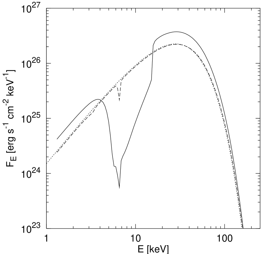
Figure 6: Model spectra for the atmosphere with the magnetic field perpendicular to the surface and the smaller scaleheight $H=1$ cm. In the case of the $z=z_{0,1}$ injection (long-dashed line), the vacuum feature nearly disappears, while for the $z=z_{0,2}$ case (solid line), the lower bound of the feature moves to higher energy compared with the model with $H=10$ cm.

As was noted in Bulik & Miller (1997), the exact shape of the spectra and the vacuum feature depends also on other parameters than the injection depth, like the magnetic field strength, the scaleheight and the pair fraction. Figures 3 and 6-7 show the effects of changing the atmosphere scaleheight $H$. With increasing $H$ the vacuum feature broadens, the upper energy bound on the feature remains roughly constant, whereas the lower bound moves to lower energies. This is due to the fact that the typical density gradients are smoother when $H$ is large and hence the optical depth through the vacuum resonance increases. The depth of the proton cyclotron line also increases with scaleheight, which is especially marked for the lower production depth $z_{0,1}$. Note that in this case the vacuum feature and the proton line are considerably influenced by the value of $H$ and, in particular, they may be virtually nonexistent for low scaleheights (e.g. Fig. 6).

The spectra presented are essentially independent of viewing direction except for the angles near $\theta\approx 90^{o}$. In this case, the vacuum resonance disappears (see eqs 30-31) which results in the lack of the absorption-like feature in the spectrum. Further, the depth of the proton line is considerably enhanced and the high-energy tail is reduced, which is due to geometric effects.

Figure 8 shows integrated photon spectra for the model with the magnetic field tilted at the angle $45^{o}$ to the neutron star surface ($B=10^{15}$ G) and the atmosphere scaleheight $H=10$ cm. The overall shape of the spectrum does not significantly differ from the one obtained in the model with perpendicular magnetic field, also shown in Figure 8 for comparison. The angular dependence of radiation can be conveniently analyzed in a coordinate system $(\tilde{x},\tilde{y},\tilde{z})$ in which the $\tilde{z}$-axis is directed along magnetic field. In this system, the vacuum resonance disappears when $\tilde{\theta}=90^{\circ}$, where $\tilde{\theta}$ is the wavevector inclination angle to the magnetic field. At a given propagation angle $\tilde{\theta}$ and growing azimuthal angle $\tilde{\phi}$ (the azimuthal angle is set to zero at the $-\tilde{y}$-axis and $\bf B$ lies in the $yz$-plane), the depth of the proton line and the vacuum feature increases and the lower bound on the feature moves to lower energies. This is due to geometric effects, since at a given propagation angle $\tilde{\theta}$ and growing $\tilde{\phi}$, the physical depth to the top of the atmosphere increases.

4.2 Polarization characteristics

Since the low-cross-section mode makes the main contribution to the photon flux emerging from the optically thick neutron star atmosphere, the observed radiation is expected to acquire strong linear polarization. As noted in §2.2, the polarization pattern of this radiation is modified around the critical points in the system of vacuum and proton-electron plasma, which influence the frequency and angular dependences of normal mode polarization characteristics.

Figure 9 shows an example behavior of ellipticities ${\cal P}_{j}$ and position angles $\chi_{j}$ of the two normal modes in the vicinity of the critical points in a plasma of density $\rho_{0,1}$ ($z=z_{0,1}$). The labeling of the modes is arbitrary. The behavior of ${\cal P}_{j}$ and $\chi_{j}$ near the first critical frequency $\hbar\omega_{c,1}=\hbar\omega_{V,1}=3.38$ keV is different from the behavior at the second critical frequency $\hbar\omega_{c,2}=\hbar\omega_{Bp}=6.4$ keV, because for the photon propagation direction we chose $\theta=78.5^{o}$ ($\cos\theta=0.2$) $\theta>\theta_{c,1}=48^{o}$ ($\cos\theta_{c,1}=0.67$) but $\theta<\theta_{c,2}=89.95^{o}$ ($\cos\theta_{c,2}=8\cdot 10^{-4}$) (see §2.2). At the passage through the first critical frequency the sign of ${\cal P}_{j}$ changes, but the position angles remain essentially the same. The modes are nearly linearly polarized (they become exactly linear at $\omega_{c,1}$) except around $\omega_{c,1}$, where they acquire weak elliptical polarization in the frequency range where $|q|$ is small and $|p|$ is close to unity. This also results in the small nonorthogonality of the modes around $\omega_{c,1}$. In the vicinity of the second critical frequency the normal mode polarization is strongly elliptical. The sign of ${\cal P}_{j}$ remains the same but the position angles jump by $\pm\pi/2$ and coincide at $\omega_{c,2}$. Note also the jump by $\pi$ in the position angle of the low-cross-section mode at energy close to $\omega_{c,2}$. It occurs at the point where parameter $q$ diverges asymptotically ($|q|\gg 1$) and has opposite sign at both sides of the asymptote while at the same time $p$ crosses zero (compare eqs 33-34). Note that the ellipticity is not influenced in this case (see also, e.g., Pavlov & Shibanov (1979) and Bulik & Pavlov (1996) for a discussion of the energy dependence of the polarization characteristics). With growing density, $\theta_{c}$ corresponding to $\omega_{c}=\omega_{Bp}$ is approximately constant, whereas the critical angle corresponding to the vacuum resonance changes. However, at densities at which $\omega_{Bp}\approx\omega_{V}$ the critical angles disappear.

Figure 10 shows the variation of the linear polarization fraction $F_{Q}=<Q>/I$ with photon frequency at the two values of the propagation angle, for the atmosphere model with $H=10$ cm, magnetic field perpendicular to the surface, and the production depths at $z=z_{0,1}$ (Fig. 10a) and $z=z_{0,2}$ (Fig. 10b), respectively. The radiation flux is essentially linearly polarized. Small deviations from linearity appear near the critical frequencies and especially for photons propagating nearly along the direction of the magnetic field. For the case presented in Figure 10a, the decoupling depth is very close to the production depth $z_{0,1}$ (see Fig. 4) at all photon energies, and the location of the critical points is approximately as depicted in Figure 9. Decoupling depths of photons in the model with the production depth located at $z=z_{0,2}$ span a wide range of $z$ between $\sim z_{0,1}$ and $z_{0,2}$, which spreads the deviation of polarization from linearity over the frequency range corresponding to the width of the vacuum feature.

5 DISCUSSION

We have presented a series of Monte Carlo calculations of the atmospheres in the $10^{15}$ G magnetic field. We took into account the electron scattering, the proton scattering, and the free-free absorption. The temperature of the atmosphere is taken to be constant at $10$ keV. The typical variations of the temperature with the optical depth in the difference scheme calculations are weak, $T\approx\tau^{1/4}$ for $\tau\gg 1$ (Özel, 2001; Ho & Lai, 2001). Therefore our assumption of uniform $T$ does not affect the results significantly. The main effect of including the temperature profile of this type would be to increase the flux at the high-energy part of the spectrum (see, e.g., for the emission in quiescence Ho & Lai, 2001, 2003) We investigate in detail the effects of the vacuum resonance and the proton cyclotron resonance in the spectra. We find that the critical frequencies in the normal modes disappear at the density when the vacuum frequency overlaps the proton cyclotron resonance.

In our treatment of the radiative transfer we have neglected the effects of mode conversion (Lai & Ho, 2002, 2003). Mode conversion may occur when photon traverses a layer of varying density and encounters the vacuum resonance. At energies for which the vacuum resonance layer is optically thick in the extraordinary mode, the photon will be scattered or absorbed, which in our method is taken into account. Thus the mode conversion effects do not alter the results in this energy range. In the range of energies where the vacuum resonance layer is optically thin, the low-cross-section mode photon may change its polarization to the high-cross-section one and be absorbed. This effectively increases the optical depth through the resonance layer. Thus the major effect of including the mode conversion effects would be to extend the vacuum absorption-like feature further to the low energies. This effect has also been noted in Lai & Ho (2002).

We confirm the existence of a wide vacuum feature in the spectra. Bulik & Miller (1997) suggested that the feature appears as a consequence of the Comptonization effects. We found that it is formed also in an absorption-dominated atmosphere, which means that the formation of the vacuum feature is a general property expected to occur in spectra of magnetar atmospheres. The vacuum feature appears if the plasma density at the photon production depth is large enough. When the scaleheight is increased, the vacuum feature becomes more prominent since the optical depth through the resonant layer increases (see the estimates in Bulik & Miller (1997)). We have found that the approximate boundary of the density-scaleheight space region where the vacuum absorption-like feature appears in the spectrum can be estimated as $\rho_{inj}>200(H/1{\rm cm})^{-0.26}$g cm^-3, where $\rho_{inj}$ is the density at which photons are injected into the atmosphere. Thus the vacuum feature should be prominent in magnetar spectra provided photons are produced at sufficiently large optical depths and the atmosphere scaleheight is large enough. This second condition might be fulfilled for SGR bursts, since during the burst the atmosphere is probably lifted by radiation pressure and plasma is confined by the strong magnetic field. We do not expect a significant absorption-like feature in the SGR spectra in quiescence. In this case the effective temperature is $T\approx 10^{6}$ K and the vacuum feature would appear only as a broad depression in the exponentially falling high-energy tail, as shown in Ho & Lai (2003) and Özel (2001, 2003).

We find that the proton resonance appears as a narrow line on a wider background. This line is due to the proton resonance itself. The broad background line appears because the presence of the proton resonance affects the normal mode polarization vectors in a broad frequency range around it, which in turn influences the opacities.

We also calculate a model atmosphere with a magnetic field tilted at an angle of $45^{\circ}$ to the surface normal. The spectrum in this case is very similar to the one obtained for the model with perpendicular magnetic field. Such field configurations are important when considering radiation emitted from the entire surface of the star. Our result shows that the spectrum in the tilted field case can be well approximated by the the spectra calculated in the simpler case of the field perpendicular to the surface. This is an independent confirmation of the earlier results obtained in the diffusion approximation for the pulsar-type magnetic fields (see, e.g., Pavlov et al., 1995). For the magnetar-type fields, the spectra for the field tilted at $90^{\circ}$ were shown to be similar to the $0^{\circ}$ case in the Monte Carlo simulations by Bulik & Miller (1997), and in the diffusion approach by Ho & Lai (2001).

We present the polarization of the outgoing radiation. It is essentially linear and the influence of the critical frequencies around the vacuum and proton resonances is very small. For the case of the small production depth $z=z_{0,1}$, the effects of the vacuum resonance appear as deviations from the linear polarization near $\omega_{V}$, especially at the angles close to the direction of $\bf B$. If the injection depth is large, $z=z_{0,2}$, the effects of the vacuum resonance are spread around the width of the feature, as photons arrive to the observer from regions of different densities. The proton cyclotron resonance causes similar distortions from linear polarization at $\omega_{Bp}$, regardless of the production depth.

SGR spectra in outbursts have been first analyzed in the hard X-ray range above $15$ keV and the typical optically thin thermal bremsstrahlung (OTTB) temperatures were found to be in the range of $20$ to $40$ keV (Aptekar et al., 2001). The first analysis of the SGR spectra extending to $5$ keV have been performed for the case of SGR 1806-20 by Laros et al. (1986) and Fenimore et al. (1994). They found that the low energy spectrum was inconsistent with the extension of the OTTB spectra to the lower energies. Strohmayer & Ibrahim (1998) analyzed the RXTE observations of SGR 1806-20 and came up with a similar conclusion. SGR 1900+14 was observed by HETE-2, and Olive et al. (2003) have shown that the low energy spectrum is also qualitatively similar. It was not consistent with an OTTB model, and was modeled by the two blackbody spectra. Recently Feroci et al. (2004) have analyzed several bursts detected from SGR 1900+14 by Beppo SAX in 2001, and found that the OTTB model works fine above $15$ keV but overestimates the flux in the lower-energy range. They tried several alternative models and found the acceptable fits with the two blackbodies with temperatures of $\sim 3$ keV and $10$ keV, and the respective radii of $13$ and $2$ km. We note that such a behavior of the spectrum resembles the presence of a broad vacuum feature. Our model spectra fall below the underlying thermal distribution around $\sim 10$ keV. A double peaked spectrum as shown in, e.g., Figure 7 could well be modeled as two blackbodies with the temperatures differing by a factor of a few. We suspect that these might be the hints of the existence of the vacuum polarization feature in the spectra of SGR bursts. However, in order to definitely claim the detection of such a feature one would have to perform the data analysis using the appropriate model spectra.

Appendix A PLASMA POLARIZATION TENSORS

The general form of the plasma dielectric tensor $\epsilon_{ab}^{(pl)}$ which includes the contribution from both the scattering and free-free absorption processes was given by, e.g, Pavlov & Shibanov (1979). Rewriting their expressions in the coordinate system with the magnetic field along the $z$-axis, and the wavevector in the $yz$-plane at an angle $\theta$ to the magnetic field, we obtain for the plasma polarization tensors components ($s=e,p$ for electrons and protons):

$$\Pi_{xx}^{s} = \frac{\omega(\omega+{\rm i}\gamma_{\perp,s})}{(\omega+{\rm i}\gamma_{\perp,s})^{2}-\omega_{Bs}^{2}},$$ (A1)

$$\Pi_{yy}^{s} = \frac{\omega(\omega+{\rm i}\gamma_{\perp,s})[\omega+{\rm i}\gamma_{\parallel,s}\cos^{2}\theta(1+2\sin^{2}\theta)-{\rm i}\gamma_{\perp,s}\sin^{2}\theta\cos 2\theta]}{(\omega+{\rm i}\gamma_{\parallel,s})[(\omega+{\rm i}\gamma_{\perp,s})^{2}-\omega_{Bs}^{2}]},$$ (A2)

$$\Pi_{zz}^{s} = \frac{\omega(\omega+{\rm i}\gamma_{\perp,s})[\omega+{\rm i}\gamma_{\parallel,s}\cos^{2}\theta\cos 2\theta+{\rm i}\gamma_{\perp,s}\sin^{2}\theta(1+2\cos^{2}\theta)]-\omega\omega_{Bs}^{2}}{(\omega+{\rm i}\gamma_{\parallel,s})[(\omega+{\rm i}\gamma_{\perp,s})^{2}-\omega_{Bs}^{2}]},$$ (A3)

$$\Pi_{xy}^{s} = \frac{{\rm i}\omega\omega_{Bs}}{(\omega+{\rm i}\gamma_{\perp,s})^{2}-\omega_{Bs}^{2}},$$ (A4)

$$\Pi_{xz}^{s} = 0,$$ (A5)

$$\Pi_{yz}^{s} = \frac{-{\rm i}\omega(\omega+{\rm i}\gamma_{\perp,s})(\gamma_{\perp,s}-\gamma_{\parallel,s})\sin 2\theta\cos 2\theta}{2(\omega+{\rm i}\gamma_{\parallel,s})[(\omega+{\rm i}\gamma_{\perp,s})^{2}-\omega_{Bs}^{2}]},$$ (A6)

and

$$\Pi_{yx}^{s}=-\Pi_{xy}^{s},\;\;\Pi_{zx}^{s}=\Pi_{xz}^{s},\;\;\Pi_{zy}^{s}=\Pi_{yz}^{s}.$$ (A7)

The above expressions take into account the influence the strong magnetic field has on the effective frequencies of electron-proton collisions, which then depend on photon polarization. Thus the longitudinal and transverse damping rates are $\gamma_{\parallel,s}=\gamma_{\parallel,cs}+\gamma_{rs}$ and $\gamma_{\perp,s}=\gamma_{\perp,cs}+\gamma_{rs}$, respectively, where the radiative widths $\gamma_{rs}=(2/3)(e^{2}/m_{s}c^{3})\omega^{2}$ and the corresponding collision frequencies $\gamma_{\parallel,cs}=(\sigma_{a}g_{\parallel}/\sigma_{T})\gamma_{rs}$ and $\gamma_{\perp,cs}=(\sigma_{a}g_{\perp}/\sigma_{T})\gamma_{rs}$ (see also Pavlov & Panov, 1976), with $\sigma_{a}$ given by equation (51) and magnetic Gaunt factors $g_{\parallel,\perp}$. When only scattering processes are considered, $\gamma_{\parallel,s}=\gamma_{\perp,s}=\gamma_{rs}$, plasma polarization tensors become diagonal in the rotating coordinates and take the form as given by equation (26).

Figure 1: (a) Scattering and absorption cross-sections as a function of energy at the density $\rho=\rho_{0,1}\simeq 220$ g cm^-3 (corresponding to $z_{0,1}=10H$) and propagation angle $\theta=48^{\circ}$ ($\cos\theta=0.67$). The solid lines show the total (electron + proton) scattering cross-sections for both the high- and the low-cross-section mode. The individual contributions to the total cross-section in the extraordinary mode from electron and proton scattering are shown by dotted and dash-dotted lines, respectively. Note that the vacuum resonance at $\hbar\omega_{V}\simeq 3.38$ keV only slightly affects the proton scattering cross-section. The absorption cross-sections for the two polarization modes are shown by the dashed lines. (b) The mode switching probabilities: low to high mode (dashed line) and high to low mode (solid line).

Figure 2: The dependence of the optical depth on the physical depth in the atmosphere with $H=10$ cm and the magnetic field perpendicular to the surface, for the propagation angle of $48^{\circ}$. The vertical lines denote the photon injection depths in our model simulations, and the numbers next to the curves indicate photon energies in keV. Panel (a) shows the region of photon energies around $\hbar\omega_{V,1}$, while (c) illustrates the range around $\hbar\omega_{V,2}$. The energy range around the proton resonance $\hbar\omega_{Bp}=6.4$ keV, where the vacuum resonance disappears, is shown in (b). Panel (d) illustrates the energy region above the resonances.

Figure 3: Model spectra at the top of the atmosphere for the case of the magnetic field perpendicular to the surface and the scaleheight $H=10$ cm. The dotted line is the input Planck spectrum with $kT=10$ keV. The solid line represents the case of $z=z_{0,2}$ injection, while the long-dashed line corresponds to the case of $z=z_{0,1}$. The spectra for the model without protons are also presented for comparison: dot-dashed line is for $z=z_{0,2}$, and short-dashed line for $z=z_{0,1}$.

Figure 4: The mean decoupling depths for the photon propagation angle of $48^{\circ}$ and for the two production depths we consider: $z=z_{0,1}$ (a) and $z=z_{0,2}$ (b) ($H=10$ cm). Note the difference in vertical scales. In the case of the $z=z_{0,2}$ injection, the vacuum and the proton resonances blend each other.

Figure 5: Model spectra for the atmosphere with $H=10$ cm and the magnetic field perpendicular to the surface in the case when vacuum polarization effects are turned off: dot-dashed line is for $z=z_{0,2}$, and short-dashed line for $z=z_{0,1}$. For reference, we also present the spectra from Fig. 3 for the model with proton and vacuum effects included.

Figure 7: Model spectra for the atmosphere with the magnetic field perpendicular to the surface and the larger scaleheight $H=100$ cm. The slowly changing density gradients increase the influence of vacuum effects for both production depths: $z=z_{0,1}$ (long-dashed line) and $z=z_{0,2}$ (solid line).

Figure 8: Model spectra for the atmosphere with the magnetic field tilted at an angle of $45^{\circ}$ with respect to the surface normal and the scaleheight $H=10$ cm. The $z=z_{0,1}$ case (long-dashed line) is practically indistinguishable from the model with perpendicular field (short-dashed line). For the larger injection depth, $z=z_{0,2}$ (solid line), the vacuum feature is slightly shifted to the higher energies, as compared to the case with perpendicular field (dot-dashed line).

Figure 9: The dependence of the normal mode ellipticities and position angles on photon frequency near the vacuum resonance (left) and the proton resonance (right). The extraordinary (low-cross-section) mode is the one with $\chi\approx\pi/2$. Thus, the labeling of the modes as extraordinary and ordinary does not follow the continuous lines. The photon propagation angle is $\theta=78.5^{\circ}$ and $z=z_{0,1}$.

Figure 10: The deviations from linear polarization, $1-|F_{Q}|$, for the atmosphere with the magnetic field perpendicular to the surface and the standard scaleheight $H=10$ cm for the injection depth $z=z_{0,1}$ (a) and $z=z_{0,2}$ (b). The solid line corresponds to the propagation angle $\theta\approx 8^{\circ}$, close to the direction of the magnetic field, and the dashed line is for $\theta\approx 46^{\circ}$.

References

- Aptekar et al. (2001) Aptekar, R. L., Frederiks, D. D., Golenetskii, S. V., Il’inskii, V. N., Mazets, E. P., Pal’shin, V. D., Butterworth, P. S., & Cline, T. L. 2001, ApJS, 137, 227
- Bezchastnov et al. (1996) Bezchastnov, V. G., Pavlov, G. G., Shibanov, Y. A., & Zavlin, V. E. 1996, in AIP Conf. Proc. 384, Gamma-Ray Bursts: 3rd Huntsville Symposium, ed. C. Kouveliotou, M. F. Briggs, &G. J. Fishman (Woodbury: AIP), 907
- Bulik et al. (1992) Bulik, T., Meszaros, P., Woo, J. W., Hagase, F., & Makishima, K. 1992, ApJ, 395, 564
- Bulik & Miller (1997) Bulik, T., & Miller, M. C. 1997, MNRAS, 288, 596
- Bulik & Pavlov (1996) Bulik, T., & Pavlov, G. G. 1996, ApJ, 469, 373
- Fenimore et al. (1994) Fenimore, E. E., Laros, J. G., & Ulmer, A. 1994, ApJ, 432, 742
- Feroci et al. (2004) Feroci, M., Caliandro, G. A., Massaro, E., Mereghetti, S., & Woods, P. M. 2004, ApJ, 612, 408
- Gavriil et al. (2002) Gavriil, F. P., Kaspi, V. M., & Woods, P. M. 2002, Nature, 419, 142
- Gnedin & Pavlov (1974) Gnedin, Yu. N., & Pavlov, G. G. 1974, Sov. Phys. JETP, 38, 903
- Ho & Lai (2001) Ho, W. C. G., & Lai, D. 2001, MNRAS, 327, 1081
- Ho & Lai (2003) Ho, W. C. G., & Lai, D. 2003, MNRAS, 338, 233
- Ho et al. (2003) Ho, W. C. G., Lai, D., Potekhin, A. Y., & Chabrier, G. 2003, ApJ, 599, 1293
- Hurley (2000) Hurley, K. 2000, in AIP Conf. Proc. 526, Gamma-ray Bursts: 5th Huntsville Symposium, ed. R. M. Kippen, R. S. Mallozzi, & G. J. Fishman (Melville: AIP), 763
- Isenberg et al. (1998) Isenberg, M., Lamb, D. Q., & Wang, J. C. L. 1998, ApJ, 505, 688
- Kouveliotou et al. (1998) Kouveliotou, C., et al. 1998, Nature, 393, 235
- Lai & Ho (2002) Lai, D., & Ho, W. C. G. 2002, ApJ, 566, 373
- Lai & Ho (2003) Lai, D., & Ho, W. C. G. 2003, ApJ, 588, 962
- Laros et al. (1986) Laros, J. G., Fenimore, E. E., Fikani, M. M., Klebesadel, R. W., & Barat, C. 1986, Nature, 322, 152
- Mazets et al. (1979) Mazets, E. P., Golentskii, S. V., Ilinskii, V. N., Aptekar, R. L., & Guryan, I. A. 1979, Nature, 282, 587
- Mereghetti (2001) Mereghetti, S. 2001, in AIP Conf. Proc. 599, X-ray Astronomy: Stellar Endpoints, AGN, and the Diffuse X-ray Background, ed. N. E. White, G. Malaguti, & G. G. C. Palumbo (Melville: AIP), 219
- Mészáros (1992) Mészáros, P. 1992, High-Energy Radiation from Magnetized Neutron Stars (Chicago: Univ. Chicago Press)
- Meszaros & Nagel (1985) Meszaros, P., & Nagel, W. 1985, ApJ, 298, 147
- Miller & Bulik (1996) Miller, M. C., & Bulik, T. 1996, in AIP Conf. Proc. 384, Gamma-Ray Bursts: 3rd Huntsville Symposium, ed. C. Kouveliotou, M. F. Briggs, &G. J. Fishman (Woodbury: AIP), 956
- Olive et al. (2003) Olive, J.-F., et al. 2003, in AIP Conf. Proc. 662: Gamma-Ray Burst and Afterglow Astronomy 2001: A Workshop Celebrating the First Year of the HETE Mission, 82
- Özel (2001) Özel, F. 2001, ApJ, 563, 276
- Özel (2003) Özel, F. 2003, ApJ, 583, 402
- Paczynski (1992) Paczynski, B. 1992, Acta Astronomica, 42, 145
- Pavlov & Panov (1976) Pavlov, G. G., & Panov, A. N. 1976, Sov. Phys. JETP, 44, 300
- Pavlov & Shibanov (1979) Pavlov, G. G., & Shibanov, Yu. A. 1979, Sov. Phys. JETP, 49, 741
- Pavlov et al. (1980) Pavlov, G. G., Shibanov, I. A., & Iakovlev, D. G. 1980, Ap&SS, 73, 33
- Pavlov et al. (1995) Pavlov, G. G., Shibanov, Y. A., Zavlin, V. E., & Meyer, R. D. 1995, in The Lives of the Neutron Stars, ed. M. A. Alpar, U. Kiziloglu, & J. van Paradijs (Boston: Kluwer), 71
- Potekhin & Chabrier (2003) Potekhin, A. Y., & Chabrier, G. 2003, ApJ, 585, 955
- Strohmayer & Ibrahim (1998) Strohmayer, T. E., & Ibrahim, A. 1998, in AIP Conf. Proc. 428, Gamma-Ray Bursts: 4th Huntsville Symposium, ed. C. A. Meegan, R. D. Preece, & T. M. Koshut (Woodbury: AIP), 947
- Thompson & Duncan (1995) Thompson, C., & Duncan, R. C. 1995, MNRAS, 275, 255
- Tsai & Erber (1975) Tsai, W., & Erber, T. 1975, Phys. Rev. D, 12, 1132
- Ventura et al. (1979) Ventura, J., Nagel, W., & Meszaros, P. 1979, ApJ, 233, L125
- Wang et al. (1989) Wang, J. C. L., Wasserman, I. M., & Salpeter, E. E. 1989, ApJ, 338, 343
- Zane et al. (2001) Zane, S., Turolla, R., Stella, L., & Treves, A. 2001, ApJ, 560, 384