Reionization History from Coupled CMB/21cm Line Data

Abstract

We study CMB secondary anisotropies produced by inhomogeneous reionization by means of cosmological simulations coupled with the radiative transfer code CRASH. The reionization history is consistent with the WMAP Thomson optical depth determination. We find that the signal arising from this process dominates over the primary CMB component for $l\lower 2.15277pt\hbox{$\;\buildrel>\over{\sim}\;$}4000$ and reaches a maximum amplitude of $l(l+1)C_{l}/2\pi\simeq 1.6\times 10^{-13}$ on arcmin scale, i.e. $l$ as large as several thousands. We then cross-correlate secondary CMB anisotropy maps with neutral hydrogen 21cm line emission fluctuations obtained from the same simulations. The two signals are highly anti-correlated on angular scales corresponding to the typical size of H$\scriptstyle\rm II\$regions (including overlapping) at the 21cm map redshift. We show how the CMB/21cm cross-correlation can be used to: (a) study the nature of the reionization sources, (b) reconstruct the cosmic reionization history, (c) infer the mean cosmic ionization level at any redshift. We discuss the feasibility of the proposed experiment with forthcoming facilities.

1 Introduction

The Wilkinson Microwave Anisotropy Probe (WMAP) has provided strong evidence for an optical depth to Thomson scattering of $\tau_{e}\sim 0.17\pm 0.04$ (the uncertainty quoted for this number depends on the analysis technique employed), based on the measured correlation between Cosmic Microwave Background (CMB) temperature and polarization on large angular scales (e.g. Kogut et al. 2003). If the reionization process is described as instantaneous and homogeneous, this corresponds to a reionization redshift $z_{ion}\sim 17\pm 5$. More probably, reionization went through a highly inhomogeneous phase (e.g. Ciardi et al. 2000; Gnedin 2000; Miralda-Escudé, Haehnelt & Rees 2000; Ciardi, Stoehr & White 2003, CSW; Sokasian et al. 2003; Ricotti & Ostriker 2004), which ended only when the individual H$\scriptstyle\rm II\$regions overlapped completely. In this case, the reionization process should have left an imprint on the CMB. In fact, the modulation of the ionization fraction, playing a similar role to the density modulation from the non-linear Vishniac effect, leads to anisotropies at sub-degree scales (e.g. Bruscoli et al. 2000; Benson et al. 2001; Gnedin & Jaffe 2001; Santos et al. 2003). In addition to temperature anisotropies, Thomson scattering introduces a polarization signal in the CMB spectrum. The detection of anisotropies in the temperature/polarization power spectrum is an invaluable tool to discriminate between different sources of ionizing photons and reionization histories (e.g. Bruscoli, Ferrara & Scannapieco 2002; Holder et al. 2003; Naselsky & Chiang 2004).

An alternative way to probe the end of the cosmic ‘dark ages’ is through 21cm tomography. From the pioneering work of Field (1959), it has been suggested that the neutral hydrogen in the Intergalactic Medium (IGM) and in gravitationally collapsed systems may be detectable in emission or absorption against the CMB at the frequency corresponding to the redshifted 21cm line associated with the spin-flip transition of the hyperfine levels of neutral hydrogen. The inhomogeneities in the density field, ionized hydrogen and spin temperature produce signatures both in the angular and in the redshift space. Different signatures have been investigated, ranging from the 21cm line emission induced by the ‘cosmic web’ (Madau, Meiksin & Rees 1997; Tozzi et al. 2000), the neutral hydrogen surviving reionization (e.g. Ciardi & Madau 2003; Furlanetto, Sokasian & Hernquist 2004; Furlanetto, Zaldarriaga & Hernquist 2004) or the minihalos with virial temperatures below $10^{4}$ K (e.g. Iliev et al. 2002), to the 21cm lines generated in absorption against very high-redshift radio sources by the neutral IGM (Carilli, Gnedin & Owen 2002) and by intervening minihalos and protogalactic disks (Furlanetto & Loeb 2002).

In this paper, we compute the CMB temperature anisotropies due to an inhomogeneous reionization history obtained from radiative transfer simulations consistent with WMAP observations (Ciardi, Ferrara & White 2003, hereafter CFW). Moreover, we cross-correlate them with the expected 21cm emission maps obtained by Ciardi & Madau (2003, hereafter CM) for the same simulations, and discuss how the cross-correlation can be used to reconstruct the reionization history and to constrain the nature of ionizing sources. Our work is similar in spirit to the recently published study by Cooray (2004), although that work is based on a simplified analytical description of the reionization process. This might be the reason for which our conclusions differ from those obtained by Cooray (see Section 6).

The paper is organized as follows. In Section 2 we present the numerical simulations of IGM reionization by CSW and CFW, and in Section 4 the results of CM on the 21cm emission from such patchy reionization histories are briefly described. In Section 3 we construct and study the maps and the angular power spectra for secondary CMB temperature anisotropies due to the above reionization process, whereas the cross-correlation between CMB and 21cm maps is presented in Section 5. Finally, in Section 6 we summarize and discuss the results.

Throughout the paper we adopt the $\Lambda$CDM “concordance” model with $\Omega_{m}$=0.3, $\Omega_{\Lambda}$=0.7, $h=$0.7, $\Omega_{b}$=0.04, $n$=1 and $\sigma_{8}$=0.9, within the WMAP experimental error bars (Spergel et al. 2003).

2 Numerical Simulations of IGM Reionization

In this Section we briefly describe the numerical simulations of IGM reionization adopted to model the 21cm line emission from neutral IGM and the CMB temperature anisotropies, and refer to CSW and CWF for further details.

A cosmological volume of comoving side 479$h^{-1}$ Mpc has been simulated (Yoshida, Sheth & Diaferio 2001) with the N-body code GADGET (Springel, Yoshida & White 2001). An approximately spherical region with a diameter of about $50h^{-1}$ Mpc has been subsequently “re-simulated” at a higher resolution (Stoehr 2003) with the technique described in Springel et al. (2001, hereafter SWTK). A friends-of-friends algorithm was employed to determine the location and mass of dark matter halos. Gravitationally bound substructures have been identified within the halos with the algorithm SUBFIND (SWTK) and have been used to build the merging tree for halos and subhalos following the prescription of SWTK. A particle mass of $M_{p}=1.7\times 10^{8}h^{-1}$ M_⊙ allows to resolve halos as small as $M\simeq 10^{9}$ M_⊙. The galaxy population has been modeled with the semi-analytic technique described in Kauffmann et al. (1999) and implemented as in SWTK. For each of the simulation output we compile a catalogue of galaxies containing for each galaxy, among other quantities, its position, mass and star formation rate.

A cube of comoving side $L=20h^{-1}$ Mpc has been cut from the high resolution spherical subregion to model the details of the reionization process, using the radiative transfer code CRASH (Ciardi et al. 2001; Maselli, Ferrara & Ciardi 2003) to follow the propagation into the IGM of the ionizing photons emitted by the simulated galaxy population. Several sets of radiative transfer simulations have been run in CSW and CFW, with different choices for the galaxy emission properties. The ones used here are labeled S5 (‘late’ reionization case) and L20 (‘early’ reionization case), and adopt an emission spectrum typical of Pop III stars, a Salpeter Initial Mass Function (IMF) and an escape fraction of ionizing photons $f_{esc}=5\%$ (S5) and a Larson IMF with $f_{esc}=20\%$ (L20). For details and discussion on the choice of parameters we refer to CSW and CFW. The S5 and L20 simulations give a reionization redshift of $z_{ion}\approx 8$ and $\approx 13$, respectively. In addition, they provide the redshift evolution and the spatial distribution of ionized/neutral IGM and have been used to model both the H$\scriptstyle\rm I\$21cm line emission (see Sec. 4) and the CMB temperature anisotropies (see Sec. 3).

3 Secondary CMB Anisotropies

The solution of the Boltzmann equation for the present value of the perturbation of the photon temperature $(\delta T/T)_{\rm CMB}$, along the line of sight (los) $\hat{\gamma}$, can be written as:

$$\left(\frac{\delta T}{T}\right)_{\rm CMB}(\hat{\gamma})=\tau_{0}\int_{0}^{1}{\frac{d\eta}{\eta^{4}}}\chi({\bf x},\eta)\hat{\gamma}\cdot{\bf v}({\bf x},\eta),$$ (1)

where $\eta=\int(1+z)dt$ is the conformal time and $\tau_{0}=n_{e,0}\sigma_{T}\eta_{0}c$, with $n_{e,0}$ being the present free electron density, $\sigma_{T}$ the Thomson cross section and $c$ the light speed. The quantities $\chi({\bf x},\eta)$ and ${\bf v}({\bf x},\eta)$ are the ionization fraction and the peculiar velocity in units of $c$, respectively, calculated at position ${\bf x}=\hat{\gamma}(\eta_{0}-\eta)$ and conformal time $\eta$.

In principle, a map of temperature anisotropies can be simply obtained by integrating eq. (1) along each los passing trough random slices of the simulation boxes. However, the periodic simulation boundary conditions would artificially enhance the anisotropy signal by a non-negligible factor (Gnedin & Jaffe 2001). To prevent this spurious effect, we randomly flip and transpose each simulation box around any of its six edges, hence breaking the fictitious correlations introduced by the computational method. We consider 30 (65) simulation outputs from $z=18.7$ to complete reionization, i.e. $z\approx 13$ ($z\approx 8$) for the L20 (S5) model. The output redshifts are optimized to completely cover the path between the initial and final redshift of the simulation. Although this method might now somewhat underestimate the true anisotropy signal as we miss the contribution of scales larger than the box, the results constitute a solid lower limit to such quantity. In addition, we emphasize that the size of our box ($L=20h^{-1}$ Mpc) is one of the largest used up to now for reionization studies, hence making the large-scale missing power a less severe effect.

The dimension of the map is set by the angle subtended by the simulation box at the highest redshift; for the adopted cosmology $\theta_{max}\approx 9.25$ arcmin. The spatial information on the ionization fraction is obtained from the radiative transfer simulations, whereas the peculiar velocity field is provided by the $N$-body simulation. We repeat the above integration for a random realization with the same volume-averaged value of the ionization fraction $\chi$. A map of the temperature fluctuations due to ionized patches (i.e. the inhomogeneous part) is derived by subtracting the two maps. The result is shown in Fig. 2 for the S5 (top left panel) and the L20 (top right panel) model.

3.1 Anisotropy distribution

The statistics of temperature anisotropy can be analyzed in terms of spherical harmonics, $Y_{lm}$:

$$\left(\frac{\delta T}{T}\right)_{\rm CMB}(\hat{\gamma})=\sum_{l=1}^{\infty}\sum_{m=-l}^{l}a_{lm}Y_{lm}(\hat{\gamma}),$$ (2)

The angular power spectrum, $C_{l}$, is then defined as:

$$C_{l}\equiv<|a_{lm}^{2}|>=\frac{1}{2l+1}\sum_{m}a_{lm}^{2}.$$ (3)

There is a strict relation between the probed angular scale $\theta$ and the multipole $l$ in the formula above, $\theta\simeq 180/l$ degrees. Therefore the extension and resolution of our maps sets an interval in $l$ in which our analysis is meaningful, i.e. $4000\leq l\leq 1.67\cdot 10^{5}$, corresponding to $1/3$ of the map and the pixel scale, respectively. To analyze the maps and obtain the angular power spectrum we use the software package HEALPix(Górski, Hivon & Wandelt 1999). The results are shown in Fig. 1 together with the primary CMB power spectrum from WMAP data fitting (Spergel et al. 2003). The signal due to patchy reionization dominates the primary CMB power spectrum for $l\lower 2.15277pt\hbox{$\;\buildrel>\over{\sim}\;$}4000$ and reaches a maximum amplitude of $\approx 1.6\times 10^{-13}$. The amplitude in the two models is comparable. The power spectrum obtained here is in agreement with that derived by Gnedin & Jaffe (2001), and it is roughly an order of magnitude smaller than the one calculated by Santos et al. (2003) via a semi-analytical model. A last aspect which is worth commenting is the fact that the anisotropy keeps a rather flat level up to the highest significant multipoles. That is the indication that the secondary anisotropy from reionization keep their structure at least up to the arcsecond scale.

Figure 1: Primary CMB power spectrum from WMAP data fitting (dotted line; Spergel et al. 2003), together with the angular power spectra from patchy reionization in the L20 (solid) and S5 (dashed) model.

3.2 Comments on observability

The detection of the signal from patchy reionization requires high sensitivity experiments that can reach large multipole numbers, since the peak of the power spectrum is expected to be at $l$ of the order of few $\times 10^{3}$. These characteristics are within the capability of the next generation of millimeter wavelength interferometers like ALMA, ACT, or CQ. For example, ALMA is expected to reach sensitivities of 2 $\mu$K rms for a $1^{\prime}$ beam with 1 $h$ integration up to 2 arcmin scale, thus appearing as a perfect instrument to search for signature of inhomogeneous reionization.

However, to measure the power spectrum from patchy reionization, several other astrophysical signals must be cleaned out from the maps. In particular, the main foregrounds in the angular range discussed here are the thermal Sunyaev-Zel’dovich (SZ) and the Poisson noise from faint point sources. Thermal SZ is expected to be negligible, at least after multifrequence cleaning, for observations at 217 GHz (Zhang, Pen & Trac 2004). More important is the foreground from unresolved IR and radio sources, which is several orders of magnitude above the reionization signal at $l\lower 2.15277pt\hbox{$\;\buildrel>\over{\sim}\;$}{\rm few}\times 10^{4}$. Luckily, this foreground contamination can be described in terms of a simple power-law (White & Majumdar 2003). Thus, a foreground measurement at $l\approx 10^{4}$ would allow to extrapolate its value at lower $l$, where it can be subtracted to obtain a clean reionization signal. For this reason, multifrequency observations are particularly suited to subtract such foreground contamination. For this technique to be successful though, a good knowledge of the instrumental noise is required.

4 21 cm radiation from neutral IGM

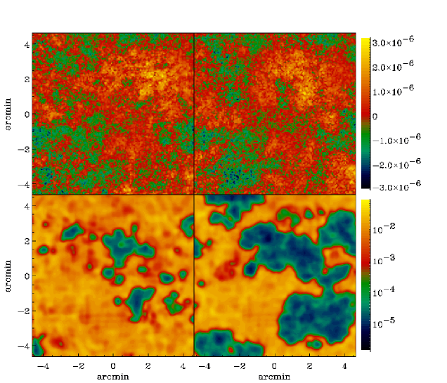
Figure 2: Top panels: map of CMB temperature fluctuations, $(\delta T/T)_{\rm CMB}$, due to patchy reionization for the S5 (left panel) and the L20 (right panel) model. The maps measure $\approx 9.25$ arcmin on a side. Lower panels: maps of differential antenna temperature, $(\delta T/T)_{\rm 21cm}$, from 21cm line emission for the S5 (left panel) and the L20 (right panel) model, at an observed frequency (redshift) $\nu\approx 115$ MHz ($z\approx 11$) and $\nu\approx 90$ MHz ($z\approx 14.5$), respectively. The maps have been derived assuming a bandwidth $\Delta\nu=1$ MHz and measure $\approx 9.25$ arcmin on a side.

The 21cm hyperfine transition of neutral hydrogen in the IGM provides a powerful probe to study the era of cosmological reionization. In this paper we use the results from the numerical simulation of CM, that we briefly describe in this Section. We refer to the above paper for further details.

The emission of the 21cm line is governed by the spin temperature, $T_{S}$. In the presence of a CMB radiation with $T_{\rm CMB}=2.725(1+z)$ K, $T_{S}$ quickly reaches thermal equilibrium with $T_{\rm CMB}$, and a mechanism is required that decouples the two temperatures. While the spin-exchange collisions between hydrogen atoms are too inefficient for typical IGM densities, Ly$\alpha$ pumping contributes significantly by mixing the hyperfine levels of neutral hydrogen in its ground state via intermediate transitions to the $2p$ state. If a Ly$\alpha$ background $\lower 2.15277pt\hbox{$\;\buildrel>\over{\sim}\;$}9\times 10^{-23}(1+z)\,$ergs cm^-2 s^-1 Hz^-1 sr^-1 is present at redshift $z$, Ly$\alpha$ pumping will efficiently decouple $T_{S}$ from $T_{\rm CMB}$. CM find that the diffuse flux of Ly$\alpha$ photons produced by the same sources responsible for the IGM reionization, satisfies the above requirement from $z\approx 20$ to the time of complete reionization. As the IGM can be easily preheated by primordial sources of radiation (e.g. Madau, Meiksin & Rees 1997; Chen & Miralda-Escudé 2003), the universe will, most likely, be observable in 21cm emission at a level that is independent of the exact value of $T_{S}$. Variations in the density of neutral hydrogen (due to either inhomogeneities in the gas density or different ionized fraction) will appear as fluctuations of the sky brightness of this transition, and allow, in principle, to map the history of reionization.

Using the numerical simulations described in Section 2, CM have studied the evolution of the 21cm line emission expected from those reionization histories. In particular, they have derived maps and fluctuations of brightness temperature at different redshifts (i.e. observed frequencies) in both the S5 and L20 model. The S5 model predicts a peak in the amplitude of the expected rms brightness fluctuations at an observed frequency (redshift) $\nu\approx 115$ MHz ($z\approx 11$), whereas in the L20 the peak is at $\nu\approx 90$ MHz ($z\approx 14.5$). In both models, the overall amplitude of the signal at its peak is $\langle\delta T_{rms}^{2}\rangle^{1/2}\approx 10-20$ mK at angular scales $\theta\approx 5$ arcmin (see CM for details). In Fig. 2 maps of differential antenna temperature, $(\delta T/T)_{\rm 21cm}\equiv\delta T_{b}/T_{\rm CMB}(0)$, are shown for the S5 (lower left panel) and the L20 (lower right panel) model at the peak frequencies. The maps have been derived from the simulations of reionization described in Section 2 assuming a bandwidth $\Delta\nu=\nu\Delta z/(1+z)=1$ MHz and measure $\approx 9.25$ arcmin on a side.

5 CMB/21 cm Cross-correlation

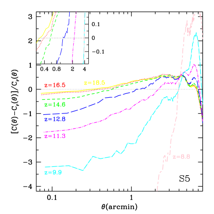
Figure 3: Cross-correlation between the CMB secondary anisotropy map and the 21cm maps at different redshifts (marked by different line styles) for a bandwidth $\Delta\nu=1$ MHz. In the small panel, a zoom of the region in which the transition from anti-correlation to correlation occurs is shown. The subscript r refers to the random cross-correlation. Model S5.

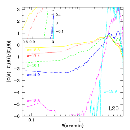
Figure 4: The same of Fig. 3, but for Model L20. Note that lines refer to different redshifts.

CMB secondary anisotropies from patchy reionization are expected to be highly anti-correlated with 21cm line emission temperature fluctuations on scales smaller than the angle subtended by typical H$\scriptstyle\rm II\$regions at the redshift of the 21cm emission. To quantify this effect, we compute the cross-correlation between the CMB and the 21cm map at redshift $z$ as:

$$C(\theta,z)=\sum_{i=1}^{N_{\rm CMB}}\sum_{j=1}^{N_{\rm 21cm}}\frac{1}{N_{\theta}}\left[\left(\frac{\delta T}{T}\right)_{\rm CMB}(i)\left(\frac{\delta T}{T}\right)_{\rm 21cm}(j,z)\right],$$ (4)

where $N_{\rm CMB}$ ($N_{\rm 21cm}$) is the number of pixels in the CMB (21cm) map. The components of $C(\theta,z)$ are then binned according to the separation angle $\theta$ between the two lines of sight passing through the pixels $i$ and $j$ of the 21cm map at redshift $z$. $N_{\theta}$ is the number of values falling in $[\theta,\theta+\theta_{min}]$, where $\theta_{min}$ is the angular dimension of the cell. We repeat this procedure for a random binning. The results are shown in Fig. 3 and 4 for the S5 and L20 model, respectively. The subscript r refers to the random cross-correlation. The small box in the top-left corner shows a zoom of the region in which the majority of the curves first pass through a zero point, i.e. from anti-correlation to correlation.

As expected, we find that the two signals are highly anti-correlated below a characteristic angular scale, $\theta_{0}$, except for the highest redshift where only a very small fraction of the volume is ionized (line at $z=18.5$). The amplitude of the anti-correlation signal increases with decreasing redshift until reionization is almost completed. At any given redshift the model L20 shows a stronger anti-correlation signal, as reionization proceeds more rapidly, and a larger $\theta_{0}$, as a result of the relative larger (on average) H$\scriptstyle\rm II\$region sizes. In fact, the angular scale $\theta_{0}$ indicates the typical dimension of the H$\scriptstyle\rm II\$regions (including overlapping) at that redshift and allows, in principle, to reconstruct the reionization history and to discriminate among different reionization models and sources (e.g. quasars or massive Pop III stars versus more standard stars).

The redshift evolution of the angular scale $\theta_{0}$ is shown in Fig. 5; labels there indicate the typical comoving dimension of the corresponding H$\scriptstyle\rm II\$regions in units of Mpc/$h$. As the evolution of $\theta_{0}$ reflects the growth of H$\scriptstyle\rm II\$regions, the value of $\theta_{0}$ at a given redshift is very different for the two models considered. In general, this result can be used to discriminate among different ionizing sources as H$\scriptstyle\rm II\$regions produced by quasars or massive Pop III stars typically tend to be larger than those digged by more standard stars. Moreover, as the redshift evolution of $\theta_{0}$ reflects the growth of H$\scriptstyle\rm II\$regions, non-monotonic reionization histories would result in a more complex behavior for $\theta_{0}$. For example, in case of a double-reionization (e.g. Cen 2003; Wyithe & Loeb 2003) we expect that $\theta_{0}$ increases until the first reionization is completed. Then, once the ionizing emissivity drops and the IGM partially recombines, $\theta_{0}$ should decrease or remain constant, and eventually grow again when the second reionization takes place.

From our simulations it is also possible to derive a relation between the measured value of $\theta_{0}$ and the volume averaged hydrogen ionization fraction in the computational volume. This relation is shown in Fig. 6. From there we see that the two quantities are positively correlated. It is also worth noticing that a 50% mean ionization level is characterized by $\theta_{0}\approx 3^{\prime}$ independently of the adopted reionization model: identifying this epoch is crucial as it corresponds to the redshift at which most of the CMB secondary anisotropies are produced and it provides a sensible definition of the reionization redshift for prompt reionization models often adopted for practical purposes (Bruscoli, Ferrara & Scannapieco 2002). Moreover, the $\theta_{0}$ - $x_{e}$ relation appears to be quite insensitive to the details of the reionization model, thus providing a robust mapping between the correlation function and the mean ionization level at each epoch.

The results in Fig. 3 and 4 have been derived assuming a bandwidth for 21cm line observations of $\Delta\nu=1$ MHz. Although a smaller bandwidth, e.g. 0.1 MHz, would substantially increase the intensity of 21cm line emission (CM), it does not significantly affect the estimates of the cross-correlation (Fig. 5).

In conclusion, we find that the cross-correlation between secondary anisotropy in the CMB and 21cm emission maps can be a useful tool to follow the reionization process and to give constraints on the nature of the ionizing sources. Moreover, the cross-correlation, combining information obtained by different experiments, can be used to maximize the signal from the reionization process with respect to instrumental noise, systematic errors in the measures, and astrophysical foregrounds.

Figure 5: Redshift evolution of the angular scale at which the transition between anti-correlation and correlation takes place in the L20 (upper curves) and S5 (lower) models. The labels report the typical comoving dimension of the corresponding H$\scriptstyle\rm II\$regions (including overlapping) in units of Mpc/$h$. The 21cm maps have been obtained assuming a bandwidth $\Delta\nu=1$ MHz (solid lines) and 0.1 MHz (dotted).

Figure 6: Relation between the zero-point angle of the cross-correlation function and the mean ionization fraction in the simulation box for the S5 (left panel) and L20 (right) models. The 21cm maps have been obtained assuming a bandwidth $\Delta\nu=1$ MHz (solid lines) and 0.1 MHz (dotted).

6 Summary

We have calculated the secondary anisotropies in the CMB temperature power spectrum produced by inhomogeneous reionization from radiative transfer simulations consistent with WMAP observations. We find that the signal arising from this process dominates over the primary CMB component for $l\lower 2.15277pt\hbox{$\;\buildrel>\over{\sim}\;$}4000$ and reaches a maximum amplitude of $l(l+1)C_{l}/2\pi\simeq 1.6\times 10^{-13}$ on arcminute angular scales, i.e. $l$ as large as several thousands. We then cross-correlated the secondary CMB anisotropy maps with 21cm line emission fluctuation maps for the same reionization simulations. As expected, the two signals are highly anti-correlated on angular scales corresponding to the typical size of H$\scriptstyle\rm II\$regions (including overlapping) at the redshift of the 21cm map. The cross-correlation and, in particular, the redshift evolution of the angular scale at which the transition between anti-correlation to correlation takes place, can be used: (a) to study the nature of the reionization sources, (b) to reconstruct the cosmic reionization history, (c) to infer the mean cosmic ionization level at any redshift.

Cooray (2004) has studied the correlation signal between CMB temperature anisotropies and 21cm fluctuations by means of an analytical reionization model. He concludes that, contrary to what we have shown, the correlation cannot be seen in the angular cross-power spectrum, due to a geometric cancellation effect between velocity and density fluctuations. However, such cancellation likely occurs due to the assumption made in that paper that the neutral hydrogen fraction depends only on overdensity but not on spatial location. In fact, Cooray writes the neutral hydrogen density as $n_{HI}=x_{H}\bar{n}(1+\delta)$, where $x_{H}$ is the neutral H fraction, $\bar{n}$ is the mean gas density and $\delta$ is the gas overdensity. In a patchy reionization scenario, where the ionized bubbles around luminous sources do not completely fill the cosmic volume, it is clear that this assumption is not correct, as two fluctuations with the same $\delta$ value located either inside a ionized region or outside it will have different $n_{HI}$. Hence, if the patchiness of the reionization can be properly modelled (e.g. through radiative transfer simulations) the degeneracy (and the above cancellation) can be broken. Notice that the largest contribution to the secondary anisotropies come from the epoch when roughly 50% of the cosmic volume is filled with bubbles and where the variance in the relation $n_{HI}-\delta$ is largest.

Planned millimeter wavelength interferometers, like ALMA and ACT, are expected to have sensitivities and angular resolution good enough to measure the signature of inhomogeneous reionization in the CMB maps. However, extracting information on the reionization process from the observed maps can be hampered by the presence of both astrophysical foregrounds and instrumental noise. The same applies to 21cm emission observations (see Di Matteo, Ciardi & Miniati 2004 for a detailed study of the foreground contamination of 21cm maps). Provided that both the CMB and 21cm maps can be cleaned from foreground contamination, the information obtained from a cross-correlation of the two maps is an invaluable tool to study the reionization history and its sources.

References

- [1] Benson, A.J., Nusser, A., Sugiyama, N. & Lacey, C.G. 2001, MNRAS, 320, 153
- [2] Bruscoli M., Ferrara A., Fabbri R., Ciardi B., 2000, MNRAS, 318, 1068
- [3] Bruscoli, M., Ferrara, A. & Scannapieco, E. 2002, MNRAS, 330, L43
- [4] Carilli, C.L., Gnedin, N.Y. & Owen, F. 2002, ApJ, 577, 22
- [5] Cen, R. 2003, ApJ, 591, 12
- [6] Chen, X. & Miralda-Escudè, J. 2003, ApJ, 602, 1
- [7] Ciardi, B., Ferrara, A., Governato, F. & Jenkins, A.: 2000, MNRAS, 314, 611
- [8] Ciardi, B., Ferrara, A., Marri, S. & Raimondo, G. 2001, MNRAS, 324, 381
- [9] Ciardi, B., Ferrara, A. & White, S.D.M. 2003, MNRAS, 344, L7 (CFW)
- [10] Ciardi, B. & Madau, P. 2003, ApJ, 596, 1 (CM)
- [11] Ciardi, B., Stoehr, F. & White, S.D.M. 2003, MNRAS, 343, 1101 (CSW)
- [12] Cooray, A. 2004, astro-ph/0405528
- [13] Di Matteo, T., Ciardi, B. & Miniati, F. 2004, astro-ph/0402322
- [14] Field, G.B. 1959, ApJ, 129, 551
- [15] Furlanetto, S.R. & Loeb, A. 2003, ApJ, 588, 18
- [16] Furlanetto, S.R., Sokasian, A. and Hernquist, L. 2004, MNRAS, 347, 187
- [17] Furlanetto, S.R., Zaldarriaga, M. and Hernquist, L. 2004, astro-ph/0403697
- [18] Gnedin, N.Y. 2000, ApJ, 535, 530
- [19] Gnedin N. Y. & Jaffe A. H., 2001, ApJ, 551, 3
- [20] Gnedin N. Y. & Shandarin S. F., 2002, MNRAS, 337, 1435
- [21] Górski, Hivon & Wandelt, 1999, in Proceedings of the MPA/ESO Cosmology Conference ”Evolution of Large-Scale Structure”, eds. A.J. Banday, R.S. Sheth and L. Da Costa, PrintPartners Ipskamp, NL, pp. 37-42 (also astro-ph/9812350)
- [22] Holder, G.P., Haiman, Z., Kaplinghat, M. & Knox, L. 2003, ApJ, 595, 13
- [23] Iliev, I.T., Shapiro, P.R., Ferrara, A. & Martel, H. 2002, ApJ, 572, L123
- [24] Kauffmann, G., Colberg, J. M., Diaferio, A. & White, S. D. M. 1999, MNRAS, 303, 188
- [25] Kogut A. et al., 2003, ApJS, 148, 161
- [26] Madau, P., Meiksin, A., & Rees, M. J. 1997, ApJ, 475, 492
- [27] Maselli, A., Ferrara, A. & Ciardi, B. 2003, MNRAS, 345, 379
- [28] Miralda-Escudé, J., Haehnelt, M. & Rees, M.R., 2000, ApJ, 530, 1
- [29] Naselsky, P. & Chiang, L.-Y. 2004, MNRAS, 347, 795
- [30] Ricotti, M. & Ostriker, J.P. 2004, MNRAS, 350, 539
- [31] Santos M. G., Cooray A., Haiman Z., Knox L., Ma C.-P., 2003, ApJ, 598, 756
- [32] Sokasian, A., Abel, T., Hernquist, L.E. & Springel, V. 2003, MNRAS, 344, 607
- [33] Spergel, D.N. et al. 2003, ApJS, 148, 175
- [34] Springel, V., White, S. D. M., Tormen, G. & Kauffmann, G. 2001, MNRAS, 328, 726 (SWTK)
- [35] Springel, V., Yoshida, N. & White, S. D. M. 2001, NewA, 6, 79
- [36] Stoehr, F. 2003, PhD Thesis, Ludwig Maximilian Universität, München
- [37] Tozzi, P., Madau, P., Meiksin, A. & Rees, M.J. 2000, ApJ, 528, 597
- [38] White M. & Majumdar S., 2004, ApJ, 602, 565
- [39] Wyithe, J.S.B. & Loeb, A. 2003, ApJ, 586, 693.
- [40] Yoshida N., Sheth R.K. & Diaferio A., 2001, MNRAS, 328, 669
- [41] Zhang P., Pen U. & Trac H., 2004, MNRAS, 347, 1224