An Analysis Of Optical Pick–up In SCUBA Data

Abstract

The Sub-millimetre Common User Bolometer Array (SCUBA) at the JCMT employs a chopping and nodding observation technique to remove variations in the atmospheric signal and improve the long term stability of the instrument. In order to understand systematic effects in SCUBA data, we have analysed single–nod time streams from across SCUBA’s lifetime, and present an analysis of a ubiquitous optical pick–up signal connected to the pointing of the secondary mirror. This pick–up is usually removed to a high level by subtracting data from two nod positions and is therefore not obviously present in most reduced SCUBA data. However, if the nod cancellation is not perfect this pick–up can swamp astronomical signals. We discuss various methods which have been suggested to account for this type of imperfect cancellation, and also examine the impact of this pick–up on observations with future bolometric cameras at the JCMT.

1 Introduction

In recent years, millimetre (mm) and sub-millimetre (sub-mm) bolometric cameras have become the focus of much effort. These instruments directly detect thermal emission associated with star formation and have proven useful in studying previously hidden processes in our own galaxy and others to very high redshifts (e.g. Lilly et al. 1999, Dunne & Eales 2001, Johnstone et al. 2001, Ivison et al. 2002, Scott et al. 2002, Chapman et al. 2003). The Submillimetre Common User Bolometer Array (SCUBA; Holland et al. 1999) at the James Clerk Maxwell Telescope (JCMT), with its large aperture and excellent site, has been particularly productive in this field.

Even exploiting a combination of high, dry sites and ‘windows’ in atmospheric opacity, emission due to the atmosphere and telescope’s surroundings is very large compared to astrophysical signals (Archibald et al., 2002). Moreover, it is highly variable on time scales slower than a few Hz. To counteract this, sub-mm telescopes can employ a variety of observing strategies to scan the sky rapidly and take differences to remove the bulk of the atmospheric emission. These techniques put astrophysical signals into an audio frequency band above the atmospheric 1/f knee. Examples of specific observing strategies are those employed by SHARC II (Dowell et al., 2003), which scans the sky in a lissajous pattern, and BLAST (Tucker et al., 2004) and ACT (Kosowsky, 2004), which will scan the entire telescope in azimuth only. SCUBA uses a rapidly moving secondary mirror to chop the beam rapidly and nods the whole telescope more slowly (Holland et al., 1999) while SCUBA2 (which will also be deployed at the JCMT, Holland et al. 2003) intends to employ the DREAM algorithm (Le Poole & van Someren Greve, 1998). In all of these approaches the observation and data reduction processes which cancel atmospheric signals also filter astrophysical signals at large angular scales.

Previous efforts to measure the Sunyaev-Zel’dovich (SZ) effect on the JCMT have failed due to early removal of large angular scale signals during data reduction. Therefore, as part of an effort to measure the SZ effect with SCUBA (Zemcov et al., 2003), we have taken the unorthodox step of considering SCUBA data before subtracting data from adjacent nods. When we do this we find a repetitive signal which is orders of magnitude larger than typical astronomical and even atmospheric signals. Fig. 1 shows an example of this signal.

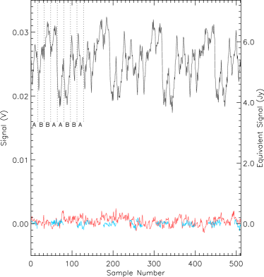
Figure 1: A typical reconstructed SCUBA data series for a $120$ arcsecond chop throw. This particular data set is for bolometer G13 from observation 28 on 1998 June 30. The upper trace shows the time ordered data collected during four consecutive 64 point jiggle patterns. Each sample is $1.024\,$s of data averaged over the chop but there are occasional small gaps in the data series associated with time spent nodding the telescope not shown here. Every bolometer in the array shows a similar pattern which is large, stable, and occurs at the jiggle frequency. In the usual data reduction pipeline successive nod patterns are subtracted and this cancels the repetitive pattern almost completely. This is shown as the blue interrupted trace which represents $A1-B1$, $A2-B2$, $A3-B3$, and $A4-B4$ for the four cycles. There are therefore half as many data points in this double–differenced set as in the raw data, so this trace is plotted only in the $A$ nod position. The lower red (continuous) curve is the residual after subtracting the polynomial model of mirror position discussed below. It is nearly as clean as the blue data set.

We will show that this signal is associated with changes in the orientation of the secondary mirror and presumably arises from altering the amount of thermal emission from the telescope which is received by the bolometer array. Although this signal is present in all SCUBA data we have examined, it generally seems to be removed effectively in the standard surf (Jenness & Lightfoot, 1998) reduction pipeline. However, a period during which nod subtraction does not effectively cancel this pick–up has already been identified by at least one author (Borys et al., 2004).

This signal is synchronized with motion of the secondary mirror, and therefore occurs in the data at a set of audio frequencies overlapping those of astronomical signals. Its presence imposes severe constraints on viable observation strategies and on the required precision of optical control at both the JCMT and similar telescopes. In this paper we present measurements and analysis of this signal with the aim of learning what these constraints are and determining the origin of this signal.

2 Observation of Optical Pick–Up

2.1 SCUBA observation strategies

Holland et al. (1999) and Archibald et al. (2002) provide excellent and extensive reviews of standard SCUBA operations and systematic effects. We review here just enough of the SCUBA observation modes to allow understanding of the pattern shown in Fig. 1.

The JCMT’s beam is chopped on the sky by nutating the secondary mirror at about $7.8\,$Hz in a nearly square wave pattern. The angular separation of the end points of this chop, called the chop throw, is chosen by the observer. The chop is symmetric about the optic axis of the telescope, which is to say that the two endpoints of the chop pattern are each displaced from the optic axis by half the chop throw. The measured difference in intensity between the two endpoints for every bolometer in both arrays is reported at approximately $1\,$Hz. This signal is largely free of the uniform component of atmospheric emission. We will call this differential data the raw time series.

The entire telescope is reoriented periodically to put one end of the chop pattern and then the other on to the nominal source position. This is called nodding the telescope. The difference in intensity between the two nod positions forms a triple difference on the sky: the brightness at the nominal source position minus that at two symmetrically located off-positions. This signal is largely free of the effects of gradients in atmospheric emission. This data set is called the de–nodded or double–differenced data, and is also shown in Fig. 1.

The SCUBA array under fills the focal plane, so the secondary mirror undergoes a slow, small amplitude walk in addition to the movements described above so that over time the sky is fully sampled.

Figure 2: A schematic of the SCUBA jiggle pattern. It is controlled by motion of the secondary mirror, and allows the SCUBA array to fully sample the sky. The central dashed circle shows the full width half maximum (FWHM) beam size associated with the (circled) central triangular point. The peripheral dashed circles show the FWHM of adjacent bolometers in the SCUBA array; SCUBA under samples the sky at any instant. The secondary mirror chops the beam on the sky at $\sim 8\,$Hz between positions separated by a user-defined angle, dwelling for $\sim 1\,$s with one end of the chop on each of the positions shown above. After completing the 16 positions in one quadrant of the pattern the telescope primary mirror nods and the other end of the chop is put onto each of the 16 positions in the same quadrant. Then the second, third, and fourth quadrants of the jiggle pattern are observed in the same way. If the primary mirror nod positions are called $A$ and $B$ and the jiggle pattern quadrants are numbered 1 through 4 as in the figure, a 64 point measurement pattern consists of the following sequence of $16\,$s measurements: $A1\,B1\,B2\,A2\,A3\,B3\,B4\,A4$. This process requires approximately $128\,$s to complete, plus some overhead associated with moving the primary mirror. Notice that the nod frequency of the primary mirror is $\sim 1/32\,$Hz while secondary mirror positions occur at harmonics of $\sim 1/128\,$Hz

Fig. 2 shows the standard 64 point pattern, called a jiggle pattern. The 64 points are split into four quadrants of 16 pointings each and the telescope nods after observing each quadrant. If we label these quadrants 1 through 4, and label the two nod positions as $A$, and $B$, the order of data collection is

$$A1\quad B1\quad B2\quad A2\quad A3\quad B3\quad B4\quad A4\quad A1\dots$$

The pattern repeats every $(16\ \mathrm{Positions})\times(2\ \mathrm{Nods})\times(4\ \mathrm{Quadrants})=128$ samples, requiring slightly longer than 128 seconds to complete one cycle. The sample series also has gaps in time because the primary mirror requires time to move. The order of observing nod $A$ and nod $B$ alternates by quadrant to minimize primary mirror motion. The peak to peak jiggle distance is about 30 arcsec, and the average jiggle distance from the middle of the pattern is about 9 arcsec. Very similar, albeit simpler, motions occur in SCUBA’s $16$ point jiggle pattern and 9 point photometry modes.

Although the SCUBA bolometers are sampled at $128\,$Hz, data are reported as one second averages over the chop; undifferenced data are not saved. In standard operation, two time streams are reported, one for each nod position. Normally, the nod time streams are subtracted from each other ($A1-B1$ etc.), thereby removing a large component of the atmospheric emission and instrumental variation. This double–difference time stream, which consists of the target beam data minus half of each of the two chop positions’ data, is the standard SCUBA data product.

2.2 The jiggle frequency signal

The raw time series in Fig. 1 shows a clear periodicity at 128 samples, indicating emission is modulated by the 128 point jiggle-and-nod pattern. The peak to peak amplitude of the pick–up signal is about $10\,$mV, which is about $10^{4}$ times as large as those arising from the weakest astronomical sources SCUBA is capable of resolving. In order to provide a consistent, if approximate, guide by which to compare these signals to astrophysical sources and thermal effects we have adopted a gain of $210\,$Jy/V throughout this paper. This is consistent with the mean value observed in pre-upgrade SCUBA data (Jenness et al., 2002). With this gain, the amplitude of the pick–up is about $2\,$Jy per beam peak to peak.

In the de–nodded data set there are 16 points in the set $A1-B1$, 16 in the set $A2-B2$, and so on. These points are also plotted in Fig. 1. The amplitude of the pick–up signal has been dramatically reduced and these signals are consistent with a combination of detector and atmospheric noise. We conclude that the source of the pick–up is not modulated by nodding the telescope, and therefore that the pick–up signal is associated with motions of the secondary mirror only.

To check this conclusion, and to quantify the relation, we fit the raw time series to a polynomial in a secondary mirror orientation using elevation, $h$, and azimuth, $A$, coordinates as tracked by bolometer H7’s jiggle offsets, which are nominally zero on the optical axis of the telescope. This basis forms the natural coordinate system for exploring a signal which arises within or around the telescope. We perform a fit independently in $h$ and $A$, using each angle and its derivatives. It is found that the fit does not require cross terms of $A$ and $h$ to describe the data. Our fitting function is therefore

$$\tilde{V}(t)=V_{0}+\sum_{n=1}^{9}\alpha_{n}A^{n}+\sum_{n=1}^{9}\beta_{n}\dot{A}^{n}+\sum_{n=1}^{9}\gamma_{n}\ddot{A}^{n}+\\ \sum_{n=1}^{9}\delta_{n}h^{n}+\sum_{n=1}^{9}\epsilon_{n}\dot{h}^{n}+\sum_{n=1}^{9}\zeta_{n}\ddot{h}^{n}$$ (1)

where $(A(t),h(t))$ is the secondary mirror pointing at time $t$ measured in arcsec, dots denote time derivatives, and the constants $\alpha_{n}$, $\beta_{n}$, $\gamma_{n}$, $\delta_{n}$, $\epsilon_{n}$ and $\zeta_{n}$ are determined from the fit. In practice, these fits are performed independently to $A$ and then $h$ for each bolometer. The number of terms in the fit is arbitrary; we have chosen $n\leq 9$ as the ninth order terms are consistent with zero. If the signal is optical in origin, we expect the $n=1$ term, which corresponds to position, to dominate, while if it is due to pick–up from motors or electrical equipment, higher order terms, corresponding to velocities and accelerations, should dominate. Any pick–up associated with the nod does not affect the time series at the jiggle frequencies, but rather adds a variable DC offset between the two nod positions. When Eq. 1 is fit, the linear terms $\alpha_{1}$ and $\delta_{1}$ are at least an order of magnitude larger than any other term. This fit is therefore consistent with optical pick–up alone; the higher order terms ($n>1$) are included in order to demonstrate that the pick–up pattern can be completely described in terms of the position of the secondary mirror. Further, we find that the pick–up pattern is not constant but varies smoothly with bolometer position (as shown below), which strongly suggests the pick–up is optical and not electrical in origin. Residuals from this fit, $V(t)-\tilde{V}(t)$, are shown in Fig. 1. Just like the de–nodded data, these residuals also show nearly complete elimination of the pick–up signal. In a single data file this cancellation is effective to about one part in 100; unfortunately, to observe weak astrophysical signals in multiple integrations, we require cancellation to better than one part in 3000.

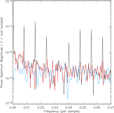
Figure 3: Power spectrum magnitudes (PSM, the modulus of the Fourier transform) of the data shown in Fig. 1. The Fourier transforms have been taken with respect to sample number as the precise mapping between sample number and time is complicated due to small gaps in data collection during normal SCUBA operation. As a guide, 1 sample$\,\simeq 1\,$Hz. The black curve shows the PSM of the raw data set. Note that there is no power at $1/32$ sample^-1, confirming that the pick–up signal is associated with secondary mirror position and not with motion of the primary mirror. The red curve is the PSM of the residual signal after removal of the polynomial model discussed below. This curve contains no power in any of the spikes in the raw data spectrum but faithfully reproduces the PSM everywhere else. The blue curve is the PSM of the double differenced data. Above $1/64$ sample^-1 the PSMs all have comparable power, but at low frequency double differencing produces ‘whitened’ data with about half of the variance of the model subtraction method.

Fourier transforms of the raw data, the de–nodded data, and the residuals from Eq. 1 are shown in Fig. 3. Caution is required when interpreting the transform of the de–nodded data since that data set is sampled differently in time than the other two sets. The raw data shows spikes at harmonics of $1/(128\ \mathrm{samples})$. Notice that the fourth harmonic has no amplitude above the continuum level. This is because the transitions from $A1$ to $B1$, $A2$ to $B2$, etc. occur at the fourth harmonic and nodding does not alter the secondary mirror pattern of motion. All of the harmonic spikes are missing from the power spectra of either the residuals or the de–nodded data. Except at the spikes, the fit residuals match the raw data with high fidelity. Notice that at very low frequencies the de–nodded data is a bit quieter than the residuals are. Presumably noise and large angular scale astronomical signals which occur at low frequencies are removed from the data by nod subtraction.

3 Characterization of the pick–up Signal

In order to understand the severity and prevalence of this signal, data were obtained from both the SCUBA archive, and a dedicated set of observations with very small chop throw in 2003 June. These data were chosen to reflect a sampling of the types of mapping observation commonly performed with SCUBA. We have examined data taken in both 16 point and 64 point jiggle patterns, as well as SCUBA’s photometry mode which uses a small 9 point grid. A variety of chop throw angles between 3 and 180 arcsec have been chosen. In order to reduce possible contamination by astronomical sources, the data sets were selected based on low estimated target flux. An attempt was made to use only fields containing sources with fluxes less than $10\,$mJy, although this criterion was not met in the very small chop throw (less than 15 arcsec) data. A wide range of chop throws are chosen to give a wide sampling of possible SCUBA jiggle map configurations. Also, data straddling the 1999 October SCUBA refit and upgrade are considered. All of the data were taken on photometric nights, $0.04<\tau_{\mathrm{CSO}}<0.09$. In all, over 200 data files of varying lengths spanning nearly all of SCUBA’s operational lifetime have been considered in this analysis.

The data sets considered here have been preprocessed using surf. Programs are called to flat field, de-spike and extinction correct both the double–differenced and single nod time streams; we direct the reader to surf’s documentation for the details of how these procedures are implemented. All of the data discussed here are left at this stage of processing; advanced atmospheric removal has not been implemented.

3.1 Shape of the pattern

For each bolometer in a given observation, the vector

$$\mathbf{g}=\alpha_{1\eta}\hat{A}+\delta_{1\eta}\hat{h},$$ (2)

where the subscript $\eta$ denotes the different bolometers, is closely related to the gradient of $V$ in azimuth-elevation coordinates. Because the linear terms dominate, $\mathbf{g}$ captures almost all of the power in $V$. The units of $\mathbf{g}$ are V arcsec^-1. When the vector field $\mathbf{g}$ is plotted against the location of each bolometer in the focal plane, a clear pattern emerges (Figs. 4 and 5). There is typically a null in the patterns and the magnitude of $\mathbf{g}$ grows with separation from the location of the null in the focal plane.

In order to test whether this signal is only present in the long wavelength SCUBA array, the analysis discussed above is also performed on the short wavelength array (Fig. 4). It is found that the patterns are remarkably similar between arrays, and in particular the null in the pattern occurs at the same position in the two focal planes during any given observation. This implies that this signal originates somewhere in SCUBA’s optical path.

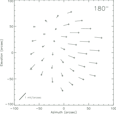
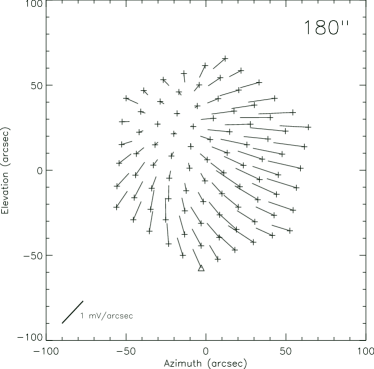
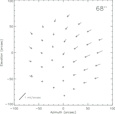
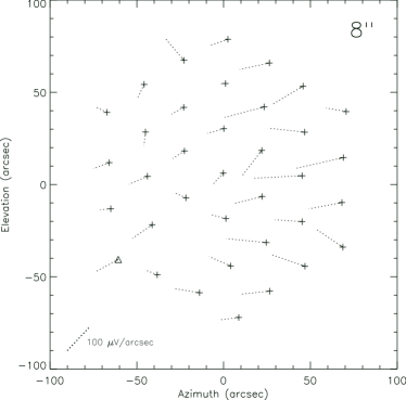
Figure 4: The set of $\mathbf{g}$ for a variety of chop throws (quoted in the upper corner of each plot). The top two plots are comparisons of the $450$/$850\,\mu$m arrays. The plot on the upper left shows the long wavelength array $\mathbf{g}$ from observation 67 on 1999 November 10, and the plot on the upper right shows its short wavelength counterpart. The $\mathbf{g}$ are shown beginning at each bolometer location (‘+’ symbols). Axis units apply only to the bolometer locations, representative scales can be found in the lower left of each plot. Bolometer 1 is marked with a triangle symbol and a scaling for $\mathbf{g}$ is shown in the bottom left of each plot for reference. The patterns are remarkably similar for both arrays, suggesting that the jiggle frequency signal originates in SCUBA’s optical path rather after the dichroic beam-splitter (Holland et al., 1999) or in the electronics. The bottom two plots are for a 68 arcsec chop (observation 119 from 2003 June 14; left) and an 8 arcsec chop (observation 143 from 2003 June 14; right). In 2003, bolometer G9 (number 7) was not operational; its data from that period are not included. These lower plots should be compared with the $180$ arcsec chop throw plot; on a gross scale, the patterns seem to be similar over time. However, smaller chops result in smaller pick–up signals, and the exact pattern changes with each observation.

The pattern in Fig. 4 is a derivative of the optical loading on each bolometer. There appears to be both a divergence and a curl in the pattern, perhaps because Eq. 1 does not employ true partial derivatives, or because the secondary mirror’s orientation and a bolometer’s location in the focal plane are not identically related. In any case, the location of the null in the pattern corresponds to the location of an extremum in the optical loading of the bolometer array. It is striking that in our experience this extremum does not occur at the array centre, which we presume is the symmetry axis of the telescope. However, since the telescope is very difficult to align to arcsec accuracy, it is not unreasonable to expect the symmetry axis to deviate from the array centre by a few tens of arcsec (P. Friberg, private communication).

As a routine part of our Sunyaev-Zel’dovich effect measurements, an aluminum reflector was placed at the cryostat window and observations with large chop throw were performed. This eliminates all optical inputs to the bolometer arrays but leaves electrical pick–up from the various motors and acoustic pick–up intact. The resulting pattern is shown in Fig. 5. The average amplitude of $\mathbf{g}$ is more than two orders of magnitude smaller than without the reflector in place. The pick–up signal must be optical in origin.

The correlated $\mathbf{g}$ patterns occur in every SCUBA data set, and gross features such as the magnitude of the vectors are constant. However, details of each ‘vector field’, such as the centroid, curl, divergence, etc., vary slowly in time. For instance, positional changes in the vector field centroid of tens of arcsec can be tracked over an evening of observation. Furthermore, duplicate observations of the same field performed months apart result in patterns which are quite dissimilar. We believe that this is because a given field’s altitude and azimuth have changed over the intervening time, even though in sky-based coordinates the field’s position is constant. We have had difficulty locating data taken with precisely the same altitude, azimuth and chop throw separated by a suitable interval of time, but surmise that such data would produce very similar patterns if this is an optical pick–up related to ambient radiation in the telescope dome and its surroundings.

3.2 The $\mathbf{\langle|g|\rangle}$ – chop throw distance relation

Careful analysis of Fig. 4 shows that the mean magnitude of the $\mathbf{g}$ vectors, $\langle|\mathbf{g}|\rangle$, is correlated with chop size. The quantity $\langle|\mathbf{g}|\rangle$ and its standard deviation as a function of chop throw are plotted in Fig. 6 for a sampling of data files with different chop throws.

It is observed that the chop size and $\langle|\mathbf{g}|\rangle$ are correlated. While the characteristics of this correlation at modest or large chops are relatively well defined, the signal’s behavior at very small chops is not so clear. In an attempt to clarify whether $\langle|\mathbf{g}|\rangle$ tends to zero at small chop throws, power laws with an offset, $\gamma$

$$\langle|\mathbf{g}|\rangle=\alpha\phi^{\beta}+\gamma.$$ (3)

are fit to data collected with chop throws $\phi$ less than 30 arcsec. The parameters $\alpha$ and $\beta$ are determined from the fit. The results from two of these fits, one with an offset of $\gamma=0\,$V arcsec^-1 and the other with a voltage offset of $\gamma=2.5\times 10^{-5}\,$V arcsec^-1 (this value being arbitrarily chosen for illustrative purposes) are listed in Table 1 and plotted in Fig. 6. The $\chi^{2}$ statistics of these fits are essentially the same. Although the two functions differ in principle, for chop throws of one arcsec the range allowed for the pick–up amplitude is small, from $5$ to $7\,$mJy per arcsec. Even if the pick–up pattern tends to zero at $\phi=0$, coherent mis–pointing during a jiggle observation by a few per cent of the JCMT’s FWHM results in a spurious signal comparable to extra-galactic signals of interest.

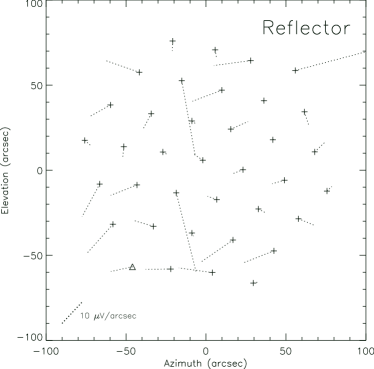
Figure 5: SCUBA pattern with a reflector blocking the dewar aperture (observation 26 from 2002 October 10), with symbols as in Figure 3. The $\mathbf{g}$ are consistent with being random, supporting the claim that the jiggle pick–up originates outside of the SCUBA cryostat.

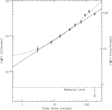
Figure 6: Jiggle frequency signal magnitude as a function of chop throw. The experimental points and their standard errors are shown as diamonds with bars. The lines show power law fits to the smallest four chop throw data points. The best–fitting power law with $\gamma=0\,$V arcsec^-1 offset is shown as the solid line. Also, a power power law with $\gamma=2.5\times 10^{-5}\,$V arcsec^-1 ($\simeq 0.5\,$mJy arcsec^-1) offset is shown as the dot–dash line. The dashed line and arrow at bottom indicate a lower limit to this signal as determined from the reflector data. Because the reflector data’s $\mathbf{g}$ are uncorrelated, $\langle|\mathbf{g}|\rangle$ is an overestimate of the effect in this case, and we plot the limit as half of that calculated. Clearly, the jiggle frequency signal has a substantial amplitude even at small chops. It is very difficult to ascertain the behavior of this signal as the chop throw approaches 0 arcsec.

Table 1: Power law fit parameters.

Fit	$\gamma$	$\alpha$	$\beta$
	(V arcsec-1)	(V arcsec-1)	(arcsec-1)
‘No Offset’	0.0	$2.07\times 10^{-5}$	$0.586$
‘$0.5\,$mJy arcsec-1’	$2.5\times 10^{-5}$	$7.35\times 10^{-6}$	$0.845$

Interestingly, the power laws hold even for the large chop data, although using data at large chop is a poor way to constrain the characteristics of the signal at small chop (this is the motivation for only using the smallest chop data in the fit). While the presence of an offset cannot be ruled out by these data alone, we suspect that the relation is essentially linear and tends to zero at zero chop.

4 Discussion

Finding an optical pick–up signal which depends upon the orientation of the secondary mirror is not a surprise. Moving the secondary mirror alters the electromagnetic cavity formed by the primary and secondary mirrors of the telescope, and also alters the fraction of the beam which intercepts the telescope structure or misses the primary mirror. As has been pointed out, the pattern in Fig. 4 is a derivative of total optical loading on the bolometers. It is quite striking that the observed pattern sometimes corresponds to a minimum loading near to the optical axis, and sometimes to a maximum (as in panels 1 and 3 of Fig. 4).

To compare the observed signals to expectations based on a physical understanding of the telescope first requires conversion of the observations from Jy per beam to an equivalent Rayleigh–Jeans (RJ) temperature. The RJ brightness of a source at $850\,\mu$m is $3.8\times 10^{-17}\,$W m^-2 Hz^-1 str^-1 K^-1, and the solid angle of the JCMT’s primary beam is $\Omega=1.13\times\mathrm{FWHM}^{2}=5.8\times 10^{-9}\,$ str, so

$$\left(\frac{S}{\delta T}\right)=5.8\times 10^{-9}\ \mathrm{str}\\ \times 3.8\times 10^{-17}\,\mathrm{W\ m}^{-2}\ \mathrm{Hz}^{-1}\ \mathrm{K}^{-1}\ \mathrm{str}^{-1}=\\ 22.0\ \mathrm{Jy\ K}^{-1}.$$ (4)

Ideally, this conversion factor would be calculated as an integral over the SCUBA passband (Borys, Chapman & Scott, 1999), which alters the numerical value by a few percent.

The $2.5\,$Jy peak-to-peak signal in Fig. 1 corresponds to a $115\,$mK RJ signal. A more useful number for understanding the emission mechanism is that the chop throw dependent emissivity coefficient $\langle|\mathbf{g}|\rangle$ for a typical chop throw of 60 arc seconds is

$$\langle|\mathbf{g}_{60^{\prime\prime}}|\rangle=50\,\mathrm{mJy\ arcsec}^{-1}=2.2\,\mathrm{mK\ arcsec}^{-1}.$$ (5)

Given that the telescope temperature is typically $270\,$K, this corresponds to a variation in emissivity of $10^{-5}$ per arcsec, averaged over the array.

Several mechanisms could plausibly give emissivity variations which are this high, and we do not know the SCUBA optical illumination pattern well enough to make a definitive distinction. It is certainly possible that several processes are comparable in magnitude. The aluminum reflective surfaces are a few per cent emissive. Their apparent emissivity drops as the mirrors are tilted with respect to each other giving rise to a maximum emission on the optical axis and a variation which is to leading order quadratic in angle. This mechanism will not produce a minimum on axis. However, the measured signal is the difference between the gradients at two chop positions, and thus may have either sign depending on the order of the difference.

The SCUBA plate scale is $\delta d=1.5\,$mm per arcsec (P. Friberg, private communication) so the illumination pattern on the primary moves many cm during routine operation, altering the fraction of the beam spilling off the edge of the mirror and terminating in the telescope enclosure. If $dB/dR$ is the fraction of the total SCUBA response in an annulus of width $dR$ at the edge of the primary of diameter $D=15\,$m, the anticipated signal from variations in beam spill is

$$\frac{dB}{B}=\frac{\pi D\delta d}{\pi D^{2}/4}\frac{dB}{dR}=4\times 10^{-4}\frac{dB}{dR}\,\mathrm{arcsec}^{-1}.$$ (6)

This requires $dB/dR\approx 1$ per cent per mm, which is possible but larger than we expect.

The secondary mirror support structure intercepts $8$ per cent of the beam (P. Friberg, private communication). This coefficient could easily vary by one part in $10^{4}$ per arcsec, which would produce a signal at the observed level. We do not know whether this effect produces a maximum or a minimum near the optic axis. In any case, this very large optical signal is not a malfunction of the telescope, but an unavoidable consequence of employing an observing strategy in which the secondary mirror is moved.

Borys et al. (2004) show that there is a spurious signal at a frequency near to 1 cycle per 16 samples present in SCUBA data collected during much of 2003, and other groups agree (A. Mortrier in preparation, T. Webb in preparation). Published power spectra of this spurious signal look strikingly similar to Fig. 3 given that the authors have not re-ordered their data to be in time-order before implementing a Fourier transformation. We presume that either hardware or software difficulties during that period lead to imperfect nod cancellation, leaving a substantial portion of the secondary mirror-induced pick up signal present in the nominally cleaned data. As a check, we have examined photometry data collected during the same period. In Photometry mode, SCUBA executes a small nine-point grid to account for small errors which might occur in the absolute pointing of the telescope. If the excess noise discussed in Borys et al. (2004) is due to the secondary mirror and poor cancellation, there will be noise at one cycle per nine samples in photometry data. If the noise has a different origin it might well be at the same audio frequency in photometry mode as in jiggle mapping, i.e. one cycle per 16 samples. Fig. 7 shows the power spectrum of a typical bolometer in the first set of photometry data from 2003 we have chosen to examine, and the excess power is clearly near to the frequency of secondary mirror motion for photometry. This broad band of excess noise is absent in data from either 1998 or 2000 which we examined.

Figure 7: The PSM of typical reduced photometry data taken between early to mid 2003 (bolometer I4 from run 57, 2003 February 9). The jiggle frequency spike is present (shown as a dashed line at $f=1/9$ sample^-1), as is a high level of broad-band noise between about $0.05$ and $0.15$ sample^-1. Both are caused by improper nod cancellation; the optical pick–ups are brighter in one nod position than the other, so the difference does not effectively remove common mode contributions. While the photometry mode jiggle frequency is heavily contaminated, no spurious noise is present at the standard jiggle map frequency (the dotted line at $f=1/16$ sample^-1). This is further evidence that the pick–up is due to secondary mirror position.

We conclude that the spurious signal from 2003 is in fact poor cancellation of secondary motion induced pick–up due to poor fine control of the secondary mirror’s postion. This produces large residual signals in the double–differenced data streams. Because the amplitude of the pick–up varies smoothly across the array (e.g. Fig. 4), we have investigated the possibility of using the pattern as a template for removing the signal directly from the data streams. Unfortunately, no bolometer data seem to exhibit a pick–up signal completely described by a gradient term, and it appears that it is not possible to construct a time series that is purely due to the pick–up from this template.

On a positive note, because this signal is bright and stable, it may be possible to use it to provide a short term gain monitor of very high signal to noise ratio in much the same way that Jarosik et al. (2003) use the total power response of their radiometers to obtain a short term gain monitor for WMAP from the system temperature. However, a study of the stability of this signal and the reliability of its dependence on operating parameters is required to implement this strategy.

We do not know how large this effect is 4 arcmin off the optic axis where SCUBA2 intends to have some sensitivity, but we presume from Fig. 6 that it is very large. Furthermore, it is unclear how well this signal can be disentangled from the atmospheric signal without a chopper present in the system. At this point, moving the secondary in any way seems to require nodding or some other symmetric differencing technique to remove the pick–up signal. Unfortunately, the DREAM algorithm currently under consideration for use with SCUBA2 at the JCMT could well be affected by this signal. Furthermore, instruments like THUMPER (Walker et al., 2002) and BOLOCAM (Mauskopf et al., 2000), which may be deployed at the JCMT, will have to develop observation strategies which account for this type of pick–up. These are challenging issues which must be addressed before the next generation of instruments is deployed at the JCMT.

This paper has been typeset from a TeX/LaTeXfile prepared by the author.

References

- Archibald et al. (2002) Archibald E. N. et al., 2002, MNRAS, 336, 1
- Borys, Chapman & Scott (1999) Borys C., Chapman S. C., Scott D., 1999, MNRAS, 308, 527
- Borys et al. (2004) Borys C., Scott D., Chapman S. C., Halpern M., Nandra K., Pope A., 2004, MNRAS, 357, 1022
- Chapman et al. (2003) Chapman S. C. et al., 2003, ApJ, 585, 57
- Dowell et al. (2003) Dowell C. D. et al., 2003, Proceedings of the SPIE, 4855, 73
- Dunne & Eales (2001) Dunne L., Eales S. A., 2001, MNRAS, 327, 697
- Holland et al. (1999) Holland W. S. et al., 1999, MNRAS, 303, 659
- Holland et al. (2003) Holland W. S., Duncan W., Kelly B. D., Irwin K. D., Walton A. J., Ade P. A. R., Robson E. I., 2003, Proceedings of the SPIE, 4855, 1
- Ivison et al. (2002) Ivison R. J. et al., 2002, MNRAS, 337, 1
- Jarosik et al. (2003) Jarosik N. et al., 2003, ApJS, 148 29
- Jenness & Lightfoot (1998) Jenness T., Lightfoot J. F., 1998, in Albrecht R., Hook R. N., Bushouse H. A., eds., ASP Conf. Ser. Vol. 145, Astronomical Data Analysis Software and Systems VII. Astron. Soc. Pac., San Francisco, p. 216
- Jenness et al. (2002) Jenness T., Stevens J. A., Archibald E. N., Economou F., Jessop N. E., Robson E. I., 2002, MNRAS, 336, 14
- Johnstone et al. (2001) Johnstone D., Fich M., Mitchell G. F., Moriarty-Schieven G., 2001, ApJ, 559, 307
- Kosowsky (2004) Kosowsky A., 2004, New Astron. Rev., 47, 939
- Le Poole & van Someren Greve (1998) Le Poole R. S., van Someren Greve H. W., 1998, Proceedings of the SPIE, 3357, 638
- Lilly et al. (1999) Lilly S. J., Eales S. A., Gear W. K. P., Hammer F., Le Fèvre O., Crampton D., Bond J. R., Dunne L., 1999, ApJ, 518, 641
- Mauskopf et al. (2000) Mauskopf P. D. et al., 2000, ASP Conf. Ser. 217. Imaging at Radio Through Submillimetre Wavelengths. Astron. Soc. Pac., San Francisco, p. 115
- Scott et al. (2002) Scott S. E. et al., 2002, MNRAS, 331, 817
- Tucker et al. (2004) Tucker G. S. et al., 2004, Advances Space Res., 33, 1793
- Walker et al. (2002) Walker R. J., Ward–Thompson D., Evans R., Leeks S. J., Ade P. A. R., Griffin M. J., Gear W. K., 2002, Proceedings of the SPIE, 4855, 563
- Zemcov et al. (2003) Zemcov M., Halpern M., Borys C., Chapman S., Holland W., Pierpaoli E., Scott D., 2003, MNRAS, 346, 1179