Complementary constraints on non-standard cosmological models
from CMB and BBN

Abstract

We study metric-affine gravity (MAG) inspired cosmological models. Those models were statistically estimated using the SNIa data. We also use the cosmic microwave background observations and the big-bang nucleosynthesis analysis to constrain the density parameter $\Omega_{\psi,0}$ which is related to the non-Riemannian structure of the underlying spacetime. We argue that while the models are statistically admissible from the SNIa analysis, complementary stricter limits obtained from the CMB and BBN indicate that the models with density parameters with a $a^{-6}$ scaling behaviour are virtually ruled out. If we assume the validity of the particular MAG based cosmological model throughout all stages of the Universe, the parameter estimates from the CMB and BBN put a stronger limit, in comparison to the SNIa data, on the presence of non-Riemannian structures at low redshifts.

I Introduction

Astronomical observations brought important changes in modern cosmology Dodelson (2003). While the type Ia supernovae (SNIa) data are most often employed, the cosmic microwave background (CMB) observations and big-bang nucleosynthesis (BBN) analysis can also be used. They allow the exotic physics of cosmological models to be checked against the observational data Kamionkowski (2002). There is an increasing effort to develop some cosmological and astrophysical tools to search for new physics beyond the standard model.

The metric-affine gravity (MAG) cosmological model with the Robertson-Walker symmetry was investigated by three different groups. First, it was considered the model with triplet ansatz in vacuum Obukhov et al. (1997). Second, it was considered the dilational hyperfluid model Babourova and Frolov (2003). Third, it was shown that on the level of the field equations the special case of the MAG model is equivalent to a model in the Weyl-Cartan spacetime if we choose a model parameter in the special form ($a_{6}=-a_{4}$) Puetzfeld and Chen (2004). Moreover after redefinition of some variables the second and third approach gives the same set of dynamical equations. The analysis of constraints on parameters in the MAG model can be addressed in all three approach, but we adopt the last one proposed by Puetzfeld and Chen Puetzfeld and Chen (2004).

Note that in the model with dust matter on the brane, apart from dark radiation which scales like $a^{-4}$, there is a correction of the type $a^{-6}$ to the Einstein equations on the brane which arise from the influence of a bulk geometry Randall and Sundrum (1999a, b); Godlowski and Szydlowski (2004). The term scaling like $a^{-6}$ also appears in the Friedmann-Robertson-Walker model with spinning fluid Szydlowski and Krawiec (2004). It is possible to establish formally the one to one correspondence between the MAG model and either the Randall-Sundrum brane model when positive values of the non-Riemannian contribution to effective energy is admitted or the spinning fluid filled cosmology when this contribution is negative. However, if one takes the pure Randall-Sundrum type model then there is a constraint on the brane tension parameter coming from the theory itself. The brane tension parameter is not less than about ($100$ GeV)⁴. The MAG model is free from such a theoretical constraint.

In our further discussion we examine the flat models which is motivated by the CMB WMAP observations Kamionkowski et al. (1994) and consider the following formula for the Friedmann first integral

$$\frac{H^{2}}{H_{0}^{2}}=\Omega_{{\rm m},0}a^{-3}+\Omega_{\Lambda,0}+\Omega_{{\rm r},0}a^{-4}+\Omega_{\psi,0}a^{-6}$$ (1)

where $H=d\ln a/dt$ is the Hubble function, $t$ is the cosmological time, $a=a(t)$ is the scale factor, $\Omega_{{\rm m},0}$, $\Omega_{\Lambda,0}$ and $\Omega_{\psi,0}$ are the density parameters for dust matter, the cosmological constant and fictitious fluid which mimics “non-Riemannian effects”, respectively. Their values in the present epoch are marked by the index “0”. All density parameters satisfy the constraint condition

$$\Omega_{{\rm m},0}+\Omega_{\Lambda,0}+\Omega_{{\rm r},0}+\Omega_{\psi,0}=1.$$ (2)

The density parameter for the fictitious fluid is defined as Puetzfeld and Chen (2004)

$$\Omega_{\psi}=\frac{\upsilon}{H^{2}}\frac{\psi^{2}}{a^{6}}$$ (3)

where

$$\upsilon=\frac{\kappa^{2}}{144a_{0}}\left(1-\frac{3a_{0}}{b_{4}}\right).$$

The sign of the parameter $\upsilon$ is undetermined and it can assume both positive and negative values.

II Constraint from the SNIa

Let us start from the reestimation of the models parameters by using the latest sample of SNIa data Riess et al. (2004). The motivation to study the SN constraint is to find the best estimation available from the latest data which gives the narrowest constraint for this method. In the next sections we compare it with constraints obtained from other methods.

Riess et al.’s sample contains 157 type Ia supernovae Riess et al. (2004). We consider the flat model with and without priors on the $\Omega_{\psi,0}$ and $\Omega_{{\rm m},0}$. We assume that the former can be of any value or only nonnegative, and the latter is nonnegative or equal $0.3$ Peebles and Ratra (2003). We estimate the best fits of the model parameters (Table 1). Additionally we find the maximum likelihood estimates with the errors at $2\sigma$ level (Table 2).

Table 1: Best fit estimation of the model parameters from the SNIa data

priors	$\Omega_{{\rm m},0}$	$\Omega_{{\rm r},0}$	$\Omega_{\psi,0}$	$\Omega_{\Lambda,0}$	$\mathcal{M}$	$\chi^{2}$
$\Omega_{\psi,0}\geq 0$; $\Omega_{{\rm m},0}\geq 0$	$0$	$0.14$	$0.012$	$0.848$	$15.945$	$175.75$
$\Omega_{\psi,0}\geq 0$; $\Omega_{{\rm m},0}=0.3$	—	$0$	$0.005$	$0.695$	$15.965$	$177.30$
$\Omega_{{\rm m},0}\geq 0$	$0$	$0.14$	$0.012$	$0.848$	$15.945$	$175.75$
$\Omega_{{\rm m},0}=0.3$	—	$0$	$0.005$	$0.695$	$15.965$	$177.30$
$\Omega_{{\rm m},0}\geq 0$; $\Omega_{{\rm r},0}=0.0001$	$0.16$	—	$0.029$	$0.811$	$15.945$	$175.97$
$\Omega_{{\rm m},0}=0.3$; $\Omega_{{\rm r},0}=0.0001$	—	—	$0.005$	$0.695$	$15.965$	$177.30$

Table 2: Maximum likelihood estimation of the model parameters with $2\sigma$ errors from the SNIa data

priors	$\Omega_{{\rm m},0}$	$\Omega_{{\rm r},0}$	$\Omega_{\psi,0}$	$\Omega_{\Lambda,0}$
$\Omega_{\psi,0}\geq 0$; $\Omega_{{\rm m},0}\geq 0$	$0_{-0.00}^{+0.24}$	$0_{-0.00}^{+0.15}$	$0.009_{-0.009}^{+0.041}$	$0.820_{-0.120}^{+0.100}$
$\Omega_{\psi,0}\geq 0$; $\Omega_{{\rm m},0}=0.3$	—	$0_{-0.00}^{+0.04}$	$0_{-0.000}^{+0.017}$	$0.680_{-0.040}^{+0.020}$
$\Omega_{{\rm m},0}\geq 0$	$0_{-0.00}^{+0.27}$	$0_{-0.00}^{+0.21}$	$0.009_{-0.036}^{+0.042}$	$0.800_{-0.140}^{+0.110}$
$\Omega_{{\rm m},0}=0.3$	—	$0_{-0.00}^{+0.09}$	$\-0.002_{-0.022}^{+0.017}$	$0.680_{-0.060}^{+0.020}$
$\Omega_{{\rm m},0}\geq 0$; $\Omega_{{\rm r},0}=0.0001$	$0.14_{-0.14}^{+0.28}$	—	$0.028_{-0.035}^{+0.038}$	$0.810_{-0.150}^{+0.130}$
$\Omega_{{\rm m},0}=0.3$; $\Omega_{{\rm r},0}=0.0001$	—	—	$0.005_{-0.013}^{+0.013}$	$0.695_{-0.015}^{+0.015}$

We find that that the estimates of the parameter $\Omega_{\psi,0}$ are very close to zero although positive apart of one case when it is zero. We can conclude that the estimate of this parameter is order of magnitude of $0.01$.

To illustrate the results of the maximum likelihood analysis of the model we draw the levels of confidence on Figure 1.

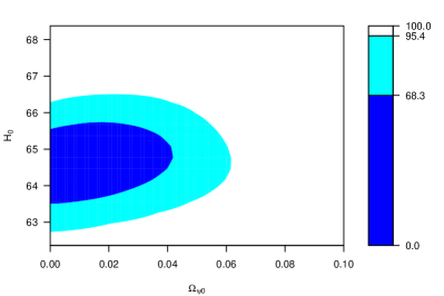
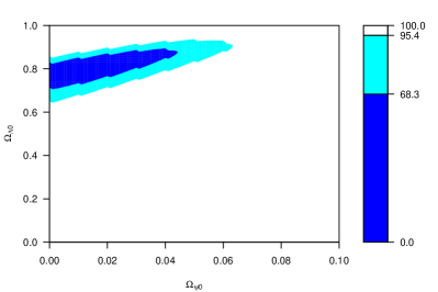
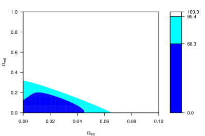
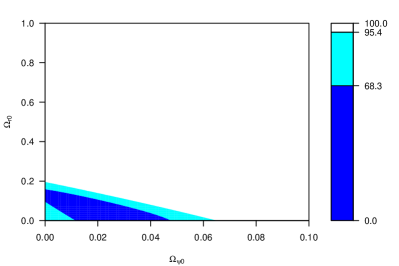
Figure 1: The contours with $1\sigma$ and $2\sigma$ confidence levels for $\Omega_{\psi,0}$ versus $H_{0}$, $\Omega_{\Lambda,0}$, $\Omega_{{\rm m},0}$, and $\Omega_{{\rm r},0}$ from the SNIa data.

The MAG model fits well to SNIa data. We consider the model with any value of $\Omega_{{\rm r},0}$ we obtain the value of $\Omega_{{\rm m},0}$ equal zero as best fit and maximum likelihood estimator, while fixing the small amount radiation ($\Omega_{{\rm r},0}$ Vishwakarma and Singh (2003)) gives the low density matter universe. The estimation of the Hubble constant gives the value close to $65$ km/s MPc.

III CMB peaks in the MAG model

The hotter and colder spots in the CMB can interpreted as acoustic oscillation in the primeval plasma during the last scattering. Peaks in the power spectrum correspond to maximum density of the wave. In the Legendre multipole space these peaks correspond to the angle subtended by the sound horizon at the last scattering. Further peaks answer to higher harmonics of the principal oscillations.

It is very interesting that locations of these peaks are very sensitive to the variations in the model parameters. Therefore, it can be used as another way to constrain the parameters of cosmological models.

The acoustic scale $\ell_{A}$ which puts the locations of the peaks is defined as

$$\ell_{A}=\pi\frac{\int_{0}^{z_{\rm dec}}\frac{dz^{\prime}}{H(z^{\prime})}}{\int_{z_{\rm dec}}^{\infty}c_{s}\frac{dz^{\prime}}{H(z^{\prime})}}$$ (4)

where

$$H(z)=H_{0}\sqrt{\Omega_{{\rm m},0}(1+z)^{3}+\Omega_{{\rm r},0}(1+z)^{4}+\Omega_{\psi,0}(1+z)^{6}+\Omega_{\Lambda,0}}$$ (5)

and $c_{\rm s}$ is the speed of sound in the plasma given by

$$c_{\rm s}^{2}\equiv\frac{dp_{\rm eff}}{d\rho_{\rm eff}}=\frac{\frac{4}{3}\Omega_{\gamma,0}(1+z)+6\Omega_{\psi,0}(1+z)^{3}}{3\Omega_{{\rm b},0}+4\Omega_{\gamma,0}(1+z)+6\Omega_{\psi,0}(1+z)^{3}}.$$ (6)

Knowing the acoustic scale we can determine the location of $m$-th peak

$$\ell_{m}\sim\ell_{A}(m-\phi_{m})$$ (7)

where $\phi_{m}$ is the phase shift caused by the plasma driving effect. Assuming that $\Omega_{{\rm m},0}=0.3$, on the surface of last scattering $z_{\rm dec}$ it is given by

$$\phi_{m}\sim 0.267\left[\frac{r(z_{\rm dec})}{0.3}\right]^{0.1}=0.267\left[\frac{1}{0.3}\frac{\rho_{\rm r}(z_{\rm dec})}{\rho_{\rm m}(z_{\rm dec})}\right]^{0.1}=0.267\left[\frac{1}{0.3}\frac{\Omega_{{\rm r},0}(1+z_{\rm dec})}{0.3}\right]^{0.1}$$ (8)

where $\Omega_{{\rm b},0}h^{2}=0.02$, $r(z_{\rm dec})\equiv\rho_{\rm r}(z_{\rm dec})/\rho_{\rm m}(z_{\rm dec})=\Omega_{{\rm r},0}(1+z_{\rm dec})/\Omega_{{\rm m},0}$ is the ratio of radiation to matter densities at the surface of last scattering.

The CMB temperature angular power spectrum provides the locations of the first two peaks Spergel et al. (2003); Page et al. (2003) and the BOOMERanG measurements give the location of the third peak de Bernardis et al. (2002). They values with uncertainties on the level 1$\sigma$ are the following

$$\ell_{1}=220.1_{-0.8}^{+0.8},\qquad\ell_{2}=546_{-10}^{+10},\qquad\ell_{3}=845_{-25}^{+12}.$$

Using the WMAP data only, Spergel et al. Spergel et al. (2003) obtained that the Hubble constant $H_{0}=72$ km/s MPc (or the parameter $h=0.72$), the baryonic matter density $\Omega_{{\rm b},0}=0.024h^{-2}$, and the matter density $\Omega_{{\rm m},0}=0.14h^{-2}$ which give a good agreement with the observation of position of the first peak.

To find whether cosmological models give these observational locations of peaks we fix some model parameters. Let the baryonic matter density $\Omega_{{\rm b},0}=0.05$, the spectral index for initial density perturbations $n=1$, and the radiation density parameter Vishwakarma and Singh (2003)

$$\Omega_{{\rm r},0}=\Omega_{\gamma,0}+\Omega_{\nu,0}=2.48h^{-2}\times 10^{-5}+1.7h^{-2}\times 10^{-5}=4.18h^{-2}\times 10^{-5}$$ (9)

which is a sum of the photon $\Omega_{\gamma,0}$ and neutrino $\Omega_{\nu,0}$ densities.

Assuming $\Omega_{{\rm m},0}=0.3$ and $h=0.72$ we obtain for the standard $\Lambda$CDM cosmological model the following positions of peaks

$$\ell_{1}=220,\qquad\ell_{2}=521,\qquad\ell_{3}=821$$

with the phase shift $\phi_{m}$ given by (8).

From the SNIa data analysis it was found that the Hubble constant has lower value. Assuming that $H_{0}=65$ km/s MPc (or $h=0.65$), we have $\Omega_{{\rm r},0}=9.89\times 10^{-5}$ from equation (9). In further calculation we take $\Omega_{{\rm r},0}=0.0001$. If we consider the standard $\Lambda$CDM model, with $\Omega_{{\rm m},0}=0.3$, $\Omega_{{\rm b},0}=0.05$, the spectral index for initial density perturbations $n=1$, and $h=0.65$, where sound can propagate in baryonic matter and photons we obtain the following locations of first three peaks

$$\ell_{1}=225,\qquad\ell_{2}=535,\qquad\ell_{3}=847.$$

We find some discrepancy between the observational and theoretical results in this case. Now it is interesting to check whether the presence of the fictitious fluid $\Omega_{\psi,0}$ change the locations of the peaks.

The properties of the fictitious fluid $\Omega_{\psi,0}$ are unknown. In particular, we do not know whether the sound can or cannot propagate in this fluid. But we assume that sound can propagate in it as well as in baryonic matter and photons. We consider both values of the Hubble constant and assume that $h=0.65$ or $h=0.72$. The results of calculations of peak locations and the values of the parameter $\Omega_{\psi,0}$ are presented in Table 3.

Table 3: Values of $\Omega_{\psi,0}$ and location of first three peaks

Hubble constant	$\Omega_{\psi,0}$	$\ell_{1}$	$\ell_{2}$	$\ell_{3}$
$H_{0}=65$ km/s MPc	$3\times 10^{-11}$	$220$	$522$	$825$
	$7\times 10^{-14}$	$220$	$523$	$826$
	$-1.4\times 10^{-10}$	$223$	$530$	$847$
$H_{0}=72$ km/s MPc	$3.7\times 10^{-11}$	$220$	$522$	$823$
	$0$	$220$	$521$	$821$
	$-1.3\times 10^{-10}$	$224$	$530$	$847$

If we choose the $H_{0}=65$ km/s MPc then we obtain the agreement with the observation of the location of the first peak for three non-zero values of the parameter $\Omega_{\psi,0}$. As it is shown on Figure 2 there are two positive and one negative values of this parameter for which the MAG model is admissible.

All these distinguished values of $\Omega_{\psi,0}$ are in agreement with the result obtained from SNIa because the $2\sigma$ confidence interval for this parameter obtained from the SNIa data contains these three points. While the SNIa estimations give the possibility that $\Omega_{\psi,0}$ is equal zero, the CMB calculations seem to exclude this case because the zero value of $\Omega_{\psi,0}$ requires the first peak location at $225$.

If we choose the $H_{0}=72$ km/s MPc than one of positive values of $\Omega_{\psi,0}$ move to zero, while the second one move a little to the right.

We also calculated the age of the Universe in the MAG model. We find that the difference in the age of the Universe is smaller than 1 mln years for all three values of $\Omega_{\psi,0}$. Assuming that $\Omega_{{\rm m},0}=0.3$ the age of the Universe is $14.496$ Gyr for $H_{0}=65$ km/s MPc, and $13.088$ Gyr for $H_{0}=72$ km/s MPc. The globular cluster analysis indicated that the age of the Universe is $13.4$ Gyr Chaboyer and Krauss (2003).

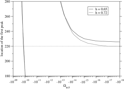
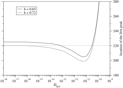
Figure 2: The location of the first peak in function of $\Omega_{\psi,0}$.

IV Constraint from the BBN

It is well known that the big-bang nucleosynthesis (BBN) is the very well tested area of cosmology and does not allow for any significant deviation from the standard expansion law apart from very early times (i.e., before the onset of BBN). The prediction of standard BBN is in well agreement with observations of abundance of light elements. Therefore, all nonstandard terms added to the Friedmann equation should give only negligible small modifications during the BBN epoch to have the nucleosynthesis process unchanged.

In our opinion the consistency with BBN is a crucial issue in the MAG models where the nonstandard term $a^{-6}$ in the Friedmann equation is added (see also discussion in Puetzfeld (2003)). This additional term scales like $(1+z)^{6}$. It is clear that such a term has either accelerated ($\Omega_{\psi,0}>0$) or decelerated ($\Omega_{\psi,0}<0$) impact on the Universe expansion. Going backwards in time this term would become dominant at some redshift. If it would happen before the BBN epoch, the radiation domination would never occur and the all BBN predictions would be lost.

The domination of the fictitious fluid $\Omega_{\psi}$ should end before the BBN epoch starts otherwise the nucleosynthesis process would be dramatically modified. If we assume that the BBN result are preserved in the MAG models we obtain another constraint on the amount of $\Omega_{\psi,0}$. Let us assume that the model modification is negligible small during the BBN epoch and the nucleosynthesis process is unchanged. It means that the contribution of the MAG term $\Omega_{\psi,0}$ cannot dominate over the radiation term $\Omega_{{\rm r},0}\approx 10^{-4}$ before the beginning of BBN ($z\simeq 10^{8}$)

$$\Omega_{\psi,0}(1+z)^{6}<\Omega_{{\rm r},0}(1+z)^{4}\qquad\Longrightarrow\qquad|\Omega_{\psi,0}|<10^{-20}.$$

The values of $\Omega_{\psi,0}\propto 10^{-2}$ obtained as best fits in the SNIa data analysis as well as the smallest nonzero value of $\Omega_{\psi,0}=7\times 10^{-14}$ calculated in the CMB analysis are unrealistic in the light of the above result. If we take into consideration the maximum likelihood analysis of SNIa data we have the possibility that the value of $\Omega_{\psi,0}$ is lower than $|10^{-20}|$ in the $2\sigma$ confidence interval. In the case of the CMB analysis only the value of the Hubble constant close to $72$ km/s MPc gives the zero or close to zero value of $\Omega_{\psi,0}$.

V Conclusion

The paper discusses observational constraint on “energy contributions” arising in certain cosmological models based on MAG. In particular it is focused on the nonstandard term $a^{-6}$. We test this model against the SNIa data, the location of the peaks of the CMB power spectrum, and constraints from the BBN.

The MAG model fits well to SNIa data and the estimations give the amount of fluid $\Omega_{\psi,0}$ to be order of magnitude $0.01$, and the Hubble constant is close to $65$ km/s MPc. Let us note that these results are compatible with constraints from FRIIb radio galaxies and X-ray gas mass fractions Puetzfeld et al. (2005).

The CMB analysis gives that the Hubble constant is $72$ km/s MPc which gives the too low age of the universe in comparison with the age of globular clusters. Taking lower value of the Hubble constant obtained from SNIa estimation resolves the problem of the age. However, the location of the first peak shifts to the right and is in conflict with the observed location. The introducing of the non-Riemannian structure of the underlying spacetime moves the location of the first peak back and this MAG model agrees with the CMB observations. The analysis of the CMB in this model cannot distinguish the character of the fictitious fluid and we do not know whether the parameter $\Omega_{\psi,0}$ is positive or negative.

The absolute values of $\Omega_{\psi,0}$ obtained in the MAG model from the CMB analysis with $h=0.65$ seems to be too large in comparison to the limit obtained from the BBN analysis. Using the BBN analysis we pointed out that the MAG part of the energy density to its present density parameter is of order $10^{-20}$. The limit of this order leads to the conclusion that the MAG model is virtually ruled out. However, we must remember that we insist that the MAG model does not change the physics during and after the BBN epoch. In this context, the merit of the SNIa analysis is its independency from any assumption on physical processes in the early Universe.