Non-LTE Spectra of Accretion Disks Around Intermediate-Mass Black Holes

Abstract

We have calculated the structures and the emergent spectra of stationary, geometrically thin accretion disks around 100 and 1000 $M_{\odot}$ black holes in both the Schwarzschild and extreme Kerr metrics. Equations of radiative transfer, hydrostatic equilibrium, energy balance, ionization equilibrium, and statistical equilibrium are solved simultaneously and consistently. The six most astrophysically abundant elements (H, He, C, N, O, and Fe) are included, as well as energy transfer by Comptonization. The observed spectrum as a function of viewing angle is computed incorporating all general relativistic effects. We find that, in contrast with the predictions of the commonly-used multi-color disk (MCD) model, opacity associated with photoionization of heavy elements can significantly alter the spectrum near its peak. These ionization edges can create spectral breaks visible in the spectra of slowly-spinning black holes viewed from almost all angles and in the spectra of rapidly-spinning black holes seen approximately pole-on. For fixed mass and accretion rate relative to Eddington, both the black hole spin and the viewing angle can significantly shift the observed peak energy of the spectrum, particularly for rapid spin viewed obliquely or edge-on. We present a detailed test of the approximations made in various forms of the MCD model. Linear limb-darkening is confirmed to be a reasonable approximation for the integrated flux, but not for many specific frequencies of interest.

1 Introduction

Intermediate-mass black holes (IMBHs) are black holes more massive than the stellar-mass black holes found in galactic binaries ($\sim 10$ $M_{\odot}$) and smaller than the super-massive black holes found in active galactic nuclei ($\sim 10^{6}$–$10^{9}$ $M_{\odot}$). Whether IMBHs actually exist is at present an open question.

It has been suggested that IMBHs can be found in Ultra-Luminous X-ray sources (ULXs) (Colbert & Mushotzky 1999; Miller & Hamilton 2002; Miller et al 2003). ULXs are off-center point-like X-ray objects in nearby galaxies with luminosities $\sim 10^{39}$-$10^{41}$ erg s^-1 in the 2-10 keV band. First detected in Einstein observations of nearby spiral galaxies (see, e.g. Fabbiano & Trinchieri 1987), the list of known examples grew with ROSAT/HRI observations and has been further extended with Chandra and XMM-Newton data (see, e.g. Colbert & Ptak 2002; Swartz, et al 2002; Stobbart, et al 2004; Nolan et al 2004). Their variability proves that, whatever their nature, they must be very compact (Strickland, et al 2001).

If their power is produced by accretion, and if their X-ray emission is isotropic and sub-Eddington ($L_{E}=1.3\times 10^{38}(M/M_{\odot}$) erg  s^-1), the mass of the central object must exceed a few tens to $10^{4}~{}M_{\odot}$, depending on the individual object. On the other hand, if any of these assumptions are violated, other explanations for these objects are possible. Examples of such models include anisotropic emission (King et al 2001) or radiation pressure-dominated super-Eddington accretion (Begelman 2002), although there at least a few ULXs with X-ray luminosities too high to be explained in this way (see, e.g., the review by Colbert & Miller 2004). Possible constraints on the degree of anisotropy come from observations of nebulae surrounding ULXs, which are often quite symmetric (Pakull & Mirioni 2003; Kaaret et al 2004). In this paper, we explore the possibility that ULXs are, indeed, sub-Eddington accreting intermediate-mass black holes.

Most ULX X-ray spectra can be described as a sum of two components. At low energies (a few hundred eV to several keV), the spectrum is dominated by an apparently thermal component whose characteristic temperature is typically $\simeq 0.2$ kev. On the other hand, at high energies ($\sim 1$ keV – 10 keV), the spectrum is dominated by a power law with photon spectral index in the range 1.7–2.3 (see, e.g. Miller et al 2003, 2004; Roberts, et al 2004). It is the goal of this paper to provide the most complete prediction of the thermal component done to date.

In past work, the thermal component has often been described in terms of the “multi-color disk” (MCD) model (see, e.g. Mitsuda et al 1984; Makishima et al 1986; Shimura & Takahara 1995, etc.). In this model, it is assumed that the total output spectrum of an accretion disk is a sum of spectra from a series of radial rings. In this model’s simplest form, each ring is supposed to radiate as a blackbody with an effective temperature, $T_{eff}$, determined by a thin-disk model. At large radii, $T_{eff}\propto r^{-3/4}$, where $r$ is the radius of a particular ring. In practice, a variety of variants of this model are employed. Sometimes $T_{eff}$ is taken to scale as $r^{-3/4}$ all the way to an inner edge, within which no radiation is produced, and sometimes its radial scaling is taken from more detailed models (employing either Newtonian or relativistic physics) that assume a dissipation cut-off at the innermost stable circular orbit (ISCO). Sometimes the local ring spectra are supposed to be “dilute” blackbodies (see §3.1 for a discussion of the basis of this approximation). Sometimes the intensity distribution is assumed to be isotropic in the fluid frame as in a true blackbody, and sometimes it is supposed to follow a guessed limb-darkening law (Gierlinski et al 2001). Sometimes relativistic Doppler shifts and trajectory-bending are taken into account (Gierlinski et al 2001; Li et al 2004), but not always (e.g. Makishima et al 2000). There has been only a small amount of effort hitherto to predict rather than assume the spectra radiated by individual disk rings. Ross & Fabian 1996, Merloni et al 2000 and Fabian et al 2004 have employed real transfer, but including only Thomson and free-free opacity (the last paper working specifically in the context of intermediate-mass black holes); Davis et al 2004 have employed the same method as we, but applied to disks around lower-mass black holes.

In this paper, we report calculations that predict the spectra of IMBH accretion disks on the basis of complete atmosphere models for each individual radial ring. Assuming a smooth vertical profile, at each radius we solve the equations of hydrostatic balance, statistical equilibrium, radiation transfer, and energy conservation in order to arrive at the emergent intensity in the fluid frame as a function of frequency and angle. All ionization stages of C, N, O, and Fe are included, as well as H and He. Because we do not allow for the sort of intense heating required to make one, our models do not include any hard X-ray-producing corona, even though a significant hard X-ray component is generally seen in ULX spectra. Nonetheless, there can still be mild temperature increases above the photosphere, and we compute any Comptonization taking place there. The absence of a truly hot ($\sim 100$ keV) corona from out model also means we may be underestimating the photoionization rate in the disk’s upper layers. A better treatment of disk coronae and their effects on disk atmospheres must await greater knowledge of their structure. In the last step of our calculation, we apply a transfer function that takes into account all general relativistic effects to obtain the spectrum seen by distant observers as a function of angle from the black hole rotation axis. In order to show clearly what is new about our results, we make a detailed comparison between our predictions and selected variants of the MCD model.

In §2 we describe in some detail how we performed our calculations. Specific results are presented in §3. We discuss these results in §4, with special attention given to checking the quality of the approximations and assumptions made in the MCD model. In §5, we summarize.

2 Description of our Non-LTE disk model

2.1 Accretion disk model

The physics involved in our calculation of the structure and radiation field of an accretion disk around an IMBH is very nearly the same as that described in a series of papers by Hubeny et al. (see, e. g. Hubeny, Lanz 1995; Hubeny, Hubeny 1998; Hubeny, Agol, Blaes, &Krolik 2000; Hubeny, Blaes, Agol, &Krolik 2001). The principal new element in our work is that we apply this model to accretion disks whose central masses are $10^{2}$ and $10^{3}M_{\odot}$. The earlier work focussed on quasars, and therefore considered disks with central masses in the range $10^{6}-10^{9}M_{\odot}$. In an effort parallel to this work, Davis et al 2004 used the same model to study the output spectra from disks accreting onto a $10M_{\odot}$ black hole.

We assume that these disks are axisymmetric, time-steady and geometrically thin. The standard $\alpha$-model of accretion disks (see, e. g. Shakura, Sunyaev 1973; Novikov, & Thorne 1973) is adopted, i.e., in which the vertically averaged viscous stress, $<t_{r\phi}>\equiv h^{-1}\int_{0}^{h}t_{r\phi}dz$, is related to the vertically averaged total pressure, $<P>$, by the Shakura-Sunyaev $\alpha$, $<t_{r\phi}>=\alpha<P>$. In our calculation, the value of $\alpha$ is taken as 0.01, which is close to the result coming from simulations of magneto-rotational instability in unstratified shearing boxes (see, e. g. Balbus & Hawley 1998). Total pressure, which is composed of the gas pressure and radiation pressure, is determined by solving the hydrostatic equilibrium equation neglecting self-gravity and assuming a geometrically thin disk. We further assume that the energy dissipation rate, whose vertically-integrated value varies with radius, is constant per unit mass at any given radius. By ignoring convection and conduction, we also assume that energy transport occurs solely by the vertical flux of radiation. At each ring in our calculation, the effective temperature is (see, e. g. Krolik 1999)

$$T_{eff}=\left[\frac{3GM\dot{M}}{8\pi\sigma r^{3}}R_{R}(r)\right]^{1/4},$$ (1)

where $\sigma$ is the Stefan-Boltzmann constant and $R_{R}(r)$ incorporates both the effect of the net angular momentum flux through the disk and relativistic corrections (see, e. g. Novikov, & Thorne 1973).

The hardest part of the calculation is solving the radiative transfer equation simultaneously with other structural equations. Because we make no ad hoc assumptions about the the emissivities and opacities or the source function in the disk, we have to determine the angle-dependent radiation field and the emissivities and opacities simultaneously. Because we do not assume local thermal equilibrium (LTE), we must solve the statistical equilibrium equations to find the population densities from which the emissivities and opacities can be calculated. However, before starting to solve these equations, information about the radiation field is needed to construct the rates at which radiation induces changes in atomic state populations. To escape this dilemma, we put all of these ingredients into a self-consistent model that treats the disk structure, energy balance, statistical equilibrium and radiation transfer simultaneously.

Besides those considerations about consistency, two other physically important features are added to our model. One is the effect of thermal Comptonization. We incorporate it into our calculation by introducing an angle-averaged Compton source function (see, e. g. Hubeny, Blaes, Agol, &Krolik 2001), which is constructed under the Kompaneets approximation. The other feature is ground-state continuum opacities of all ionization stages in all the elements included (H, He, C, N, O, Fe). We assume solar abundances, as given in Anders & Grevesse 1989.

Finally, we specify the parameters of the four disks whose spectra we compute and give a brief explanation of the flow of calculation. All our disks accrete at a rate yielding $L/L_{E}=0.1$. Two disks are assumed to lie around Schwarzschild (non-rotating) black holes, two around maximal Kerr black holes. By maximal Kerr, we mean $a/M=0.998$, the limiting ratio of angular momentum to mass estimated by Thorne (1974). For each of the black hole spin cases, we calculate the light output from disks surrounding black holes of two different masses, $100M_{\odot}$ and $1000M_{\odot}$. To produce the required luminosity relative to Eddington, the mass accretion rate in the Schwarzschild case is $3.89\times 10^{-9}(M/M_{\odot})M_{\odot}$ yr^-1, whereas it is $6.84\times 10^{-10}(M/M_{\odot})M_{\odot}$ yr^-1 for the extreme Kerr example.

To compute the integrated spectrum as a function of angle from the disk axis, we divide the disks into a series of concentric annuli. The emergent intensity in the fluid frame is computed for each annulus using TLUSTY (Hubeny, Lanz 1995; Hubeny, Blaes, Agol, &Krolik 2001), and these intensities are then combined into frequency- and angle-dependent fluxes using a general relativistic transfer code (Agol 1997). The transfer code includes Doppler shifting and focussing due to the large orbital speeds, gravitational red-shifts, and bending of geodesics. The radial grid for the Schwarzschild case (in terms of gravitational radius $GM/c^{2}$) is $r=$ 6.5, 7.0, 7.5, 8.0, 8.5, 9.0, 9.5, 10, 11, 12, 13, 14, 15, 16, 17, 18, 20, 30, 40, 50, 60, 100, 200; for the extreme Kerr disk it is finer: $r=$ 1.4, 1.5, 1.6, 1.7, 2.0, 2.5, 3.0, 3.5, 4.0, 4.5, 5.0, 5.5, 6.0, 6.5, 7.0, 7.5, 8.0, 8.5, 9.0, 9.5, 10, 11, 12, 13, 14, 15, 16, 17, 18, 19, 20, 25, 30, 35, 40, 45, 50, 60, 70, 80, 90, 100, 120, 140, 160, 180, 200, 250, 300, 350, 400, 450, 500. The inner and outer radii are chosen to be just outside the marginally stable orbit (on the inside) and far enough away (on the outside) to ensure that the portion of the spectrum within a factor of ten in frequency of the peak is fully represented.

2.2 MCD approximation

A significant part of our effort will be contrasting our results with the standard model used in the literature, the multi-color disk (MCD) model. This model was first introduced to explain observed X-ray spectra by Mitsuda et al 1984. The basic idea behind MCD is to assume that the spectrum of an accretion disk around a black hole is simply a superposition of individual black body spectra, each corresponding to a specific radius. Unfortunately, there is a great deal of confusion in the literature because a number of variations of this idea have been used, all under the same name.

Before identifying which version we take as our standard of comparison, we describe these variations, from simplest to most complex. In the very simplest version, the factor $R_{R}(r)$ (eq.(1)) is set equal to unity everywhere. Making no relativistic corrections, one would then predict an observed spectrum $\propto\nu^{1/3}\exp{(-h\nu/kT_{\rm max})}$, where $T_{max}$ is the temperature of the innermost ring (Lynden-Bell & Pringle 1974). This model is sometimes elaborated in any of three directions. First, even in Newtonian physics, the disk effective temperature does not scale $\propto r^{-3/4}$ all the way to the ISCO and then dive abruptly to zero; the net angular momentum flux through the disk leads to a roll-over that begins somewhat outside the ISCO. The run of effective temperature with radius is sometimes adjusted to reflect this. The detailed form of this roll-over can be further refined by considerations of relativity (Novikov, & Thorne 1973; Page, & Thorne 1974). Second, the local spectrum may not be exactly black body. Many (perhaps most) people using the MCD model suppose that Comptonization shifts the peak of the spectrum to higher frequency. This shift is described in terms of a “dilution” or “hardening” factor $f$ so that the mean intensity at the surface of the disk is

$$J_{\nu}=f^{-4}B_{\nu}(fT_{\rm eff}).$$ (2)

This factor is generally taken to be a constant 1.7, independent of circumstance (Shimura & Takahara 1995; Gierlinski et al 2001). Third, some assumption must be made about the angular distribution of the emergent intensity. Sometimes it is taken to be exactly isotropic in the fluid frame, as it would be if the spectrum were precisely thermal. In other cases (e.g., Gierlinski et al (2001)), a specific choice of limb-darkening law is guessed. In Newtonian physics, these choices suffice to determine the angular distribution of the flux. However, relativistic effects lead to angle-dependent Doppler shifts, beaming, gravitational redshifts, and trajectory-bending. Sometimes these are ignored, sometimes included via exact treatments.

In the rest of our paper, if not specified explicitly, the MCD approximation we choose to compare to our results is the one used by Gierlinski et al (2001). They include the general relativistic corrections to both the disk structure and the photon transfer to distant observers; a diluted black body (hereafter, DBB) with $f=1.7$; and a linear limb-darkening law in the fluid frame

$$I_{\nu}^{\rm ff}(\mu)=0.42(1+2.06\mu)f^{-4}B_{\nu}\left(fT_{\rm eff}\right).$$ (3)

3 Results of calculation

In this section we report the main results of our calculation. In subsection §3.1, we study the flux in the fluid frame at selected radii. Next, we employ the GR transfer function and predict the spectra as seen at various viewing angles (§3.2). Limb-darkening is discussed in greater detail in §3.3, where we contrast fluid-frame and observer-frame descriptions. In the last two parts of this section, we study the effects on observed spectra of varying black hole spin (§3.4) and mass (§3.5).

3.1 Spectra in the local fluid frame

We begin by showing how Comptonization and heavy element photoionization opacity affect the spectrum in the fluid frame. To isolate the effects of heavy elements, we also present the results of calculations that include only H and He; these are labelled “H-He disk”, whereas calculations with the full complement of elements are designated “Fe disk”. The results shown in Fig. 1 are for an accretion disk around a maximal Kerr black hole with mass $10^{2}~{}M_{\odot}$. The annuli chosen to plot are $r$=1.6, 6.5, 10, 20, 50, 100 $r_{g}$ with, correspondingly, $T_{\rm eff}(r)$=6.2, 2.8, 2.1, 1.3, 0.68, 0.41 in $10^{6}K$. Here $r_{g}\equiv GM/c^{2}$. Three different predictions for the emergent fluxes from these 6 rings are shown: a true blackbody with $T=T_{\rm eff}(r)$; the spectrum of an H-He disk; and the spectrum of an Fe-disk.

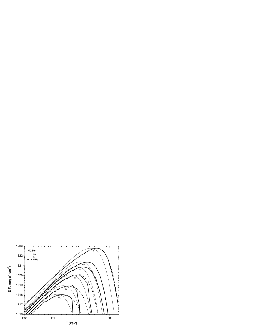
Figure 1: Local flux of H-He and Fe disks in the fluid frame. The central mass of the BH is $10^{2}M_{\odot}$ and it rotates with spin parameter $a/M=0.998$. The thin curves represent the blackbody spectrum with the local effective temperature, while the thick curves show the full atmosphere predictions. Two chemical compositions are displayed, pure H-He atmospheres by dashed curves, solar abundances by solid ones. Six annuli are shown, each of them marked by its radial coordinate in units of $r_{g}$.

The first obvious difference between our NLTE spectra and the blackbody spectra is the blue-shifting of the peak. This shift is largely due to electron scattering blanketing of the thermalization photosphere, an effect most concisely parameterized in terms of the photon-destruction probability $\epsilon_{\nu}\equiv\kappa_{\nu}^{abs}/(\kappa_{\nu}^{abs}+\kappa_{\nu}^{sc})$. Here $\kappa_{\nu}^{abs}$ and $\kappa_{\nu}^{sc}$ are the absorption and scattering opacity, respectively. The surface mean intensity is then (see, Rybicki & Lightman 1979 or Mihalas 1978)

$$J_{\nu}(0)\approx\sqrt{\langle\epsilon_{\nu}\rangle}~{}B_{\nu}(T^{\ast}),$$ (4)

where $T^{\ast}$ is the temperature at the thermalization depth. The local photon-destruction probability in general depends on both density and temperature, and therefore requires an appropriate average for use in equation 4. When $\langle\epsilon_{\nu}\rangle\ll 1$, the spectrum is thermalized at an optical depth $\tau^{*}_{\nu}\simeq(3\langle\epsilon_{\nu}\rangle)^{-1/2}$. The physical effect underlying equation 4 is that a large ratio of scattering to absorption opacity leads to a thick scattering layer between the thermalization photosphere and the surface, suppressing the output. When this occurs in an isothermal atmosphere, the resulting spectrum is called a “modified blackbody”.

In a H-He disk, absorption is entirely due to the free-free process, and so declines monotonically with increasing frequency. The photon-destruction probability therefore also declines monotonically with increasing frequency, depressing the output below Planckian by larger and larger amounts. However, in these atmospheres, the temperature increases inward. The decrease in $\epsilon_{\nu}$ at high frequencies therefore raises $T^{\ast}$, which more than compensates for the increased thickness of the scattering blanket.

Figure 2: Temperature profiles of four disk annuli ($r=$ 1.6, 10, 20, 50 $r_{g}$) are shown together with the positions of the thermalization depths for energies straddling the ionization edges of CVI (squares) and OVIII (stars). Depth into the disk is measured in terms of the column mass density, $\Sigma\equiv\int_{z}^{\infty}\,dz\,\rho$. Solid symbols represent energies just below the ionization edge of the given element, and hollow symbols just above the ionization edge. The Rosseland mean thermalization depth is shown by the solid circle at each radius. There is little temperature contrast between the thermalization depths immediately above and below the ionization edges in the innermost part of the disk, but at larger radii the temperature contrast grows considerably.

Adding heavy elements does little at low frequencies because they have little opacity there. However, photoionization edges due to CVI, OVIII and FeXIX (H-like C and O, O-like Fe) appear at 490, 871 eV and 1.53 keV, respectively. These energies happen to lie near the peak of the emergent spectra for our mass range of interest (100–$1000M_{\odot}$). By sharply increasing $\epsilon_{\nu}$ at these energies and above, $T^{\ast}$ decreases, dimming $J_{\nu}(0)$. In the inner rings the temperature is so high that C and O are almost entirely stripped, and this effect is weak. Farther out in the disk ($r/r_{g}\gtrsim 10$), more H-like ions are present, and this effect is quite strong. The net result is a sharp drop in the high-frequency end of the spectrum emitted by these outer rings. In Fig. 2, we place the thermalization depths for the CVI and OVIII edges relative to the the temperature profiles. As the temperature falls toward larger radii, the temperature difference between the thermalization depths just below and just above the ionization edges grows. The result is an increasingly strong contrast in emergent flux across the edge.

Interestingly, by comparing eq. 4 with eq. 2, we see the factor $\langle\epsilon_{\nu}\rangle^{1/2}$ provides an estimate of the hardening factor used in the formulae of the dilute blackbody approximation: $f\simeq 1.78(\langle\epsilon_{\nu}\rangle/0.01)^{-1/8}$. The usual choice for $f$ ($\simeq 1.6$ or 1.7) is therefore approximately consistent with the physics of local modified blackbody spectra. It is important to note, however, that $\langle\epsilon_{\nu}\rangle$ is in general a function of frequency, whereas $f$ is generally taken to be a constant. In addition, the DBB model also uses $f$ to estimate the blue shift of the spectral peak, an effect due to a combination of the internal temperature gradient and the depth of the thermalization surface. This second use is clearly much less well-justified than the first.

Comptonization can also cause the photon energy to be shifted to a higher value when the temperature is sufficiently high. The strength of this effect depends primarily on the Compton-$y$ parameter, which can be defined in our context (see, Rybicki & Lightman 1979) as

$$y=4\Theta~{}\mathrm{max}[\tau^{*}_{\nu},~{}(\tau^{*}_{\nu})^{2}],$$ (5)

where $\Theta\equiv kT/(m_{e}c^{2})$ (Hubeny, Blaes, Agol, &Krolik 2001.) Only for $1.6\leq r/r_{g}\leq 10$ and frequencies just below the ionization edges (maximizing $\tau^{*}_{\nu}$) does $y$ exceed unity, and even then not by very much. Comptonization therefore seems unlikely to play a large role. This expectation is vindicated by the fact that the magnitude of the shift between the blackbody peak and the peak of the emergent spectrum hardly changes as a function of radius, although Comptonization should disappear entirely at large radius.

3.2 Spectra in the observers’ frame at infinity

After a GR transformation of the emergent radiation from the local fluid frame to a distant observer’s frame and an integration over the radius grid, we obtain the spectrum as seen at any particular angle. For an overview of the observed spectrum, we display the angle-averaged observer’s frame specific luminosity in Fig. 3, as predicted by a local blackbody model, a pure H-He disk, and our solar abundance disk. The atmosphere model predictions, with or without heavy elements, exhibit a peak in the range 1–2.5 keV that is significantly blue-shifted with respect to the spectrum predicted assuming local blackbody emission. This blue-shift reflects, of course, the blue-shift already seen in the fluid frame spectra. As we will see later, different viewing directions entail varying Doppler shifts, and these can dramatically shift the location of the peak as seen by any one observer.

However, a smooth peak is not the only feature of this spectrum. Two atomic features can also be identified, ionization edges of CVI and OVIII. Although they appear at 490 eV and 871 eV, respectively, in the fluid frame, they are stretched and smoothed by differential Doppler shifts in the angle-integrated spectrum. The net effect of these edges is to transfer flux from frequencies above the edges (where the opacity is higher) to frequencies below (where the opacity is lower). As a result, the integrated luminosity from a solar-abundance disk is slightly higher than that of a pure H-He disk below the OVIII edge and slightly lower above.

Figure 3: Angle-integrated spectra for the H-He (thick dashed) and Fe (thick solid) disks in the observer’s frame. The central mass of the BH is $10^{2}M_{\odot}$ and $a/M=0.998$. For comparison, the integrated blackbody spectrum (thin curve) is also shown. The inset figure shows the peak area of the same spectrum in greater detail.

3.3 Angular radiation pattern

In this section, we discuss the radiation anisotropy found by our calculation in both the fluid and the observer’s frame. In each sub-figure of Fig. 4 and Fig. 5, we plot $I_{\mu}/I_{max}$, i. e., the specific intensity normalized by the maximum with respect to angle at that energy. The energies whose emergent intensities we choose here cover the range from $E=0.1$ keV to $E=10$ keV. Two, $E=0.49$ keV and $E=0.87$ keV, were selected because they are the ionization edges of CVI and OVIII, respectively, but we found that the angle-dependence of the intensity does not depend on whether the energy chosen is above or below the exact edge energy.

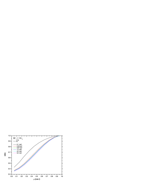
(a) Limb-darkening in the fluid frame at $r=1.6r_{g}$.

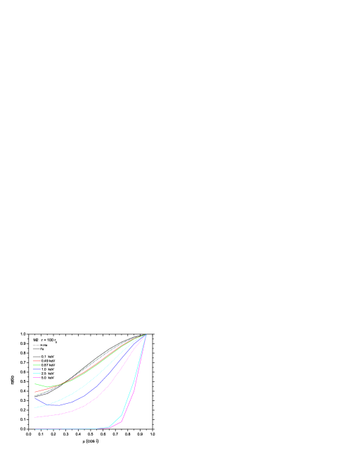
(b) Similar presentation as in part (a) except at $r=100r_{g}$.

Figure 4: Limb-darkening behavior in the local fluid frame for an accretion disk with central BH of $10^{2}~{}M_{\odot}$ and maximum spin. Curves in different colors represent different emission energies. Solid and dotted curves are for the Fe and H-He disks, respectively. Each curve is normalized separately so that in all cases the maximum relative intensity is unity.

For the most part, the chemical composition of the disk doesn’t dramatically affect the angle-dependence of the intensity in the fluid frame no matter which case we are talking about. Roughly speaking, the intensity obeys a linear limb-darkening law in the fluid frame for most energies at all radii. The origin of this linear limb-darkening is very conventional: at larger viewing angles, the apparent photosphere lies nearer the surface, where the temperature is lower. The variation is smooth enough that $T_{\rm apparent}(\mu)$ can be approximated as linear. For energies below the peak of the Planckian (i.e., in the Rayleigh-Jeans regime), $I_{\nu}(0)\propto T_{\rm apparent}$, whence the linear dependence of emergent intensity on $\mu$.

The exception to this rule comes at high energies and large radii. Beyond 1 keV, $T_{\rm apparent}$ continues to be a linear function of $\mu$, but the energies now lie on the Wien side of the Planckian. In that regime, the dependence of intensity on temperature is strongly nonlinear. As the energy increases, this dependence becomes stronger and stronger so that the limb-darkening law becomes steeper and steeper, as seen in Fig. 4(b).

Fig. 5 shows the “limb-darkening” behavior for several specific energies as seen in the observer’s frame. Quotes on this term are appropriate because for much of the interesting energy range the limb, or an oblique angle, may actually be the point of view where the light is brightest. Although low energies do show fairly conventional linear limb-darkening, higher energies ($E\geq 1$ keV) exhibit very different behavior. At these energies, there is relatively little pole-to-limb contrast; indeed, the intensity does not even vary monotonically as a function of viewing angle. As the energy increases, the brightest direction moves from $\mu=0.8$ (at 1 keV) to $\mu=0.6$ (at 2.5 keV) and to $\mu=0.45$ (at 5 keV).

A competition between two opposing effects leads to this unusual result. On the one hand, the emergent intensity in the fluid frame is limb-darkened for the reasons just discussed. On the other hand, because orbital motion is in the plane, relativistic beaming tries to push flux toward the limb. The flux at high energy is generated predominantly in the innermost part of disk, so the importance of relativistic limb-brightening grows as the energy increases. This competition accounts for all the effects described in the previous paragraph.

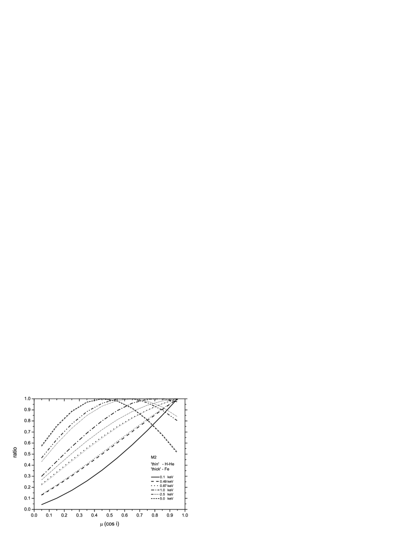
Figure 5: Limb-darkening calculated in the observer’s frame for an accretion disk with central BH of $10^{2}~{}M_{\odot}$ and maximum spin. Thick and thin curves are the Fe and H-He disks, respectively. Curves in different line types represent different emission energies. As in Fig. 4, each curve is normalized so that its maximum is unity.

3.4 Spectra in different metrics

In the previous subsections, we have presented results only from our calculations of a disk in a maximal Kerr metric. Not all black holes spin rapidly, so we have also calculated the spectrum of a disk around a non-spinning $100M_{\odot}$ black hole. The only change in technique was the use of a coarser radius grid, as mentioned in section 2.1. In Fig. 6 we show the results and compare them to the rapidly-spinning case.

Figure 6: Spectra of Fe disks in the observer’s frame with central BH mass $10^{2}~{}M_{\odot}$. The solid, dashed and dotted line types represent different viewing angles, $\mu=0.95,0.55,0.05$, respectively. Schwarzschild and Kerr metrics are represented by the thin and thick curves, respectively.

The biggest contrast between the two cases is that the spectra are “cooler” when the spin is slow. This is a natural outcome of the fact that in the Schwarzschild metric the innermost stable circular orbit—in our model, the inner edge of the disk—is not nearly as deep in the potential as it is in the maximal Kerr metric.

This contrast in the position of the disk inner edge also leads to another contrast between the two cases visible in Fig. 6: slow spin also leads to much weaker Doppler shifting, and therefore much weaker dependence of the observed peak energy on the observer’s viewing angle. The peak energy for the spectrum emitted by a disk around a Schwarzschild black hole changes very little as a function of viewing angle, whereas in the maximal Kerr case, the energy of the peak moves from 0.81 keV to 3.3keV when $\mu$ changes from 0.95 to 0.05.

What does change with viewing angle in the Schwarzschild case is the flux itself. From the pole-on to the edge-on view, the flux falls by about a factor of 15. The corresponding ratio for the Kerr case is only about 1.5. Integrated over solid angle, the observed bolometric luminosities at infinity are 76% and 97% of the assumed $0.1L_{Edd}$ for the Kerr and Schwarzschild cases, respectively; the missing radiation is in photons that either return to the disk or are captured by the black hole (cf. Agol & Krolik 2000 who computed the capture and returning radiation fractions for emission isotropic in the fluid frame).

In addition, when the relativistic Doppler shifts are comparatively weak, remnants of the photoionization features imprinted on the fluid frame spectra survive in the integrated spectrum. When the black hole spins slowly, this is the case at all angles, but when the extreme Kerr metric applies, this is true only for nearly face-on viewing angles.

The form these features take is a “platform” around the peak area. Because it is based on the CVI and OVIII edges, it runs from $\simeq 500$ eV to $\simeq 870$ eV, with these boundaries changed only slightly by angle-dependent Doppler shifts. We stress that the spectral shape in this region is not a classic ionization edge; rather, there are breaks in the spectral slope at these energies and the spectrum in between has relatively little curvature.

3.5 Effects of varying central black hole mass

We have also investigated the effects caused by changing the central mass of the black hole from $10^{2}$ (model M2) to $10^{3}~{}M_{\odot}$ (model M3) in the maximal Kerr metric. The most obvious contrast is trivial: at fixed $L/L_{E}$, the luminosity of the disk around the $1000M_{\odot}$ black hole is ten times as great as that of the disk around the $100M_{\odot}$ black hole.

In many respects the shapes of the two spectra are quite similar. They have similar curvature, and they both have the shelf between two ionization features when viewed face-on (Fig. 7). The principal difference in spectral shape between the two cases is the downward shift in energy of the peak as the central mass increases. The ratio between the M2 and M3 peak energies varies hardly at all as a function of viewing angle, as it is $\simeq 1.6$ at $\mu=0.05$, $\simeq 1.8$ at $\mu=0.55$, and $\simeq 1.7$ at $\mu=0.95$. The reason for the shift, of course, is the well-known scaling law for the central temperature of an accretion disk around a black hole: $T\propto M^{-1/4}(L/L_{E})^{1/4}$. In this case, with a factor of 10 between the two masses, the contrast in central temperature is a factor of 1.8. Angle-dependent Doppler shifts and, to a lesser degree, differential atomic opacity effects, cause the angle-dependent ratio in the peak energy to differ slightly from this ratio.

Figure 7: Spectra of Fe disks with central BH masses $10^{2}~{}M_{\odot}$ and $10^{3}~{}M_{\odot}$ in the extreme Kerr metric. The solid, dashed and dotted line types represent viewing angles $\mu=0.95,0.55,0.05$. The thick and thin curves are for $10^{2}~{}M_{\odot}$ and $10^{3}~{}M_{\odot}$ black holes.

There is also a small change in the photoionization features correlated with the temperature contrast between the two models with different central masses. We note that these features are visible only when the viewing angle is nearly pole-on because these calculations assume rapidly-spinning black holes. The CVI edge is near the spectral peak for the $1000M_{\odot}$ black hole, and its associated spectral break is correspondingly more prominent than the one associated with the OVIII edge. In the hotter disk around the $100M_{\odot}$ black hole, the situation is exactly reversed: The OVIII edge is nearer the peak and creates a sharper spectral break.

4 Discussion

4.1 How do our spectra compare to the MCD model?

As we have remarked earlier, there are two principal physical assumptions on which the MCD model rests: 1) The mean intensity in the fluid frame is a dilute blackbody with a fixed dilution factor, and 2) the angle-dependence of the intensity in that frame follows a single predetermined limb-darkening law that is independent of photon frequency. In this section we will assess the quality of those assumptions.

In Fig. 8, we show the emergent flux in the fluid frame at a number of radii, contrasting our results with those predicted by a dilute blackbody. The dilution factor we use is 1.7, the number chosen by many authors including Gierlinski et al 2001. Without heavy elements, the DBB model is a reasonable approximation to the actual solution (see, Fabian et al 2004), but with a distinct shift of flux from low frequencies to high (Fig. 8(a)). Generally speaking, the DBB model falls a factor of 2 or so below the fluid-frame flux computed in the full atmosphere model at frequencies 10 times below the peak. It agrees reasonably well with the full calculation for frequencies within a factor of 3 above or below the peak at large radii ($r\geq 10r_{g}$), but predicts $\sim 10\%$ too much flux near the peak at small radii. At energies well above the peak, the DBB model predicts too little flux at large radii and too much at small.

These deviations of the DBB from the full calculation are most likely related to the fact (pointed out in § 3.1) that a modified blackbody spectrum is a better approximation to the emergent intensity in the fluid frame than a dilute blackbody. The DBB assumes that the factor multiplying the Planckian is a constant, but $\sqrt{\epsilon_{\nu}}\propto\nu^{-1}$ when the free-free process is the dominant absorptive opacity. Although this frequency-dependence is partially offset by the fact that $T^{*}$ decreases toward lower frequency, there is still a net rise toward low frequencies relative to the constant multiplicative factor of the DBB model.

In addition, smaller deviations can be seen around the peak area, particularly at larger radius, even in the absence of heavy elements. For example, the DBB flux near the spectral peak at $r=20r_{g}$ is 17% too high. We expect that this discrepancy is mostly due to the other place where $f$ appears, where it is used as a “hardening factor” to shift the nominal temperature of the thermal spectrum. Even in a pure H-He atmosphere, because the temperature gradient changes from place to place, just as no single dilution factor works for all radii, neither does any single value of $T^{*}/T_{\rm eff}$.

(a) Pure H-He atmosphere.

(b) Atmosphere with H, He, C, N, O, and Fe.

Figure 8: Emergent flux in the local fluid frame for a series of annuli in an accretion disk around a $10^{2}~{}M_{\odot}$ extreme Kerr black hole. Thick curves are results of our calculations and thin curves represent the DBB model with the same effective temperatures. From top to bottom, the radii corresponding to each pair of curves are: $r/r_{g}$=1.6, 5.0, 10, 20, 50.

When heavy elements are introduced, the quality of fit provided by the DBB model worsens sharply, as shown in Fig. 8(b). For frequencies at the peak or below, the level of agreement is about the same as for the H-He model. However, in the outer rings, where the atomic photoionization features become important (cf. § 3.1), the DBB model predicts far too much flux at frequencies above the peak. It is obvious that this sort of discrepancy in spectral shape is far beyond the ability of a mere change in dilution factor to fix.

We next examine how these local effects carry over into the observed spectrum. In Fig. 9, we present the MCD spectrum (in the definition of Gierlinski et al 2001), and our two full atmosphere spectra (with and without heavy elements) as they would be seen face-on, with the frequency range restricted to the peak region. We see now the MCD spectrum is approximately correct only between 0.6 and 0.8 keV and above 1.6 keV, as it over-predicts the flux from 0.8 to 1.6 keV and falls too steeply toward lower energies below 0.6 keV.

Just as in the fluid frame, the biggest contrasts between the MCD spectrum and the full atmosphere are the result of heavy element opacity. Because the Doppler effect is reduced to a minimum in this face-on view, the heavy element features appear with relatively little smearing, despite the various relativistic effects. The MCD model overpredicts the flux near the peak by about 13%, but more glaringly, drastically misses the shape of the spectrum. Rather than the smoothly curving shape predicted by the MCD between 0.5 and 2 keV, a full atmosphere calculation predicts a spectrum with sharp changes in slope near 490 eV, 560 eV, 810 eV, and 1.5 keV. Gentler changes in spectral slope can be found near 0.4, 1.0, and 1.5 keV. Several of these are clearly associated with photoionization edges of H-like ions: CVI is at 490 eV, OVIII at 871 eV, Fe XIX at 1.538 keV. Others likely represent the end-points of the edge features. Of these, the greatest curvature is associated with the feature that is strongest in the fluid frame, the OVIII edge.

Figure 9: Spectra of accretion disks with different chemical compositions in the observer’s frame at infinity. The central BH mass is $10^{2}~{}M_{\odot}$ and it is in the extreme Kerr metric. Thick curves are results from our calculations (solid curve is the Fe disk and the dashed is H-He); the thin curve shows the MCD model modified by Gierlinski et al 2001. The viewing angle is nearly face-on ($\mu=0.95$). Heavy element features create numerous sharp bends that do not appear when the atmosphere is pure H-He or the MCD approximation is used.

The face-on view is, of course, the angle at which the photoionization features are most prominent. Perhaps a fairer measure of the typical situation is provided by the spectrum at $\mu=0.55$ ($56^{\circ}$ off axis), a direction we find gives the closest approximation to the flux as integrated over solid angle. Fig. 10 shows the spectra predicted by the same three models as in Fig. 9, but for $\mu=0.55$. The contrast between our full atmosphere calculation with heavy elements and the MCD approximation is now weaker, as the features are smeared by the strong Doppler broadening made possible by the Kerr metric. However, even in this case, there is still a significant spectral inflection between 1 and 2 keV.

Figure 10: Spectra of accretion disks with different chemical compositions in the observer’s frame at infinity. The central BH mass is $10^{2}~{}M_{\odot}$ and $a/M=0.998$. Similar legends are used as in Fig. 9. The viewing angle, however, changes to $\mu=0.55$.

Only in the extreme edge-on view does the MCD approximation reproduce reasonably well the spectrum at energies above the peak. When the observer is very close to the orbital plane, the whole spectrum is shifted to much higher energies (the peak moves from $E=0.81$ keV to $E=3.3$ keV, a factor of 4.1 shift), and the atomic fingerprints are totally eliminated by the strong Doppler effect. Even so, the low-frequency deviations (now all frequencies below 1.5 keV) persist unchanged.

4.2 Limb-darkening law of integrated luminosity

We have already discussed (§ 3.3) the angular dependence of the emergent intensity, both in the fluid frame and as seen by a distant observer, at selected energies. Here we explore the angle-dependence of the frequency-integrated intensity as measured in the fluid frame and compare it to approximations in the literature, such as the one used by Gierlinski et al 2001. The results are displayed in Fig. 11, which shows $r=1.6r_{g}$ in the $100M_{\odot}$ extreme Kerr model with heavy elements.

Gierlinski et al. assumed the simple linear approximation $I(\mu)\propto 1+B\mu$ with $B=2.06$ everywhere. On the whole, its description of our full atmosphere calculation is not too bad, both at this radius and at all others. The frequency-integrated limb-darkening is in fact not far from linear, and its slope ($B=2.60\pm 0.01$) is a bit greater than the Gierlinski et al. assumed value.

However, there is still a deviation of as much as 15% between the full calculation and the linear approximation. Virtually all of this deviation can be eliminated by use of a different analytic form with four parameters:

$$I(\mu)\propto A_{2}+\frac{A_{1}-A_{2}}{1+e^{\frac{\mu-\mu_{0}}{\delta\mu}}}$$ (6)

Choosing these as $A_{1}=0.108$, $A_{2}=0.44$, $\mu_{0}=0.48$, and $\delta\mu=0.2$ gives a remarkably good fit to the limb-darkening behavior at all radii for both $100M_{\odot}$ and $1000M_{\odot}$ (Fig. 11).

Figure 11: Comparison of the limb-darkening law calculated by our model to the linear law assumed by Gierlinski et al 2001 in the case of $10^{2}~{}M_{\odot}$. The square data points are calculated from our model at $r=1.6r_{g}$. The solid thick curve is generated using eq. 6 and parameters discussed in the text. The limb-darkening law assumed by Gierlinski et al 2001 is the thin dashed line; our best-fit linear law is the thin solid line.

4.3 Observational Consequences

Although our models are far too few to span the likely range of parameters applicable to IMBHs, their results have a number of implications of immediate interest to the interpretation of observational data.

4.3.1 Temperature–Mass Ambiguities

The first observational implication is one that, at the qualitative level, did not require calculations anywhere near as detailed as ours to make. We merely develop this point in a specific and quantitative way. It is that the mapping between characteristic temperature of an accretion disk spectrum and the mass of the black hole at its center is by no means 1:1. As Figure 6 shows, when the spin parameter is large, the peak energy of the spectrum can increase by as much as a factor of 7 relative to what would be expected from a Schwarzschild black hole. Part of this rise in temperature (for fixed central mass and luminosity) is due to the ability of the disk to extend closer to the black hole in the Kerr than in the Schwarzschild metric; another part is due to Doppler shifting when the viewing angle swings from pole-on to edge-on. Because the expected temperature scaling is $T\propto M^{-1/2}L^{1/4}$, the inferred mass (assuming a Schwarzschild metric) depends on observables as $M_{\rm inferred}\propto T^{-2}L^{1/2}$. The assumption of a non-spinning black hole could thus lead to an underestimate of the central mass by as much as a factor of $\sim 50$.

Conversely, as shown in Figure 7, disks around central masses differing by a factor of 10 can span a largely overlapping range of temperatures if their parent black holes spin rapidly. A larger Doppler shift applied to light from a disk around a more massive black hole can compensate for its intrinsically lower temperature.

Thus, the characteristic energy–black hole mass relation is ambiguous in both directions due to the effects of black hole spin. Observers at different viewing angles can see a wide range of characteristic energies in the light from a single black hole, while a wide range of masses can all produce spectra with the same characteristic energy.

4.3.2 Angle-dependence in Bolometric Luminosity Estimates

Estimating the correct bolometric luminosity is subject to analogous problems. Reference to Figure 6 also shows that the apparent luminosity can vary by more than an order of magnitude due solely to radiation anisotropy. Unlike the temperature shift, this problem is most severe when the black hole rotates slowly if one has sufficiently broad-band spectral data. However, with limited band-pass, the temperature shifts associated with viewing angle changes in the maximal Kerr case can lead to errors in the bolometric luminosity that are at least as large.

4.3.3 Possible Visibility of Atomic Features

As we have stressed, one of our most important new results is the influence of atomic photoionization features, principally the K-edges of CVI and OVIII, on the emergent spectrum. Best seen in the spectra from disks around slowly-spinning black holes at all viewing angles or in the spectra of disks around rapidly-spinning black holes viewed face-on, these features create several sharp breaks in slope near the peak of the spectrum when $M\sim 100$–$1000M_{\odot}$, most prominently near 490 eV and 810 eV. Because these features are due to H-like species, it is possible that photoionization by hard X-rays could reduce their strength; the extent to which that may be so depends on how much of the hard X-ray continuum we see also shines on the annuli principally responsible for these features, $10\leq r/r_{g}\leq 20$ for OVIII, $20\leq r/r_{g}\leq 30$ for CVI, for the parameters considered here. It is possible that the hard X-ray source is sufficiently centrally concentrated or beamed outward as to not greatly affect the feature-producing radii. Detection of (or bounds on) an Fe K$\alpha$ feature in these objects would help constrain the amount and distribution of disk irradiation.

5 Summary and Conclusion

By constructing detailed atmosphere models for the disks around intermediate mass black holes, we have shown that their spectra possess a characteristic signature (almost) unique to the mass range 100–$1000M_{\odot}$: atomic photoionization features near the peak of the thermal spectrum. These are present because the energies of the K-edges in astrophysically abundant medium-$Z$ elements are in the range 0.3–1 keV (depending on ionization state and $Z$), and only in this mass range is the (fluid frame) peak energy in the spectrum of moderately sub-Eddington disks around black holes $\lesssim 1$ kev. Higher mass black holes have lower temperatures, so equivalent features due to H and He can appear in disk spectra for $\sim 10^{6}$–$10^{7}M_{\odot}$ black holes, but are also often subject to Comptonization smearing (Hubeny, Blaes, Agol, &Krolik 2001). Lower mass black holes are so hot at their centers that all the abundant elements but Fe are thoroughly stripped.

A comparison of models with different central masses and different spin parameters shows that there are sizable ambiguities that interfere with linking observed parameters of X-ray sources with the mass of the black hole responsible. It is important for the interpretation of observed spectra that these systematic uncertainties be acknowledged.

Finally, we have made a close comparison of the popular MCD approximation with our more thorough calculations. This comparison is made somewhat multivalent by the numerous variations on this approximation found in the literature (relativistic disk model or simple $T\propto r^{-3/4}$? which limb-darkening law? relativistic transfer function applied?). To serve as our standard of comparison, we have chosen the most careful of the various versions, that of Gierlinski et al 2001. We find that if the accretion fuel came from Population II (or III) sources, the MCD approximation would be fairly good, although there is a potentially observable slope discrepancy at low energies. However, the importance of heavy element photoionization opacity in solar abundance material at the temperatures prevalent in disks around black holes of 100–$1000M_{\odot}$ renders the MCD approximation much less accurate. Similarly, although the linear limb-darkening law chosen by Gierlinski et al 2001 gives a fairly good description of the frequency-integrated angle-dependence of the emergent intensity, it fails in interesting ways when applied to the angle-dependence of the frequency-dependent intensity, particularly for energies $>1$ keV.

References

- Agol (1997) Agol, E. 1997, Ph.D dissertation
- Agol & Krolik (2000) Agol, E., & Krolik, J. H. 2000, ApJ, 528, 161
- Anders & Grevesse (1989) Anders, E., & Grevesse, N. 1989, Geochim. Cosmochim. Acta, 53, 197
- Balbus & Hawley (1998) Balbus, S. A., & Hawley, J. F. 1998, Rev. Mod. Phys., 70, 1
- Begelman (2002) Begelman, M., 2002, ApJ, 568, L97
- Colbert & Miller (2004) Colbert, E. J. M., & Miller, M. C. 2004, (astro-ph/0402677)
- Colbert & Mushotzky (1999) Colbert, E. J. M., & Mushotzky, R. F. 1999, ApJ, 519, 89
- Colbert & Ptak (2002) Colbert, E. J. M., & Ptak, A. F. 2002, ApJS, 143, 25
- Davis et al (2004) Davis, S. W., Blaes, O. M., Hubeny, I., & Turner, N. J. 2004, (astro-ph/0408590)
- Fabbiano & Trinchieri (1987) Fabbiano, G., & Trinchieri, G. 1987, ApJ, 315, 46
- Fabian et al (2004) Fabian, A. C., Ross, R. R., & Miller, J. M. 2004, MNRAS, 355, 359
- Gierlinski et al (2001) Gierlinski, M., Maciolek-Niedzwiecki, A., & Ebisawa, K. 2001, MNRAS, 325, 1253
- Hubeny, Agol, Blaes, &Krolik (2000) Hubeny, I., Agol, E., Blaes, O., & Krolik, J. H. 2000, ApJ, 533, 710
- Hubeny, Blaes, Agol, &Krolik (2001) Hubeny, I., Blaes, O., Agol, E., & Krolik, J. H. 2001, ApJ, 559, 680
- Hubeny, Hubeny (1998) Hubeny, I., & Hubeny, V. 1998, ApJ, 505, 558
- Hubeny, Lanz (1995) Hubeny, I., & Lanz, T. 1995, ApJ, 439, 875
- Kaaret et al (2004) Kaaret, P., Ward, M. J., & Zezas, A., 2004, MNRAS, 351, L83
- King et al (2001) King, A. R., Davies, M. B., Ward, M. J., Fabbiano, G., & Elvis, M. 2001, ApJ, 552, L109
- Krolik (1999) Krolik, J. H. 1999, Active Galactic Nuclei: From the Central Black Hole to the Galactic Environment (Princeton: Princeton University Press)
- Li et al (2004) Li, L. X., Zimmerman, E. R., Narayan, R., McClintock, J. E., 2004, (astro-ph/0411583)
- Lynden-Bell & Pringle (1974) Lynden-Bell, D. & Pringle, J. 1974, MNRAS 168, 603
- Makishima et al (1986) Makishima, K., et al 1986, ApJ, 308, 635
- Makishima et al (2000) Makishima, K., et al 2000, ApJ, 535, 632
- Merloni et al (2000) Merloni, A., Fabian, A. C., Ross, R. R., 2000, MNRAS, 313, 193M
- Mihalas (1978) Mihalas, D. 1978, Stellar Atmospheres (2nd Ed., San Francisco, Freeman)
- Miller et al (2003) Miller, J. M., Fabbiano, G., Miller, M. C., & Fabian, A. C. 2003, ApJ, 585, L37
- Miller et al (2004) Miller, J. M., Fabian, A. C., & Miller, M. C. 2004, ApJ, 607, 931
- Miller & Hamilton (2002) Millis, M. C., Hamilton, D. P. 2002, MNRAS, 330, 232
- Mitsuda et al (1984) Mitsuda, K. et al 1984, PASJ, 36, 741
- Nolan et al (2004) Nolan, L. A., Ponman, T.J., Read, A.M., & Schweizer, F. 2004, (astro-ph/0405557)
- Novikov, & Thorne (1973) Novikov, I. D., & Thorne, K. S. 1973, in Black Holes, eds. C. De Witt& B. De Witt (New York: Gordon and Breach), 343
- Page, & Thorne (1974) Page, D. N., & Thorne, K. S. 1974, ApJ, 191, 499
- Pakull & Mirioni (2003) Pakull, M. W., & Mirioni, L. 2003, RevMexAA (Serie de Conferencias), 15, 197
- Roberts, et al (2004) Roberts, T. P., Warwick, R. S., Ward, M. J., & Goad, M. R. 2004, MNRAS, 349, 1193R
- Ross & Fabian (1996) Ross, R. R., Fabian, A. C. 1996, MNRAS, 281, 637
- Rybicki & Lightman (1979) Rybicki, G. B, & Lightman, A. P. 1979, Radiative Processes in Astrophysics (New York, Wiley)
- Shakura, Sunyaev (1973) Shakura, N. I., Sunyaev, R. A. 1973, A&A, 24, 337
- Shimura & Takahara (1995) Shimura, T., Takahara, F. 1995, ApJ, 445, 780
- Stobbart, et al (2004) Stobbart, A. M., Roberts, T. P., & Warwick, R. S. 2004, MNRAS, 351, 1063S
- Strickland, et al (2001) Strickland, D. K., Colbert, E. J. M., Heckman, T. M., Weaver, K. A., Dahlem, M., & Stevens, I. R. 2001, ApJ, 560, 707
- Swartz, et al (2002) Swartz, D. A., Ghosh, K. K., & Tennant, A. F. 2002, 201st AAS Meeting, #54.13, Bulletin of the American Astronomical Society, Vol. 34, p.1200
- Thorne (1974) Thorne, K.S. 1974, Ap.J. 191, 507