The complete set of ASCA X-ray observations of non-magnetic cataclysmic variables

Abstract

We present the complete set of thirty four ASCA observations of non-magnetic cataclysmic variables. Timing analysis reveals large X-ray flux variations in dwarf novae in outburst (Z Cam, SS Cyg and SU UMa) and orbital modulation in high inclination systems (including OY Car, HT Cas, U Gem, T Leo). We also found episodes of unusually low accretion rate during quiescence (VW Hyi and SS Cyg). Spectral analysis reveals broad temperature distributions in individual systems, with emission weighted to lower temperatures in dwarf novae in outburst. Absorption in excess of interstellar values is required in dwarf novae in outburst, but not in quiescence. We also find evidence for sub-solar abundances and X-ray reflection in the brightest systems.

LS Peg, V426 Oph and EI UMa have X-ray spectra that are distinct from the rest of the sample and all three exhibit candidate X-ray periodicities. We argue that they should be reclassified as intermediate polars.

In the case of V345 Pav we found that the X-ray source had been previously misidentified.

1 Introduction

Cataclysmic variables are close binary stars in which a white dwarf accretes material lost from a Roche-lobe filling late-type companion. Non-magnetic cataclysmic variables are the subset of systems in which the magnetic field of the white dwarf is not sufficiently strong to dominate the dynamics of the accretion flow. In these systems the accreting material forms an accretion disc around the white dwarf (see warnersbook for a review of cataclysmic variables).

The proximity of many cataclysmic variables and the relative faintness of their stellar components makes their accretion discs unusually accessible. Their discs also evolve on accessible timescales of days and weeks, allowing us to make detailed observations of their behaviour. An important subclass of non-magnetic cataclysmic variables are the dwarf novae, so named because of dramatic outbursts in which their accretion discs brighten by a factor of around one hundred. These outbursts are believed to be the result of a thermal-viscous instability in the accretion disc (for a review see lasotareview).

Non-magnetic cataclysmic variables tend to be reasonably bright X-ray sources with luminosities of $10^{30}$–$10^{32}$ erg s^-1 rosatcvs. Observations of eclipsing systems have shown that X-ray emission originates very close to the white dwarf, at least in quiescence htcas,zcha,oycareph,oycarxmmpj. X-rays are probably emitted through shock heating of gas in a narrow boundary layer between the accretion disc and white dwarf where the accreting material gives up its kinetic energy and settles onto the white dwarf surface. X-ray observations of non-magnetic cataclysmic variables are therefore sensitive to the accretion rate through the accretion disc, and to the conditions in the inner accretion disc.

In this paper we present the complete set of ASCA X-ray observations of non-magnetic cataclysmic variables. Previous work on samples of X-ray observations of non-magnetic cataclysmic variables has included observations from HEAO-1  [Cordova, Jensen & Nugent¡1981¿], Einstein [Cordova & Mason¡1984¿, Eracleous, Patterson & Halpern¡1991¿, Eracleous, Halpern & Patterson¡1991¿], EXOSAT  [Mukai & Shiokawa¡1993¿], and ROSAT  [Vrtilek et al.¡1994¿, Van Teeseling & Verbunt¡1994¿, Van Teeseling, Beuermann & Verbunt¡1996¿, Richman¡1996¿, Verbunt et al.¡1997¿]. ASCA  made long observations of cataclysmic variables, with a high effective area across a broad energy range and higher spectral resolution than these previous instruments.

2 Observations

2.1 The ASCA Observatory

The Japanese X-ray observatory ASCA (asca) operated for eight years between 1993 February 20 and 2000 July 14. Its science instruments consisted of four identical grazing-incidence X-ray telescopes (ascaxrt). These telescopes provided sufficient imaging resolution for background rejection and sufficient effective area to detect cataclysmic variables up to 10 keV.

ASCA was notable for being the first X-ray observatory to carry CCD detectors, providing excellent spectral resolution (2 per cent at 5.9 keV). Two of the X-ray telescopes were fitted with identical CCD cameras, the Solid-state Imaging Spectrometers (SIS0 and SIS1). The other two telescopes were fitted with Gas Imaging Spectrometers (GIS2 and GIS3), which had less spectral resolution by a factor $\sim$4, but which were more sensitive above 5 keV and had a much larger field of view. Some of the detections discussed in this paper were serendipitous and made only with the GIS detectors. Both types of detectors were sensitive in the range $\sim$0.6–10 keV.

2.2 Data Reduction

2.2.1 Data screening

Data from ASCA were provided in a relatively raw form and required screening to remove intervals of high background. A standard screening recipe is provided by NASA, but since many of our targets were faint we decided to maximise our coverage by applying our own screening criteria. This involved an iterative process in which the screening parameters for each observation were progressively tightened until we were confident that no high-background intervals remained. As a consequence, different screening parameters were applied to each observation. In a few cases individual high-background intervals were excluded by hand.

The parameters we adjusted between observations were: the maximum allowed telescope deviation from the source position (in the range 0.01–0.02^∘), the minimum allowed angle between the spacecraft pointing and the limb of the Earth (5–18^∘), and the minimum allowed angle between the spacecraft pointing and the sunlit limb of the Earth (for SIS only; 5–35^∘). By selecting different values of these parameters for each observation we were able to rescue many hours of coverage of sources which would otherwise have been lost due to minor excursions across the standard screening limits.

For all the observations we also applied a limit to the background monitor count rate of RBM_CONT$<250$ (compared with RBM_CONT$<100$ in the standard screening). We did not screen on cut-off rigidity (COR). All other parameters were held at the standard screening values.

Table 1: Log of ASCA observations of non-magnetic cataclysmic variables. Types are taken from ritter98 and are defined as follows: DN=dwarf nova, SU=SU UMa subtype, UG=U Gem subtype, ZC=Z Cam subtype, NL=nova-like, Na=fast decline nova, AC=AM CVn star consisting of two He white dwarfs, SH=optical superhumps have been observed, UX=UX UMa subtype (permanent outburst), VY=VY Scl subtype (anti-dwarf nova). The optical state refers to the outburst state of the disc during the ASCA observation, as estimated from AAVSO online light curves, where OB=outburst, T=transition, Q=quiescence, and HS=high state for the nova-like variables. Information on the optical state is not available for all systems. In the count rate column, $<$ indicates a non-detection. The GIS2 hardness are the ratio of counts above and below 2.3 keV.
References to previous publications of these data are (numbered) as follows: 1) Mauche02; 2) baskill01; 3) htcas; 4) ascasscyg; 5) do97; 6) ugemszkody; 7) tleoasca; 8) wzsgeasca.
Distance references (letters) are as follows: a) hippdist, b) thorstensendistances; c) Harrison00; d) Harrison03; e) berriman85; f) patterson84; g) crboo01; h) oycarbruch96; i) wood95; j) v436cen; k) sproats; l) vwhyidist; m) warner87; n) v345pav; p) ktperdist; q) cppupdist.
Inclination references (Greek letters) are as follows: $\alpha$) v603aql2000; $\beta$) shaftersthesis; $\gamma$) ritter98; $\delta$) crboo01; $\varepsilon$) oycar89; $\zeta$) htcasinc; $\eta$) wwcet4; $\theta$) alcom98; $\iota$) thesis; $\kappa$) gpcom99; $\lambda$) 22cvs; $\mu$) ugeminc; $\nu$) vwhyiinc; $\xi$) tleoinc; $\pi$) bklyninc; $\rho$) v426oph88; $\sigma$) v345pav; $\tau$) lspeginc; $\upsilon$) cppupinc; $\phi$) wzsgeinc; $\chi$) suumainc; $\psi$) cuvel; $\omega$) ixvel.

		Orbital				Obs.	Exp.	Count rate		Hardness
		Period		Observation	Optical	length	Time	[s-1]		ratio	Distance
Target	Type	(hrs)	Inclination	Date	State	[ks]	[ks]	SIS0	GIS2	GIS2	[pc]	References
V603 Aql	Na SH	3.314	13${}^{o}\pm$2o	1996 Oct 8	HS	115	45	0.81	0.44	0.67	237$\pm^{380}_{\phantom{3}90}$	a,$\alpha$
TT Ari	NL VY	3.301	-	1994 Jan 20	HS	50	20	0.38	0.23	0.69	$>$180	1,e
KR Aur	NL VY	3.907	38${}^{o}\pm$10o	1996 Mar 6	HS	41	22	0.07	0.03	0.58	180	1,f,$\beta,\gamma$
CR Boo	NL AC	0.409	30${}^{o}\pm$5o	1999 Jan 6	HS?	95	43	0.03	0.02	0.35	450$\pm$50	g,$\delta$
Z Cam	DN ZC	6.956	57${}^{o}\pm$11o	1995 Mar 7	OB	353	80	0.04	0.02	0.59	163${}^{+68}_{-38}$	2,b,$\beta,\gamma$
				1997 Apr 12	T	36	17	0.39	0.26	1.18
OY Car	DN SU	1.515	83.3${}^{o}\pm$0.2o	2000 Jan 28	Q	150	42	0.04	0.03	1.03	86$\pm$4	h,$\epsilon$
HT Cas	DN SU	1.768	81${}^{o}\pm$1o	1994 Sep 6	Q	82	34	0.07	0.05	1.00	165$\pm$16	3,i,$\zeta$
V436 Cen	DN SU	1.500	65${}^{o}\pm$5o	1997 Jun 19	Q	66	24	0.44	0.27	0.78	263	j,$\gamma$
WW Cet	DN	4.219	54${}^{o}\pm$4o	1996 Dec 24	Q	41	24	0.44	0.25	0.59	121-171	k,$\eta,\gamma$
AL Com$\dagger*$	DN SU	1.360	20o-40o	1997 Jun 22	?	101	42	-	$<$0.005	-	187-264	k,$\theta$
GO Com$\dagger$	DN SU	1.579	-	1996 Jan 8	?	55	23	-	0.01	0.95	361-510	k
GP Com	NL AC	0.775	49o-70o	1994 Jul 6	?	41	7	0.13	0.07	0.46	68${}^{+7}_{-6}$	b,$\iota,\kappa$
				1994 Jun 30	?	93	27	0.20	0.09	0.52
EY Cyg$\dagger$	DN UG	5.244	$<$60o	1999 Oct 23	Q	84	31	-	0.02	0.89	-	$\lambda$
SS Cyg	DN UG	6.603	37${}^{o}\pm$5o	1993 May 26	OB	78	31	1.46	0.67	0.53	166$\pm 13$	4,5,c,$\beta,\gamma$
				1995 Nov 27	Q	46	23	0.53	0.30	0.68
U Gem	DN UG	4.246	69.7${}^{o}\pm$0.7o	1994 Oct 20	Q	71	34	0.35	0.21	0.73	96$\pm^{5}_{4}$	6,c,$\nu$
				1994 Nov 11	Q	59	29	0.38	0.22	0.78
VW Hyi	DN SU	1.783	60${}^{o}\pm$10o	1993 Nov 8	Q	37	14	0.12	0.08	0.44	82$\pm$5	l,$\mu$
				1995 Mar 6	Q	27	6	0.03	0.02	0.51
T Leo	DN SU	1.412	28o-65o	1998 Dec 13	Q	72	31	0.30	0.17	0.51	101${}^{+13}_{-11}$	7,b,$\xi$
BK Lyn$\dagger*$	NL SH	1.800	19o-44o	1996 Nov 13	?	44	23	-	$<$0.004	-	$>$114	k,$\pi$
V426 Oph	DN ZC	6.847	59${}^{o}\pm$6o	1994 Sep 18	Q	41	17	0.40	0.36	2.05	100	m,$\rho$
V345 Pav$\dagger*$	NL UX	4.754	$>$70o	1994 Sep 23	?	48	25	-	$<$0.10	-	630$\pm$100	n,$\sigma$
LS Peg	NL DQ?	4.19	$\approx$30o	1998 Nov 23	?	76	28	0.03	0.02	1.97	-	7,$\tau$
RU Peg	DN UG	8.990	33${}^{o}\pm$5o	1994 Jun 27	OB	43	18	0.08	0.06	0.50	287$\pm^{23}_{20}$	d,$\beta,\gamma$
KT Per$\dagger*$	DN ZC	3.905	-	1998 Jan 24	OB	9	7	-	$<$0.005	-	245$\pm$100	p
CP Pup$\dagger$	Na SH?	1.474	30${}^{o}\pm$5o	1998 Nov 06	?	121	48	-	0.02	0.90	$>$184	q,$\upsilon$
WZ Sge	DN SU	1.361	75${}^{o}\pm$2o	1996 May 15	Q	82	38	0.11	0.08	0.62	43.5$\pm 0.3$	8,d,$\phi$
EI UMa	DN UG	6.434	-	1995 Apr 14	?	41	23	0.52	0.33	1.17	-
SU UMa	DN SU	1.832	44${}^{o}\pm$8o	1997 Apr 12	OB	47	21	0.08	0.05	0.54	260${}^{+190}_{-90}$	b,$\chi$
CU Vel$\dagger$	DN SU	1.884	59${}^{o}\pm$6o	1994 May 31	Q	236	94	-	0.009	0.48	-	$\psi$
IX Vel	NL UX	4.654	60${}^{o}\pm$5o	1995 Oct 29	HS	60	21	0.22	0.12	0.5	96$\pm^{10}_{\phantom{0}8}$	a,$\omega$

$\dagger$ serendipitous observation (GIS only)
$*$ Non-detections

2.2.2 Time series extraction

Lightcurves were extracted without energy cuts from all four detectors for all of our observations. We also extracted hardness-ratio time series from the GIS detectors, using energy ranges of 0.6–2.3 keV and 2.3–10 keV. We used source extraction circles with radii depending on brightness of the source in the range 6–19 arcmin in the SIS instruments and 4–11 arcmin in the GIS instruments. Background rates were estimated using most of the remainder of the detector. Light curves were binned into 16 s bins for power spectral analysis. The light curves plotted in this paper have been rebinned into an integer number of bins per observing interval, with bin sizes in the range 0.25–4 ks (depending on count rate).

2.2.3 Spectral extraction

X-ray spectra were extracted for all four instruments using the same extraction regions as for the time series. Spectra from the two SIS instruments were combined, as were spectra from the two GIS instruments. The resulting spectra were binned to a minimum of 20 counts per bin, so that the $\chi^{2}$ statistic could be used to test the goodness-of-fit of our models [Yaqoob¡1998¿]. During the later years of the mission the CCD detectors became gradually degraded, and the low-energy response became increasingly uncertain. We therefore applied a minimum energy cut to the SIS spectra that increased from 0.6 keV to 0.8 keV during the course of the mission. We also applied a more extreme cut at 1.2 keV in the case of T Leo, where there is an apparent inconsistency in the calibration of the SIS and GIS spectra. Response matrices were generated for each SIS spectrum, since the spectral resolution of the SIS instruments degraded substantially during the course of the mission. The standard response matrix was used for all GIS observations (v1.4).

3 The sample

3.1 Selection criteria and count rates

In order to find all ASCA observations of cataclysmic variables we cross-correlated the ASCA observations catalogue held by the Leicester Database and Archive Service (LEDAS) with the Ritter & Kolb catalogue [Ritter & Kolb¡1998¿]. Correlations were accepted within a 30 arcmin search radius.

In total we found 85 observations of cataclysmic variables. Of these, 46 observations were of magnetic cataclysmic variables (17 observations of polars and 29 of intermediate polars) and 5 observations were of super-soft sources. These observations have been omitted from our sample. This leaves 23 observations of dwarf novae, of which 4 are repeat observations of a source, and 11 observations of novae and nova-likes, one of which is a repeat observation. A log of the ASCA observations of non-magnetic cataclysmic variables is presented in Table 1 together with system parameters, the optical state at the time of the observation (if available) the mean SIS0 and GIS2 count rates (without energy cuts, and without corrections for vignetting), and the GIS2 hardness ratio (the ratio of counts above and below 2.3 keV). We note that 25 out of the 29 non-magnetic cataclysmic variables were detected, including four serendipitous GIS-only detections. The mean GIS2 count rates are plotted as a histogram in Fig. 1. It can be seen that SS Cyg has the highest observed flux of any of the non-magnetic cataclysmic variables, even though it was observed during outburst when the X-ray count rate is expected to be suppressed by a factor of $\sim$5 (Wheatley03). The fainter observation of SS Cyg was made in an exceptionally faint quiescent state (see Sect. 4.1.1). For each observation, the optical state was determined through inspection of AAVSO visual light curves (where available) and these are summarised in Table 2.

Table 2: Summary of the optical states of non-magnetic cataclysmic variables observed with ASCA.

		No.  of	No.  of
Type	Optical state	targets	obs.
Dwarf novae	all states	19	23
	outburst	5	6
	quiescence	12	14
	unknown	3	3
Novae & nova-likes	all states	10	11
	high-state	5	5
	unknown	5	6

Figure 1: Count rates of the non-magnetic cataclysmic variables observed with the ASCA GIS2 instrument. Where multiple observations have been made, they have been plotted separately.

3.2 Hardness ratios

Figure 2: Histogram of the ASCA  GIS2 hardness ratio for all our observations.

Figure 3: Plot of the GIS2 hardness ratios by system class and outburst state (if known). The crosses indicate AM CVn systems. The two systems with extreme hardness in our sample, V426 Oph and LS Peg, are indicated with circles.

Figure 2 shows the distribution of ASCA  GIS hardness ratios. The systems LS Peg and V426 Oph stand out with exceptionally hard X-ray spectra. We discuss these systems in Sect. 7.4 and argue that they should be re-classified as intermediate polars. The hardness ratios are also plotted by type and optical state in Fig. 3. It can be seen that all dwarf novae observed in outburst have relatively soft X-ray spectra. Our spectral analysis of Sect. 5 shows that this is due to an increased contribution by cool gas. Dwarf novae in quiescence exhibit a much wider range of hardness. Nova-likes appear to be intermediate between the two. In order to make quantitative comparisons between the distributions, we have carried out Kolmogorov-Smirnov tests (excluding LS Peg and V426 Oph). This shows that the nova-like hardness distribution is most similar to the outburst hardness distribution, with a KS probability of 0.79. There is less similarity between the outburst and quiescent hardness distributions (KS probability of 0.25), or the quiescent and nova-like hardness distributions (KS probability of 0.45).

3.3 X-ray identification of V345 Pavonis

V345 Pav (EC 19314-5915) is an optically bright eclipsing cataclysmic variable discovered in the Edinburgh-Cape blue object survey [Buckley et al.¡1992¿]. Buckley et al.  suggest that V345 Pav is the optical counterpart of the HEAO-1  X-ray source 1H1930-589. However, the ASCA  GIS image shows that the HEAO-1  source actually lies 9 arcmin from the position of V345 Pav. The brighter X-ray source is coincident with the bright star CD-59 7229 (V=10.5). This star has a B-V colour of +1.1 indicating that it may be a late-type coronally-active star.

4 Timing Analysis

We analysed the temporal behaviour of our sample of ASCA observations beginning at the longest available timescales and moving progressively to shorter timescales. The longest available timescales are years, due to repeat observations of individual systems. The shortest timescales are set by the time-resolution of our individual observations, usually 16 s.

4.1 Repeat observations

Four of the systems in our sample were observed more than once with ASCA, allowing us to detect variations over long timescales.

Z Cam was observed with ASCA  both in outburst and during a transition to outburst. During the transition the ASCA  count rate dropped rapidly as the X-rays were suppressed. During outburst the ASCA count rate remained low. These observations have been discussed in detail by baskill01. U Gem was observed twice in quiescence, with a similar count rate in both cases. These observations were discussed by ugemszkody. The repeat observations of SS Cyg and VW Hyi have not been presented elsewhere, and so we describe them here in more detail.

4.1.1 SS Cygni

Figure 4: Optical lightcurve (top), X-ray lightcurve (middle) and X-ray hardness ratio (bottom) of SS Cyg during the two ASCA observations. The X-ray count rate is found to be unusually low in quiescence.

SS Cyg was observed twice with ASCA, with two and a half years between the observations. It was the only dwarf nova to be observed in both outburst and quiescence with ASCA. The outburst data have been published previously by ascasscyg and do97 but the quiescent observation has not been presented elsewhere.

The ASCA lightcurves of SS Cyg are shown in Fig. 4. Remarkably the count rate was higher in outburst than in quiescence. This is in contrast to all previous X-ray observations of SS Cyg Ricketts79,Jones92,Wheatley03.

Comparison of our ASCA  fluxes with previous observations of SS Cyg (assuming our fitted spectra of Sect. 5) shows that the outburst brightness was normal, and that the quiescent brightness was unusually faint. For instance, Wheatley03 found 3–20 keV fluxes of 1–4$\times 10^{-11}\rm\,erg\,s^{-1}\,cm^{-2}$ in outburst and 10–16$\times 10^{-11}\rm\,erg\,s^{-1}\,cm^{-2}$ in quiescence. Integrating our best fitting spectral models over this range yields ASCA fluxes of 3$\times 10^{-11}\rm\,erg\,s^{-1}\,cm^{-2}$ and 2$\times 10^{-11}\rm\,erg\,s^{-1}\,cm^{-2}$ respectively. None of the previous X-ray observations of SS Cyg show such a low flux in quiescence.

Figure 4 also shows the hardness ratio of SS Cyg during these two observations. It can be seen that the hardness ratio was constant in both observations, but that the outburst observation was softer than the quiescent observation. This behaviour is consistent with that seen in previous observations of this object Wheatley03 and of other non-magnetic cataclysmic variables (Fig. 3).

4.1.2 VW Hydri

Figure 5: Optical lightcurve (top), X-ray lightcurve (middle) and X-ray hardness ratio (bottom) of VW Hyi during the two ASCA observations. The X-ray count rate differs by almost an order of magnitude, even though both observations were made during quiescent intervals.

Table 3: Comparison of X-ray fluxes of VW Hyi in quiescence. All fluxes are in units of $10^{-12}\,\rm erg\,s^{-1}\,cm^{-2}$.

	Bandpass		ASCA Fluxes
Inst.	[keV]	Flux	Obs. 1	Obs. 2
EXOSAT	0.04-16	15a	6.1	1.6
ROSAT+Ginga	0.04-10	21b	6.8	1.9
BeppoSAX	0.14-10	15c	6.5	1.8
XMM-Newton	0.24-12	6d	6.2	1.8

^a vwhyiexosat ^b wheatley96a
^c vwhyibepposax ^d pandel03

VW Hyi was observed twice with ASCA, but neither observation has been published. We present both ASCA  lightcurves of VW Hyi in Fig. 5. Both observations were made during quiescence, but there is a four-fold difference in the X-ray count rates. This behaviour demonstrates the value of X-ray observations of such systems. While the optical emission is sensitive to the global state of the accretion disc, it is clear that there must also be activity in the inner disc that does not correlate with the optical emission. The hardness ratios in the two observations are consistent ($0.52\pm 0.12$ in the earlier observation, $0.66\pm 0.31$ in the later), showing that the difference between the two observations was probably due to a changing accretion rate.

In Table 3 we compare our observed ASCA fluxes with previous X-ray observations. In each case we calculate ASCA fluxes in the same energy range as the published fluxes using our best-fitting spectral model of Sect. 5. VW Hyi was fainter during our first ASCA observation than during most previous observations, but the measured flux is consistent with that seen by pandel03 with XMM-Newton. The flux during our second ASCA observation is much fainter than any of the previous X-ray observations of VW Hyi.

Figure 5 shows that the bright ASCA observation was made in a short period of quiescence between a superoutburst and a normal outburst, whereas the faint observation was made in the middle of a longer quiescent interval. One might imagine that the difference between these observations is related to their relative proximity to outbursts. However, both the XMM-Newton and ROSAT/Ginga observations were also made in the middle of quiescent intervals. It is clear that there is no simple relationship between X-ray flux and inter-outburst phase.

4.2 Long-timescale variations within observations

In order to search for overall brightness variations on the timescale of our observations we carried out a least-squares linear fit to all our SIS0 lightcurves. Our sensitivity is not the same in each case, due to the range of observation duration and source brightness, but we do detect overall brightness variations in four cases.

The best fit gradient for each observation is plotted in Fig. 6. Seven observations have well constrained gradients at the 3-$\sigma$ level. However, three of these exhibit fractional variations that are less than one per cent per day, and we regard these as essentially constant. The remaining four systems all have gradients greater than thirty per cent per day, and these systems are listed in Table 4. All four are dwarf novae, three of which were in outburst during the observation. With three of the the six outburst observations showing an overall trend, and only one of the fourteen quiescent observations, it is clear that the outburst state is most closely associated with large scale X-ray flux variations.

Figure 6: Best fit gradients for all our SIS0 lightcurves versus the significance of their deviation from constancy (in $\sigma$). Gradients are normalised by count rate, so represent the fractional variation per day.

Table 4: Observations for which a gradient was detected in the SIS0 lightcurve.

Target	State	Duration	Countsa	Gradientb	Sig .
Z Cam	T	36 ks	0.39 s-1	$-3.0\pm$0.3	$9.4\sigma$
SS Cyg	OB	78 ks	1.46 s-1	$-0.3\pm$0.1	$4.3\sigma$
SU UMa	OB	47 ks	0.08 s-1	$0.7\pm$0.2	$4.1\sigma$
WW Cet	Q	41 ks	0.44 s-1	$-0.8\pm$0.2	$3.7\sigma$

^a SIS0 count rate.
^b Fractional variation per day.

The second observation of Z Cam was made during a transition to outburst and showed a dramatic decrease in the ASCA count rate (see also baskill01). This is normal behaviour for dwarf novae. The observation of SS Cyg, made towards the end of an outburst, also shows a decreasing count rate (Fig. 4), although in this case the variation does not appear to be part of the outburst to quiescence transition. SU UMa was observed to be brightening during the second half of the outburst, and its lightcurve is plotted in Fig. 7. The only overall trend detected in a quiescent dwarf nova was in WW Cet, which faded during its 13 h observation. The ASCA  lightcurve of WW Cet is shown in Fig. 8. The observation was made eight days before an outburst. WW Cet has a well defined outburst recurrence time of around sixty days.

Figure 7: Optical lightcurve (top), X-ray lightcurve (middle) and X-ray hardness ratio of SU UMa during the ASCA observation.

Figure 8: Optical lightcurve (top), X-ray lightcurve (middle) and X-ray hardness ratio of WW Cet during the ASCA observation. This is the only case in which an overall flux variation was detected in a dwarf nova in quiescence.

Figure 9 shows the GIS hardness ratio versus count rates for all four systems. In Z Cam the hardness ratio increased during the early part of the X-ray suppression, and in SS Cyg the hardness ratio dropped slightly during the decline, but in general the spectra remained stable during these flux variations.

Figure 9: ASCA GIS hardness as a function of count rate for the four observations in which overall flux variations are observed.

4.3 Orbital modulation

We have calculated power spectra for all our ASCA  lightcurves of non-magnetic cataclysmic variables. We used the Lomb-Scargle algorithm, as implemented by powerspec, but with a slight modification to the normalisation (such that the power spectrum is normalised by expected variance rather than measured variance, which can be dominated by signal). Some of these power spectra are dominated by red noise at low frequencies, and this limited our ability to search for low frequency periodic modulations (see Sect. 4.4). However, since we know a priori the orbital period of each of our systems, we circumvented the problem of red noise by searching our power spectra for peaks centred precisely on the known orbital periods. Of course, this approach does not entirely remove the possibility of contamination by red noise.

Inspecting the power spectra of our thirty light curves we found peaks centred on the orbital period in seven cases. These were observations of OY Car (27.5 cycles covered), HT Cas (12.9 cycles), V436 Cen (12.2 cycles), T Leo (14.2 cycles), V426 Oph (1.7 cycles), EI UMa (1.8 cycles) and both observations of U Gem (4.6 & 3.9 cycles). All are dwarf novae observed in the quiescent state, with the exception of EI UMa for which optical observations were not available. The observations of V426 Oph and EI UMa were not sufficiently long to be sure that these modulations were periodic, but these observations nevertheless do exhibit power close to the known orbital period. The power spectrum of V426 Oph is discussed further in Sect. 4.4.2.

It is striking that this set includes three of the four systems with the highest known inclination angles: OY Car, HT Cas and U Gem, with inclinations of 83.3$\pm$0.2, 81$\pm$1 and 69.7$\pm$0.7^∘respectively [Wood et al.¡1989¿, Horne, Wood & Stiening¡1991¿, Zhang & Robinson¡1987¿]. WZ Sge is the only system in our sample known to have a correspondingly high inclination but which did not exhibit an orbital modulation. Of the remaining systems V436 Cen and V426 Oph may also have relatively high inclinations of 65$\pm$5^∘and 59$\pm$6^∘respectively [Ritter & Kolb¡1998¿, Hessman¡1988¿]. None of the systems in this ASCA sample with suspected orbital modulation are known to have an inclination angle less than 60^∘.

Figure 10: The ASCA SIS0 lightcurves and hardness ratios of four of the seven systems for which we find evidence of an orbital modulation. From left to right: OY Car, HT Cas, V436 Cen, T Leo.

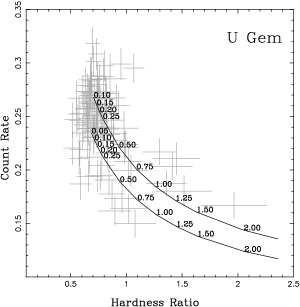
Figure 11: Top: the U Gem lightcurves and hardness ratios from the two observations folded on the orbital period. Bottom: count rates plotted against hardness for both observations. The solid curves represent the relationships expected for the best fitting spectral models of Sect. 5.3 and a range of photo-electric absorption cross-sections (labels are in units of 10²²cm^-2).

The folded GIS1+2 lightcurves and hardness ratios for OY Car, HT Cas, V436 Cen and T Leo are presented in Fig. 10. OY Car and HT Cas are eclipsing systems, and X-ray eclipses are apparent in both folded lightcurves (see also htcas,oycareph,oycarxmmpj). Both systems also show orbital modulation in addition to the eclipses. In the case of OY Car this is anti-correlated with the hardness ratio, suggesting an origin in photo-electric absorption. A similar anti-correlation is also found in lightcurves and hardness ratios of the two observations of U Gem (Fig. 11, and ugemszkody). In Fig. 11 we also plot count rate against hardness ratio and overlay lines of varying absorption column density for the best fit emission spectrum of Sect. 5.3. It can be seen that the variations are broadly consistent with photo-electric absorption. We note that the orbital absorption dips were originally discovered in U Gem by mason88 during an outburst. The ASCA observations are the first in which the absorption dips were detected in quiescence [Szkody et al.¡1996¿]. Mauche03 have modeled Chandra grating spectra of the dips in U Gem and found an acceptable fit with a partial-covering absorber.

In other systems we find that the orbital modulation was not anti-correlated with hardness. The best example is T Leo (Fig. 10 and tleoasca) but the anti-correlation with hardness is also missing in HT Cas and V436 Cen. In V426 Oph and EI UMa the orbital phase coverage was too poor to draw firm conclusions. Orbital X-ray modulation has not been previously claimed in V436 Cen, V426 Oph, or EI UMa.

4.4 Short timescale modulations

The discovery of periodic X-ray modulation (other than the orbital period) is the defining characteristic of intermediate polars. We therefore do not expect to find such periodicities in our sample of non-magnetic cataclysmic variables. Nevertheless, our large set of relatively high signal-to-noise lightcurves may be expected to contain features previously missed with less sensitive instruments. We are encouraged by the detection of a 37 min period in OY Car with XMM-Newton [Ramsay et al.¡2001¿].

The search for periodic modulations in our power spectra was complicated by the presence of red noise that often dominates the low frequencies. At higher frequencies the power spectra are dominated by white noise, and we could apply the standard tests for significance of peaks in the power spectrum [Press & Rybicki¡1989¿].

An inspection of the power spectra of our thirty light curves revealed four candidate periodicities. In each case we required that the peak satisfied the significance test used by powerspeceinstein for Einstein data, and also that it be well separated from obvious red noise peaks. We found candidate periodicities in the power spectra of WW Cet, V426 Oph, LS Peg, and EI UMa. The SIS0 power spectra are plotted in Figs. 12, 13, 14 & 15, and the folded SIS0 lightcurves are presented in Fig. 16.

4.4.1 WW Cet

Significant power was detected at a period of 9.85$\pm 0.05$ min in the SIS0 power spectrum of WW Cet (see Fig. 12). Fitting a sinesoidal function to the folded SIS0 lightcurve we found an amplitude of 11$\pm$1 per cent (where amplitude is the half amplitude of the sine curve divided by the mean). The folded SIS0 lightcurve and best-fit sine function are presented in Fig. 16.

The same peak was seen in the power spectrum of the GIS2 lightcurve, and weakly in the power spectrum of the SIS1 lightcurve, but it was not seen in the GIS3 lightcurve. This difference in the four instruments is due to vignetting resulting from misalignment of the ASCA telescopes. For targeted observations the count rates were highest in the SIS0 and GIS2 instruments and lowest in the SIS1 and GIS3 instruments. Folding on the SIS0 period we found the GIS3 lightcurve to be consistent with our sine fit to the SIS0 lightcurve. We note, however, that the power spectrum of WW Cet contains red noise that dominates at frequencies below 0.001 Hz. Without a thorough understanding of the form of this noise it is difficult to assess whether the detected peak represents a truly period modulation.

Figure 12: SIS0 power spectrum of the ASCA  observation of WW Cet. The horizontal dotted lines indicate the 95 and 99 per confidence limits for detection of significant power above white noise. The labelled peak may represent a true periodicity, but it could instead be a feature of the red noise spectrum.

4.4.2 V426 Oph

At first sight the power spectrum of V426 Oph looks like it is dominated by red noise (Fig. 13). However, closer inspection reveals that several of the peaks are separated by precisely the orbital frequency of the ASCA satellite. Since our lightcurves have gaps on the ASCA orbital period (96 min) we can expect to see power at beat frequencies between real periods and the sampling period. In the power spectrum of Fig. 13 it can be seen that there is power at the orbital frequency of V426 Oph, and that two of the other low frequency peaks can be associated with the beats between this orbital frequency and the ASCA sampling frequency. Also, if we assume the peak at 29.2$\pm$0.9 min represents a real modulation then the two peaks either side of it can also be interpreted as sampling aliases.

We conclude that the X-ray emission of V426 Oph is modulated on a period of 29.2$\pm$0.9 min, with excess power suggestive of orbital modulation. Fitting the SIS0 lightcurve folded at 29.2 min yielded an amplitude of 20$\pm$1 per cent. The folded SIS0 lightcurve and best-fit sine function are presented in Fig. 16. In Sect. 7.4 we argue that V426 Oph should be reclassified as an intermediate polar based independently on its exceptionally hard X-ray spectrum.

V426 Oph has previously been claimed to be an intermediate polar by v426ophip but this evidence was later refuted by v426ophip?. v426ophginga found evidence for a 28 min modulation in the GINGA lightcurve, and it seems likely that this is the same modulation as detected in the ASCA lightcurve. We note that v426ophginga believed the 28 min modulation was not strictly periodic.

Figure 13: SIS0 power spectrum of the ASCA  observation of V426 Oph. The horizontal dotted line indicates the 99 per confidence limits for detection of significant power above white noise. Proposed real periodic modulations are labelled, together with probable sampling aliases separated by the ASCA orbital frequency.

4.4.3 LS Peg

Significant power at a period of 30.9$\pm$0.3 min was detected in the SIS0, GIS2 and GIS3 power spectra of LS Peg (see Fig. 14). The power spectra appear to be relatively free from red noise. Fitting the folded SIS0 lightcurve with a sine function yielded an amplitude of 32$\pm$5 per cent. The folded SIS0 lightcurve and best-fit sine function are presented in Fig. 16. The folded SIS1 lightcurve is consistent with this amplitude.

lspegip report a detection of a period at 29.6$\pm$1.8 min in the circular polarisation of LS Peg. The coincidence of these detected periods leads us to believe that the modulation detected in the ASCA lightcurve is truly periodic, and that the modulation in X-rays and circular polarisation have a common physical origin.

In Sect. 7.4 we argue that the X-ray spectrum of LS Peg is much more like that of an intermediate polar than a non-magnetic cataclysmic variable. The detection of periodic modulation also supports the reclassification of LS Peg as an intermediate polar.

Figure 14: SIS0 power spectrum of the ASCA  observation of LS Peg. The horizontal dotted lines indicate the 95 and 99 per cent confidence limits for the detection of significant power above white noise.

4.4.4 EI UMa

Significant power was detected in the SIS0 power spectrum of EI UMa at a period of 12.36$\pm$0.09 min (see Fig. 15). Fitting a sine function to the folded SIS0 lightcurve we found an amplitude of 8$\pm$1 per cent. The folded SIS0 lightcurve and best-fit sine function are presented in Fig. 16.

This period was seen only in the SIS0 lightcurve and not in the other three instruments. This is probably because the SIS0 count rate is a factor 1.3–3.3 higher than the other instruments. The folded lightcurves of all three are consistent with our fit to the folded SIS0 lightcurve.

This is the first detection of a non-orbital period from this system. In Sect. 7.4 we argue that our fits to the ASCA  spectra of EI UMa require it to be classified, with V426 Oph and LS Peg, as an intermediate polar. The discovery of this period provides supporting evidence for this interpretation.

Figure 15: SIS0 power spectrum of the ASCA  observation of EI UMa. The horizontal dotted lines indicate the 95 and 99 per cent confidence limits for the detection of significant power above white noise.

Figure 16: The ASCA SIS0 folded lightcurves of the four candidate periods from Sect. 4.4. The solid curves represent the sine function fits used to measure pulsation amplitudes. From left to right: WW Cet, V426 Oph, LS Peg and EI UMa. In the case of WW Cet, the observed modulation may merely be a feature of the red noise spectrum.

4.5 ASCA power spectrum of V603 Aql

The ASCA  lightcurve of V603 Aql is of high quality and is of particular interest because evidence of periodic modulations have been found in a previous X-ray observation [Udalski & Schwarzenberg-Czerny¡1989¿]. V603 Aql is also notable for exhibiting both positive and negative superhumps in its optical lightcurves [Patterson et al.¡1997¿].

Udalski89 claim the detection of a 63 min period in the Einstein lightcurve of V603 Aql. powerspeceinstein analyse the same data and agree that there may be a periodic modulation at 63 min or the first harmonic of that period at 31$\pm$2 min, but conclude that further observations are required to establish the stability of this possible modulation. Modulations at similar periods may also be present in the optical lightcurves of V603 Aql [Udalski & Schwarzenberg-Czerny¡1989¿, Patterson et al.¡1997¿]. However, a recent study using ROSAT data found no evidence for an X-ray periodicity [Borczyk, Schwarzenberg-Czerny & Szkody¡2003¿].

We plot the ASCA  SIS0 power spectrum of V603 Aql in Fig. 17. It can be seen that there are prominent peaks close to the orbital period and also close to the 31 min and 63 min periods previously claimed in X-rays. There are, however, several other prominent peaks, and it is clear that there is significant power over a wide range of frequencies. We conclude that the ASCA lightcurves of V603 Aql are dominated by intense red noise, and that there is no evidence for periodic modulation of the X-ray flux.

Figure 17: SIS0 power spectrum of the ASCA  observation of V603 Aql plotted in the range 0–0.0029 Hz. The orbital period is indicated, as well as two periods claimed from previous X-ray data. The horizontal dotted line indicates the 99 per cent confidence limit for detection of significant power assuming a white noise dominated power spectrum. We believe that all the peaks are probably the product of red noise and do not represent the detection of truly periodic modulation.

5 Spectral analysis

ASCA was designed primarily for spectroscopy and was the first X-ray observatory to be equipped with CCD detectors. Our large sample of ASCA  spectra of non-magnetic cataclysmic variables represents an excellent opportunity to study the properties of their X-ray emission as a whole. ASCA spectra cover the range 0.6–10 keV so we were sensitive to the dominant hard X-ray component of dwarf novae in quiescence, and the residual hard X-ray emission of dwarf novae in outburst, but we were not sensitive to the extreme-ultraviolet component that dominates the luminosity during outburst.

Our approach was to begin by fitting a very simple model to all our spectra, and then gradually increase the complexity of the model until all spectra were well fit. We did not attempt to fit more complex models to spectra with less than 2000 counts (with the exception of LS Peg).

5.1 Spectral fitting methods

We carried out our spectral fitting using the XSPEC software (version 11, xspec) and assessed the goodness of fit using the $\chi^{2}$ statistic (chisquaredstat).

As described in Sect. 2.2.3 we merged the SIS0 and SIS1 spectra and also the GIS2 and GIS3 spectra, and then binned both the resulting spectra such that there were at least twenty counts in each bin. We fitted the SIS and GIS spectra simultaneously, but allowed for a constant offset in their normalisation to take into account calibration uncertainties.

5.2 Simple model

We began by fitting all our spectra with a single-temperature optically-thin thermal plasma model (the mekal model, developed by mewe86 and mekalfel) absorbed by photo-electric absorption by neutral material (the wabs model, using the cross-sections of morrison83). We used the abundances of anders89.

Table 5: Results of fitting all our ASCA spectra with our simple model (see Sect. 5.2). All errors refer to $\Delta\chi^{2}$=2.71 (90 per cent confidence for one parameter of interest). Observations listed in bold face are not fitted with more complex models and their observed ASCA GIS fluxes are presented here. Correcting fluxes for interstellar absorption would have only a small effect in this energy range (typically a few per cent).

	Optical	GIS1+2	$n_{\rm H}$	Temperature	0.8–10 keV Flux					Dominant
Target	State	counts	[$10^{20}$ cm-2]	[keV]	[$\rm erg\,s^{-1}\,cm^{-2}$]	$\chi^{2}$	$\nu$	$\chi^{2}_{\nu}$	$P_{null}$	residuals
V603 Aql	HS	40827	$3.2_{-0.6}^{+0.6}$	$7.2_{-0.2}^{+0.2}$		1315.8	679	1.94	10-43	$<$2 keV, Fe
TT Ari	HS	9225	$<0.5$	$7.7_{-0.4}^{+0.5}$		535.3	463	1.16	1.1$\times$10-2	$<$1.5 keV
KR Aur	HS	1453	$<1.7$	$4.7_{-0.3}^{+0.6}$	2.3$\times$10-12	243.4	160	1.52	2.4$\times$10-5	-
CR Boo	HS?	1633	$<1.2$	$3.1_{-0.2}^{+0.2}$	1.3$\times$10-12	220.8	175	1.26	1.1$\times$10-2	-
Z Cam	OB	3879	$<0.3$	$4.1_{-0.3}^{+0.3}$		723.4	385	1.88	10-23	$<$1.5 keV
Z Cam	T	12910	$31_{-3}^{+4}$	$20_{-5}^{+4}$		775.4	603	1.29	2.4$\times$10-6	$<$1 keV, Fe
OY Car	Q	2838	$35_{-7}^{+7}$	$10_{-2}^{+3}$		241.6	256	0.94	0.73	-
HT Cas	Q	4331	$37_{-5}^{+5}$	$9.1_{-1.1}^{+1.8}$		278.2	318	0.87	0.95	-
V436 Cen	Q	11881	$6.6_{-1.8}^{+2.1}$	$7.7_{-0.5}^{+0.6}$		585.3	548	1.07	0.13	Fe
WW Cet	Q	12438	$<0.4$	$6.3_{-0.3}^{+0.3}$		644.3	513	1.26	6.8$\times$10-5	Fe
GO Com	?	623	$61_{-48}^{+54}$	$3.6_{-1.3}^{+4.1}$	1.9$\times$10-12	60.6	59	1.03	0.42	-
GP Com	?	2299	$<1.2$	$3.9_{-0.3}^{+0.3}$		233.7	171	1.37	1.0$\times$10-3	-
GP Gom	?	7495	$<0.5$	$4.3_{-0.2}^{+0.2}$		681.5	413	1.65	1.7$\times$10-15	$<$1.5 keV, Fe
EY Cyg	Q	914	$28_{-25}^{+44}$	$>10$	$3.1\times 10^{-12}$	180.9	104	1.74	4.5$\times$10-6	-
SS Cyg	OB	42346	$>0.01$	$4.2_{-0.1}^{+0.1}$		5112	761	6.72	0	$<$2 keV, Fe
SS Cyg	Q	14270	$<0.3$	$8.9_{-0.4}^{+0.4}$		561.5	573	0.98	0.63	Fe
U Gem	Q	14853	$<0.7$	$8.8_{-0.4}^{+0.4}$		649.5	583	1.11	2.9$\times$10-2	-
U Gem	Q	15004	$1.7_{-1.5}^{+1.6}$	$10.1_{-0.81}^{+0.86}$		614.4	593	1.04	0.26	$<$1.5 keV
VW Hyi	Q	3764	$<0.6$	$3.2_{-0.2}^{+0.2}$		327.4	249	1.31	4.8$\times$10-4	-
VW Hyi	Q	354	$<5.2$	$4.0_{-0.6}^{+0.9}$	$1.7\times 10^{-12}$	32.6	36	0.91	0.63	-
T Leo	Q	11264	$<1.1$	$4.6_{-0.1}^{+0.2}$		541.1	471	1.15	1.3$\times$10-2	-
V426 Oph	Q	13497	$94_{-3}^{+4}$	$>74$		1288.5	666	1.93	10-42	$<$2 keV, Fe
LS Peg	?	977	$54_{-13}^{+15}$	$>55$		282.8	131	2.16	3.5$\times$10-13	$<$2 keV, Fe
RU Peg	OB	2875	$<0.3$	$4.4_{-0.3}^{+0.3}$		412.7	202	2.04	1.4$\times$10-16	$<$1.5 keV
CP Pup	HS	3030	$<7$	$>23$		188.6	193	0.98	0.58	-
WZ Sge	Q	6267	$5.4_{-2.1}^{+3.0}$	$4.9_{-0.4}^{+0.4}$		554.8	395	1.40	1.8$\times$10-7	Fe
EI UMa	?	16054	$12.5_{-1.5}^{+1.5}$	$>77$		752.5	663	1.14	8.8$\times$10-3	$<$2 keV, Fe
SU UMa	OB	1927	$<0.8$	$5.1^{+0.5}_{-0.4}$	$3.8\times 10^{-12}$	205.9	172	1.20	4.0$\times$10-2	$<$1 keV
CU Vel	Q	1894	$<6.0$	$3.5^{+0.6}_{-0.5}$	$1.1\times 10^{-12}$	139.0	147	0.95	0.67	-
IX Vel	HS	5293	$<0.2$	$4.3^{+0.2}_{-0.2}$		615.9	336	1.83	9.8$\times$10-19	$<$1.5 keV

Figure 18: ASCA SIS spectrum of V603 Aql fitted with our simple model. It can be seen that the model fails to reproduce the spectrum at low energies and around the iron K-shell complex.

This simple model resulted in statistically acceptable fits to 14 of the 30 spectra (a null hypothesis probability of $P_{null}>10^{-2}$). An example of typical residuals for the poorly fitted systems is plotted in Fig. 18. Table 5 shows the fitted parameters for all our spectra. Systems listed in bold face were not fitted subsequently with more complex models.

5.3 Complex model

Spectra that were poorly fit with our simple model tended to exhibit residuals at low energies (less than $\sim$1.5 keV) and around the iron K-shell complex at 6.4-7.0 keV. In order to model these spectra correctly, we have attempted to fit the spectra with a more complex model (this has only been attempted on those spectra with at least 2000 counts, with the exception of LS Peg due to the exceptionally poor fit of $\chi^{2}_{\nu}>2$ with the simple model).

Residuals at low energies (e.g. Fig. 18) may be the result of inadequate modeling of photo-electric absorption in the spectrum. More complex absorption models may be appropriate if the absorption is dominated by material in the system itself, in which case the absorbing medium may be clumpy and/or partially ionised. Both effects tend to allow soft photons to leak through the absorber, and we found we could not distinguish between these effects at the spectral resolution of ASCA. To allow for absorption in our complex model we followed the example of do97 and allowed the absorber to be partially ionised. To do this we employed the absori model in XSPEC [Done et al.¡1992¿, Zdziarski et al.¡1995¿]. We fitted the absori model with two free parameters: the column density of the absorbing medium, and the ionisation parameter $\xi=L/nR^{2}$, where $L$ is the integrated source luminosity between 5 eV and 300 keV, $n$ is the density of the material, and $R$ is the distance of the material from the illuminating source (the temperature of the absorber was fixed at $5\times 10^{4}$ K in all cases). For systems with interstellar absorption densities known precisely from non X-ray methods (listed in Table 6) we also included neutral absorption fixed at this value.

Residuals around the iron lines (e.g. Fig. 18) tend to be a sign of fluorescence from cold material (X-ray reflection) and/or an inadequate representation of the temperature structure of the spectrum. With only one free temperature the fitting process tends to find a best fit to the continuum (which contributes to all data points) and to allow a poor fit to the emission lines (which contribute only to a limited number of data points). In a cataclysmic variable we expect emission from a range of temperatures as the shock-heated gas cools to settle onto the surface of the white dwarf wheatley96a,do97,Mukai03. The temperature distribution can also effect the fit at low energies, particularly around the iron L-shell complex ($\sim$1 keV).

To allow for a range of temperatures we employed the cevmkl model in XSPEC, which is a multi-temperature plasma emission model based on the mekal model. The emission measure follows a power-law in temperature, proportional to $(T/T_{\rm max})^{\alpha}$. We chose this model because it allowed us to fit the full range of outburst and quiescent spectra with a single simple model. Cooling flow models are often a good representation of quiescent spectra Mukai03 but not outburst spectra.

We allowed $\alpha$ and $T_{\rm max}$ to be free parameters, but found that $T_{\rm max}$ typically favoured high values that are poorly constrained with ASCA data. To avoid unphysical models we limited $T_{\rm max}$ to 20 keV. We also included a narrow emission line in our model fixed at 6.4 keV in order to account for any fluorescent emission from neutral iron.

Table 6: Results of fitting our ASCA spectra with our more complex model (see Sect. 5.3). Errors refer to $\Delta\chi^{2}$=2.71 (90 per cent confidence for one parameter of interest). The 0.8–10 keV flux is the observed GIS flux. Correction for interstellar absorption would have little effect on the flux in this energy range (just four per cent for SS Cyg). Abundances were fixed at solar values. The final column gives the F-test probability of this improvement (over the simple model) occuring by chance, showing that there is an significant improvement in all but 1 observation.

	Optical	fixed $n_{\rm H}$		free $n_{\rm H}$		0.8–10 keV flux					F-test
Target	State	[1020 cm-2]	$\alpha$	[1020 cm-2]	$\xi$	[$\rm ergs\,s^{-1}\,cm^{-2}$]	$\chi^{2}$	$\nu$	$\chi^{2}_{\nu}$	$P_{null}$	prob.
V603 Aql	HS		$0.64^{+0.07}_{-0.06}$	$30^{+5}_{-5}$	$0.03^{+0.04}_{-0.02}$	30.6$\times$10-12	744.1	677	1.10	0.04	$<10^{-12}$
TT Ari	HS		$0.25^{+0.09}_{-0.11}$	$65^{+12}_{-5}$	$0.16^{+0.26}_{-0.11}$	15.4$\times 10^{-12}$	433.9	461	0.94	0.81	$<10^{-12}$
Z Cam	OB	0.4a	$-0.06^{+0.11}_{-0.16}$	$80^{+36}_{-27}$	$9.5^{+6.6}_{-4.0}$	1.3$\times 10^{-12}$	416.2	383	1.09	0.12	$<10^{-12}$
Z Cam	T	0.4	$1.49^{+0.23}_{-0.26}$	$93^{+13}_{-11}$	$15.3^{+6.5}_{-5.2}$	22.7$\times 10^{-12}$	636.0	601	1.06	0.16	$<10^{-12}$
OY Car	Q		$1.06^{+0.58}_{-0.43}$	$79^{+29}_{-23}$	$<20.0$	3.0$\times 10^{-12}$	227.6	254	0.90	0.88	10-7
HT Cas	Q		$1.07^{+0.48}_{-0.70}$	$47^{+26}_{-11}$	$<0.04$	$4.7\times 10^{-12}$	276.6	316	0.88	0.95	0.16
V436 Cen	Q		$0.73^{+0.23}_{-0.16}$	$28^{+6}_{-1}$	$<0.001$	$18.2\times 10^{-12}$	562.2	546	1.03	0.31	10-10
WW Cet	Q		$0.04^{+0.14}_{-0.10}$	$69^{+1}_{-2}$	$<0.02$	$15.9\times 10^{-12}$	604.2	511	1.18	0.003	$<10^{-12}$
GP Com	?		$-0.21^{+0.24}_{-0.14}$	$65^{+9}_{-8}$	$<0.02$	$5.5\times 10^{-12}$	202.3	169	1.20	0.04	10-10
GP Com	?		$0.24^{+0.10}_{-0.14}$	$30^{+2}_{-1}$	$<0.001$	$6.7\times 10^{-12}$	518.6	411	1.26	$10^{-4}$	$<10^{-12}$
SS Cyg	OB	0.35b	$0.28^{+0.07}_{-0.06}$	$31^{+6}_{-7}$	$1.85^{+0.27}_{-0.22}$	$40.8\times 10^{-12}$	986.6	759	1.30	$10^{-8}$	$<10^{-12}$
SS Cyg	Q	0.35	$1.48^{+0.07}_{-0.06}$	-	-	$22.6\times 10^{-12}$	520.7	571	0.91	0.94	$<10^{-12}$
U Gem	Q	0.31c	$0.99^{+0.16}_{-0.27}$	$16^{+14}_{-6}$	$<1$	$15.9\times 10^{-12}$	614.1	581	1.06	0.17	$<10^{-12}$
U Gem	Q	0.31	$1.03^{+0.24}_{-0.18}$	$18^{+8}_{-9}$	$<0.08$	$17.7\times 10^{-12}$	568.6	591	0.96	0.74	$<10^{-12}$
VW Hyi	Q	0.006d	$1.74_{-0.61}^{+0.43}$	$<16$	-	$4.7\times 10^{-12}$	272.5	246	1.11	0.12	$<10^{-12}$
T Leo	Q		$0.002_{-0.071}^{+0.089}$	$47^{+3}_{-7}$	$<0.02$	$11.1\times 10^{-12}$	496.0	469	1.06	0.19	$<10^{-12}$
V426 Oph	Q		$2.51_{-0.58}^{+0.63}$	$350_{-25}^{+23}$	$73_{-9}^{+8}$	$35.9\times 10^{-12}$	742.6	664	1.12	0.02	$<10^{-12}$
LS Peg	?		$1.21^{+0.41}_{-0.53}$	$650_{-120}^{+180}$	$210_{-60}^{+74}$	$1.9\times 10^{-12}$	188.1	130	1.45	10-3	$<10^{-12}$
RU Peg	OB		$0.26_{-0.19}^{+0.10}$	$32_{-17}^{+28}$	$0.45_{-0.44}^{+0.62}$	$4.8\times 10^{-12}$	222.0	200	1.11	0.14	$<10^{-12}$
CP Pup	HS		$1.10_{-0.48}^{+0.98}$	$150_{-127}^{+124}$	$112_{-87}^{+272}$	$4.7\times 10^{-12}$	182.4	191	0.95	0.66	10-3
WZ Sge	Q		$1.29_{-0.31}^{+0.55}$	$44_{-21}^{+16}$	$2.0^{+1.5}_{-1.1}$	$2.5\times 10^{-12}$	531.9	392	1.36	$10^{-6}$	10-10
EI UMa	?		$>9.2$	$124^{+23}_{-18}$	$111_{-25}^{+31}$	$30.0\times 10^{-12}$	627.6	661	0.95	0.82	$<10^{-12}$
IX Vel	HS	0.20a	$-0.01_{-0.22}^{+0.11}$	$78_{-17}^{+18}$	$1.7_{-1.5}^{+4.2}$	$8.3\times 10^{-12}$	374.3	333	1.12	0.06	$<10^{-12}$

^a C. Mauche, 2000, private communication
^b nh88
^c ugemeuve
^d nh90

Fitting with our more complex model yielded acceptable fits to all the observations with only 4 exceptions; GP Com, SS Cyg (during outburst), LS Peg, and WZ Sge. Three of these were well fit once we allowed abundances to vary as a free parameter (Sect. 5.4). Although almost half of the spectra were well fitted with the simple model, all but one of the 30 spectra are significantly better fit with our complex model. Fitted parameters for all our fits with our complex model are presented in Table 6. Parameters for the free abundance fits are presented in Table 7. In Fig. 19 we show our best fits to the ASCA spectra of our two brightest systems SS Cyg and V603 Aql (including the modified abundances described below).

Figure 19: ASCA SIS spectrum of our brightest two systems, V603 Aql (top) and SS Cyg (bottom), fitted with our more complex model and with free metal abundance (see text).

5.3.1 Temperature distribution

The fitted $\alpha$ values in Table 6 exhibit a broad range, indicating very different temperature distributions in different systems. SS Cyg and Z Cam were observed both in outburst and quiescence, and it is clear that the temperature distribution changed dramatically between the two states. In outburst there is a much larger contribution from cool gas. Indeed, this difference seems to account for the universally low hardness ratios of dwarf novae in outburst (see Fig. 3 and Sect. 3.2). In Fig. 20 we plot the $\alpha$ values by system type and state. It can be seen that the dwarf novae in outburst have a much larger contribution from cool gas than most in quiescence. There is also a surprisingly wide range of temperature distributions in the quiescent spectra. The harder spectra are consistent with cooling flow spectra, but many are much softer. The nova-like variables seem to have temperature distributions that are intermediate between dwarf novae in outburst and quiescence. Our results certainly support the conclusions of Mauche02 who show that the X-ray spectra of nova-like variables are not black-bodies.

The maximum temperature, $T_{\rm max}$, is poorly constrained in our fits, and values below 20 keV were favoured in only four cases: the earlier observation of VW Hyi (5 keV), WZ Sge (7 keV), the later GP Com observation (14 keV), and IX Vel (12 keV).

Figure 20: Fitted temperature-distribution power-law indices ($\alpha$) for our complex model (see text). The crosses indicate AM CVn systems. The two systems with extreme GIS hardness ratios in our sample, V426 Oph and LS Peg, are indicated with circles.

5.3.2 Absorption

The absorption column density in our complex model fits (Table 6) is uniformly higher than in the single-temperature fits (Table 5). This can be understood as a natural result of the range of temperatures in the X-ray spectra of non-magnetic cataclysmic variables. In the single-temperature fits the model is underestimating the quantity of cool gas in all cases, and so the fitting process attempts to compensate by minimising absorption (which effects only the soft band). Once a realistic range of temperatures is included we see that the fit is free to increase the amount of absorption.

In some cases, i.e. V426 Oph, LS Peg and EI UMa, it is clear that strong absorption is required. These three systems also require the absorption to be ionised (or clumpy, or time variable). In all other systems there is no requirement for the absorbers to be strongly ionised.

We find that there is a tendency for the absorption column density to play off against the temperature distribution. As an example, we plot confidence contours for the fitted values of $n_{\rm H}$ and $\alpha$ from the spectrum of V603 Aql in Fig. 21. It can be seen that the parameters are correlated. Therefore, if the contribution from cool gas is overestimated in our models, this might lead to a systematic overestimate of the absorption column density. We believe this is quite likely, since our power law temperature distribution does indeed have a larger contribution from cool gas than do cooling flow models (in which the emission measure is weighted by the inverse of the emissivity at that temperature). For this reason we advise caution in interpreting our fitted column densities.

Figure 21: Allowed ranges of $n_{\rm H}$ and $\alpha$ from fitting our model of Sect. 5.3 to the ASCA spectra of V603 Aql. The cross represents the best fit values. The three contours represent $\Delta\chi$ of 2.3, 4.61 and 9.21, corresponding to 68, 90 and 99 per cent confidence for two parameters of interest [Lampton, Margon & Bowyer¡1976¿]. It can be seen that these fitted quantities are strongly correlated.

In order to asses whether intrinsic absorption is required at all (in systems other than V426 Oph, LS Peg and EI UMa) we turn to the subset of systems for which we have an independent estimate of the interstellar absorption column densities (indicated in Table 6). Using the F-test statistic we find that inclusion of absorption in excess of the interstellar value does not make a significant contribution to our fits for the quiescent dwarf novae (SS Cyg and VW Hyi). However, the improvement in the fit statistic is significant (at $>$99.9% confidence) in both dwarf novae in outburst (Z Cam and SS Cyg) and also in the nova-like IX Vel. The only exception to this rule is U Gem, where there is clear evidence for orbital-phase dependent intrinsic absorption dips in the ASCA lightcurve (see Sect. 4.3 and Fig. 10).

5.3.3 X-ray reflection

The 6.4 keV line contributed significantly to our fits in four cases: V436 Cen, SS Cyg (in outburst), V426 Oph and EI UMa. The best fitting equivalent widths are 170$\pm$50, 95$\pm$25, 185$\pm$40 and 200$\pm$45 eV respectively. Despite these detected fluorescent lines, an X-ray reflection continuum was not required in order to achieve an statistically acceptable fit in any of our spectra. This is probably because the effective area of ASCA dropped steeply above 10 keV, where the reflection continuum becomes increasingly important. We note, however, that inclusion of a reflection continuum would act to reduce the required temperatures do97, and possibly the absorption column density also. As an example we applied the reflection continuum model from do97 to the very hard spectrum of EI UMa. Without a reflection continuum EI UMa favoured very high values of $\alpha>$9.2. However, with the reflection continuum added we found an equally good fit with a value $\alpha=$0.45${}^{+0.06}_{-0.08}$. We also found that the equivalent width of the 6.4 keV line dropped from 200 eV to $<$56 eV. None of our other spectra could constrain the reflection continuum model, but we note that such a component probably makes a significant contribution in other systems, and would tend also to reduce the fitted temperatures.

5.4 Abundances

The spectral fitting using our complex model still resulted in unacceptable reduced chi-squared values for four observations (GP Com, SS Cyg in outburst, LS Peg and WZ Sge). In an attempt to improve these fits we allowed the abundances to vary as a free parameter. This resulted in statistically acceptable fits to three of these four remaining spectra. The poor fit in the fourth system, LS Peg, seems to be due to a random statistical fluctuation in a few GIS spectral bins. The SIS spectrum is well fit with our model.

We have also allowed the abundances to vary for those spectra that give statistically acceptable fits with solar abundances, and have accessessed improvements in the fits using the F-test (see Table 7). We found significant improvements via the F-test in 10 of the observations. Figure 22 shows the fitted metal abundances (relative to the solar abundances of anders89) against the significance of the deviation from solar abundance (calculated using $|A-1.0|/error$) for all the observations requiring the complex modelling of Sect. 5.3. All significant deviations from solar abundance are to sub-solar values.

Figure 22: Plot of the metal abundance (relative to solar) against significance [$|A-1.0|/error$], taken from the fitting of our more complex model of Sect. 5.3. Those targets with a significance greater than or equal to 3 (i.e. those with errors less than a third the size of the deviation from solar abundance) have been labelled.

Table 7: Results of fitting our ASCA spectra with our more complex model (see Sect. 5.3) and free metal abundances. Errors refer to $\Delta\chi^{2}$=2.71 (90 per cent confidence for one parameter of interest). A reflection continuum has also been included in the model for EI UMa.

			free $n_{\rm H}$					F-Test
Target	Abundance	$\alpha$	[1020 cm-2]	$\xi$	$\chi^{2}$	$\nu$	$\chi^{2}_{\nu}$	Statistic	Probability
V603 Aql	$0.73^{+0.08}_{-0.08}$	$0.55^{+0.07}_{-0.06}$	$29^{+5}_{-4}$	$0.02^{+0.04}_{-0.01}$	715.6	676	1.06	27	10-7
TT Ari	$0.89^{+0.18}_{-0.17}$	$0.22^{+0.10}_{-0.10}$	$64^{+7}_{-12}$	$0.17^{+0.35}_{-0.11}$	432.6	460	0.94	1.4	0.2
Z Cam	$1.29^{+0.24}_{-0.22}$	$1.46^{+0.29}_{-0.23}$	$90^{+12}_{-11}$	$12.6^{+6.6}_{-4.8}$	631.5	600	1.05	4.3	0.04
Z Cam	$1.42^{+0.88}_{-0.48}$	$0.002^{+0.15}_{-0.08}$	$83^{+36}_{-26}$	$8.2^{+5.3}_{-3.6}$	414.3	382	1.08	1.6	0.2
OY Car	$2.09^{+0.81}_{-0.65}$	$1.12^{+0.73}_{-0.43}$	$70^{+31}_{-14}$	$<12.4$	219.5	253	0.87	9.3	0.002
HT Cas	$1.04^{+0.35}_{-0.30}$	$1.08^{+0.48}_{-0.32}$	$47^{+26}_{-11}$	$<0.04$	276.6	315	0.88	0.07	0.8
V436 Cen	$1.30^{+0.13}_{-0.11}$	$0.82^{+0.24}_{-0.18}$	$28^{+8}_{-8}$	$<0.001$	556.6	545	1.02	5.5	0.02
WW Cet	$0.25^{+0.04}_{-0.05}$	$0.01^{+0.03}_{-0.02}$	$36^{+1}_{-1}$	$<0.001$	513.9	510	1.01	90	10-19
GP Com (1)	$0.23^{+0.13}_{-0.13}$	$-0.23^{+0.21}_{-0.21}$	$28^{+56}_{-16}$	$<0.01$	178.9	168	1.07	22	10-5
GP Com (2)	$0.23^{+0.07}_{-0.06}$	$-0.09^{+0.11}_{-0.10}$	$24^{+5}_{-5}$	$<0.001$	407.6	410	0.99	110	10-23
SS Cyg 1	$0.55^{+0.05}_{-0.05}$	$0.16^{+0.06}_{-0.06}$	$25^{+5}_{-5}$	$1.46^{+0.26}_{-0.24}$	852.4	758	1.12	120	10-25
SS Cyg 2	$0.76^{+0.18}_{-0.17}$	$1.41^{+0.09}_{-0.09}$	$61^{+235}_{-61}$	-	516.2	570	0.91	5.0	0.03
U Gem 1	$1.03^{+0.17}_{-0.15}$	$0.92^{+0.23}_{-0.19}$	$20^{+9}_{-7}$	$<0.49$	613.6	580	1.06	0.5	0.5
U Gem 2	$1.23^{+0.20}_{-0.16}$	$1.16^{+0.21}_{-0.18}$	$13^{+12}_{-5}$	$<0.1$	564.8	590	0.96	4.0	0.05
VW Hyi (1)	$1.22^{+0.36}_{-0.29}$	$1.69^{+0.57}_{-0.58}$	$6^{+14}_{-6}$	$<80$	271.0	245	1.11	1.4	0.3
T Leo	$0.67^{+0.09}_{-0.13}$	$-0.04^{+0.08}_{-0.08}$	$42^{+10}_{-9}$	$<0.04$	488.7	468	1.04	7.0	0.009
V426 Oph	$1.37^{+0.21}_{-0.22}$	$2.68^{+0.69}_{-0.63}$	$336^{+27}_{-21}$	$68.9^{+9.2}_{-8.2}$	734.1	663	1.11	7.7	0.006
LS Peg	$2.77^{+0.73}_{-0.94}$	$1.26^{+0.44}_{-0.49}$	$555^{+163}_{-134}$	$161^{+81}_{-79}$	178.8	129	1.39	6.7	0.01
RU Peg	$1.06^{+0.45}_{-0.27}$	$0.25^{+0.22}_{-0.21}$	$34^{+26}_{-11}$	$<1.4$	221.8	199	1.11	0.2	0.7
CP Pup	$0.76^{+0.88}_{-0.56}$	$1.01^{+1.07}_{-0.44}$	$165^{+165}_{-140}$	$125^{+295}_{-97}$	182.2	190	0.96	0.23	0.63
WZ Sge	$0.26^{+0.10}_{-0.10}$	$1.15^{+0.70}_{-0.68}$	$15^{+17}_{-7}$	$<1.2$	459.1	391	1.17	62	10-14
EI UMa	$0.29^{+0.08}_{-0.06}$	$0.11^{+0.08}_{-0.07}$	$156^{+24}_{-25}$	$19.4^{+7.2}_{-7.1}$	666.1	659	1.01	44	10-10
IX Vel	$1.09^{+0.36}_{-0.24}$	$0.00^{+0.21}_{-0.24}$	$80^{+20}_{-17}$	$1.6^{+3.9}_{-1.4}$	373.8	332	1.13	0.4	0.5

6 X-ray luminosities

We used our best fitting models to estimate total X-ray luminosities by integrating over a broad energy range (0.1–100 keV). Correcting for the interstellar absorption in those cases where it is known (Table 6) would have a negligible effect on our luminosities (4 per cent in the case of SS Cyg). Given the uncertainty in the amount of absorption in many of our spectra, we did not attempt to correct our fluxes for the fitted absorption component. However, in those systems with well constrained strong absorption components, V426 Oph and EI UMa, we note that setting the column density to zero increases the fluxes presented in Table 6 by factors of 1.36 and 1.09 respectively. The presence of reflection continua, which were not constrained in our spectral fitting, may also modify these luminosities slighty.

In most cases the distances to cataclysmic variables are highly uncertain, but there is now a growing number of systems for which parallaxes have been measured. Ten systems within our sample have measured parallaxes (see Table 8) and we place particular emphasis on these systems. Distances for other systems in our sample were taken from many sources, listed in table  1.

Table 8: ASCA X-ray luminosities of systems with measured parallaxes. Fluxes have been calculated by integrating our best fitting models in the range 0.01–100 keV.

		Distance	Flux	Luminosity
Name	State	[pc]	[$\rm erg\,s^{-1}\,cm^{-2}$]	[$\rm erg\,s^{-1}$]
V603 Aql	HS	237$\pm^{380,a}_{\phantom{3}90}$	$45\times 10^{-12}$	$3.0\times 10^{32}$
Z Cam	OB	163${}^{+68,b}_{-38}$	$5\times 10^{-12}$	$1.4\times 10^{31}$
			$40\times 10^{-12}$	$1.3\times 10^{32}$
GP Com	?	68${}^{+7,b}_{-6}$	$7\times 10^{-12}$	$3.8\times 10^{30}$
			$7\times 10^{-12}$	$3.6\times 10^{30}$
SS Cyg	OB	166.2$\pm 12.7^{c}$	$82\times 10^{-12}$	$2.5\times 10^{32}$
	Q		$39\times 10^{-12}$	$1.2\times 10^{32}$
U Gem	Q	96$\pm^{5,c}_{4}$	$25\times 10^{-12}$	$2.8\times 10^{31}$
			$27\times 10^{-12}$	$3.0\times 10^{31}$
T Leo	Q	101${}^{+13,b}_{-11}$	$15\times 10^{-12}$	$1.8\times 10^{31}$
RU Peg	OB	287$\pm^{23,d}_{20}$	$10\times 10^{-12}$	$9.4\times 10^{31}$
WZ Sge	Q	43.5$\pm 0.3^{d}$	$4\times 10^{-12}$	$9.9\times 10^{29}$
SU UMa	OB	260${}^{+190,b}_{-90}$	$8\times 10^{-12}$	$6.4\times 10^{31}$
IX Vel	HS	96$\pm^{10,a}_{\phantom{0}8}$	$27\times 10^{-12}$	$3.0\times 10^{31}$

^a hippdist
^b thorstensendistances
^c Harrison00
^d Harrison03

X-ray luminosities for the systems with measured parallaxes are presented in Table 8, and our full set of estimated luminosities are presented in Fig. 23. They are also plotted as a function of orbital period in Fig. 24 and inclination in Fig. 25.

Figure 23: X-ray luminosities of non-magnetic cataclysmic variables. Named systems are those for which parallax measurements are available.

Figure 24: X-ray luminosities of non-magnetic cataclysmic variables as a function of orbital period. Named systems are those for which parallax measurements are available.

Figure 23 shows that hard X-ray luminosities span the range $1\times 10^{30}\rm\,erg\,s^{-1}$ to $3\times 10^{32}\rm\,erg\,s^{-1}$. Figure 24 shows there is evidence for a weak correlation of X-ray luminosity with orbital period, and hence presumably with long-term mean accretion rate. There is also, however, a wide range of luminosities at all orbital periods.

WZ Sge is the least luminous cataclysmic variable in our sample, indicating an unusually low accretion rate in quiescence. From our X-ray luminosity, we estimate an accretion rate of $6\times 10^{12}\rm\,g\,s^{-1}$ using a white dwarf mass of 1.2 M_☉ [Spruit & Rutten¡1998¿] and radius $5\times 10^{8}$ cm (using the relation of whitedwarfradius). This low quiescent accretion rate is likely to be related to the extremely long outburst recurrence times observed in WZ Sge.

In Fig. 25 we plot our X-ray luminosities as a function of inclination angle. Our results appear to be consistent with the discovery of rosatnmcvs that X-ray emission in non-magnetic cataclysmic variables is anti-correlated with inclination. We note, however, that this figure relies on uncertain inclinations and that the correlation remains somewhat fragile.

We have also compared the luminosities of this ASCA sample with the Einstein and ROSAT samples, as previously published by spectraeinstein and rosatcvs respectively, by extrapolating our best fit spectral models into the spectral ranges of these two satellites and using their estimates for distances. We find no systematic differences between the samples. Large luminosity differences were seen in individual objects (e.g. Z Cam, V426 Oph and VW Hyi between the ASCA and ROSAT samples, and RU Peg and SU UMa between the ASCA and Einstein samples). These were probably caused by the accretion disk being in a different (optical) state during the two observations. Smaller differences are also present and may represent variations occurring in the same optical state (as demonstrated by the two ASCA observations of VW Hyi). However, some of the differences between the samples will inevitably be caused by the non-overlapping band-passes of the two satellites with ASCA (especially in the case of Einstein). The predicted flux below the bandpass of ASCA is a function of the spectral parameters, in particular the estimated amount of absorption, and may therefore vary significantly from the true flux.

Figure 25: X-ray luminosities of non-magnetic cataclysmic variables as a function of inclination. Named systems are those for which parallax measurements are available.

7 Discussion and conclusions

7.1 X-ray detections and luminosities

Twenty-five of the 29 systems in our sample were detected with ASCA, including four systems that were detected serendipitously. All of these objects are previously known X-ray sources. We find X-ray luminosities in the range $1\times 10^{30}\rm\,erg\,s^{-1}$ to $3\times 10^{32}\rm\,erg\,s^{-1}$. In one case, V345 Pav, the X-ray source had previously been misidentified.

7.2 X-ray variability

Our timing analysis shows that flux variations on timescales of hours is most commonly associated with the outburst state of dwarf novae, as expected. We also find, however, that the X-ray flux in quiescence can differ by up to an order magnitude in individual systems (e.g. SS Cyg and VW Hyi). Since X-rays are known to arise close to the white dwarf, this difference in X-ray flux implies differences in the accretion rate onto the white dwarf, also by an order of magnitude. This points to behaviour in the inner accretion disc that can strongly effect the accretion rate without triggering an overall state change in the accretion disc.

Power spectral analysis showed that systems in our sample do not typically exhibit periodic modulation of their X-ray flux. The exceptions were systems viewed at high inclination angles which tend to exhibit modulation at the orbital period. In some cases this modulation is anti-correlated with the hardness ratio (OY Car and U Gem) but in others this correlation is either absent or reversed (HT Cas, V436 Cen and T Leo). We show that the orbital dips observed in the observations of U Gem are broadly consistent with photo-electric absorption.

Candidate periodicities at other than the orbital period were found in four systems: WW Cet 9.85$\pm 0.05$ min, V426 Oph 29.2$\pm$0.9 min, LS Peg 29.6$\pm$1.8 min, and EI UMa 12.36$\pm$0.09 min. Three of these (V426 Oph, LS Peg, and EI UMa) also exhibit distinct X-ray spectra that lead us to believe these systems are magnetic accretors (see Sect. 7.4).

7.3 X-ray spectra

We found acceptable fits to all the ASCA  spectra using thermal plasma models. However, the high spectral resolution of the ASCA CCD detectors revealed complexity in the X-ray spectra of our brighter systems. Bright systems tended to require a range of X-ray temperatures, and we found that dwarf novae in outburst required this distribution to be weighted more to low temperatures than dwarf novae in quiescence. Nova-like variables may have spectra that are intermediate between quiescent and outbursting dwarf novae. Quiescent dwarf novae have a suprisingly wide range of temperature distributions, and many are too soft to be fitted with cooling flow models.

We also found that our spectra of dwarf novae in outburst required photo-electric absorption in excess of the interstellar value, whereas absorption in dwarf novae in quiescence was consistent with the interstellar value. There was no requirement for these absorbers to be strongly ionised, except in the two systems discussed in more detail below (V426 Oph and EI UMa).

Outburst absorption is most likely due to accretion disc winds also seen in the ultraviolet Mauche87,knigge97. These disc winds are believed to be only present in outburst and our observations support this view. However, we note that the absorption is present very early in the outburst of Z Cam, during the transition observation (baskill01).

Our brighter systems also tended to favour the inclusion of an emission line 6.4 keV, the energy of K-shell emission from neutral iron. This line is believed to arise from fluorescence of relatively cold material that is illuminated by the X-ray source. Its detection implies the presence also of a reflection continuum component that will become increasingly important at higher energies. Unfortunately the ASCA  spectra do not extend to sufficiently high energies to constrain the reflection continuum, and so we did not fit our spectra with such a model. We note that inclusion of a reflection continuum would act to reduce the contribution of high temperatures in our fits.

Significant improvements in the spectral fit were seen for seven spectra when the metal abundance was allowed to vary. All seven favour sub-solar abundances relative to the values of anders89.

It is clear that the increased spectral resolution of ASCA over previous instruments has allowed us to detect complexity in the spectra of non-magnetic cataclysmic variables. In instruments such as HEAO-1, Einstein  and EXOSAT  the spectra were well fit with simple single-temperature emission components heao1,einsteincvsample,spectraeinstein,exosatME. With ROSAT  it was possible to show that the emission was not from an isothermal gas, but not to constrain the range of temperatures Vrtilek94,10cvs,richman96, although it was possible to constrain multi-temperature models by combining ROSAT  and GINGA data [Wheatley et al.¡1996¿]. With the CCD resolution of ASCA  we have been able to constrain multi-temperature emission models and ionised absorption models, and have measured sub-solar abundances and found evidence for X-ray reflection.

Further progress in this field, however, relies on the detection of individual spectral features (emission lines and absorption edges) in order to break the degeneracy between the temperature distribution and any ionised, clumpy or variable absorption component. Observations with dispersive X-ray spectrographs are already beginning to do that [Szkody et al.¡2002¿, Mukai et al.¡2003¿, Mauche et al.¡2003¿, Perna et al.¡2003¿] but such observations must have high statistical quality in order to resolve features such as ionised absorption edges. Effective area at high energies ($>$10 keV) is also required in order to constrain the reflection continuum.

7.4 An intermediate polar classification for V426 Oph, LS Peg and EI UMa

In the hardness ratio plots of Figs. 2 & 3 two systems stand out with exceptionally hard spectra: V426 Oph and LS Peg. Inspection of their best fitting spectral parameters in Tables 5, 6 and 7 shows that both are unusual in requiring strong absorption.V426 Oph also requires the X-ray emission to be weighted to high temperatures (i.e. a high value of $\alpha$). Further inspection of Tables 6 and 7 reveals that EI UMa also requires strong absorption.

These spectral properties are very similar to those observed in intermediate polar systems ascaMCVs. Strong X-ray absorption is a common feature of intermediate polars because the magnetic field of the white dwarf diverts the accretion flow out of the orbital plane, resulting in large column densities of cool pre-shock gas in our line of sight to the hot post-shock X-ray emitting region Rosen88,Buckley89.

Remarkably, V426 Oph, LS Peg and EI UMa also account for three of the four candidate periodicities identified in Sect. 4.4. Detection of a coherent X-ray period other than the orbital period is the generally accepted criteria for identification of a system as an intermediate polar patterson94.

We argue that the distinct X-ray spectra of V426 Oph, LS Peg and EI UMa represent excellent evidence for magnetically-confined accretion in these systems. The detection of candidate spin periods provides strong supporting evidence, and we suggest that these systems be reclassified as intermediate polars.

References

- [Anders & Grevesse¡1989¿] Anders, E. & Grevesse, N., 1989, Geochim. Cosmochim. Acta, 53, 197.
- [Arenas et al.¡2000¿] Arenas, J., Catalán, M. S., Augusteijn, T. & Retter, A., 2000, MNRAS, 311, 135.
- [Arnaud¡1996¿] Arnaud, K. A., 1996, In: ASP Conf. Ser. 101: Astronomical Data Analysis Software and Systems V, 17+.
- [Barrett¡1996¿] Barrett, P., 1996, PASP, 108, 412+.
- [Baskill, Wheatley & Osborne¡2001¿] Baskill, D. S., Wheatley, P. J. & Osborne, J. P., 2001, MNRAS, 328, 71.
- [Baskill¡2003¿] Baskill, D., 2003, Ph.D. Thesis, .
- [Berriman, Szkody & Capps¡1985¿] Berriman, G., Szkody, P. & Capps, R. W., 1985, MNRAS, 217, 327.
- [Beuermann & Thomas¡1990¿] Beuermann, K. & Thomas, H.-C., 1990, A&A, 230, 326.
- [Borczyk, Schwarzenberg-Czerny & Szkody¡2003¿] Borczyk, W., Schwarzenberg-Czerny, A. & Szkody, P., 2003, A&A, 405, 663.
- [Bruch, Beele & Baptista¡1996¿] Bruch, A., Beele, D. & Baptista, R., 1996, A&A, 306, 151+.
- [Buckley & Tuohy¡1989¿] Buckley, D. A. H. & Tuohy, I. R., 1989, ApJ, 344, 376.
- [Buckley et al.¡1992¿] Buckley, D. A. H., O’Donoghue, D., Kilkenny, D., Stobie, R. S. & Remillard, R. A., 1992, MNRAS, 258, 285.
- [Connon Smith et al.¡1997¿] Connon Smith, R., Sarna, M. J., Catalan, M. S. & Jones, D. H. P., 1997, MNRAS, 287, 271.
- [Cordova & Mason¡1984¿] Cordova, F. A. & Mason, K. O., 1984, MNRAS, 206, 879.
- [Cordova, Jensen & Nugent¡1981¿] Cordova, F. A., Jensen, K. A. & Nugent, J. J., 1981, MNRAS, 196, 1.
- [Dobrzycka & Howell¡1992¿] Dobrzycka, D. & Howell, S. B., 1992, ApJ, 388, 614.
- [Done & Osborne¡1997¿] Done, C. & Osborne, J. P., 1997, MNRAS, 288, 649.
- [Done et al.¡1992¿] Done, C., Mulchaey, J. S., Mushotzky, R. F. & Arnaud, K. A., 1992, ApJ, 395, 275.
- [Duerbeck, Seitter & Duemmler¡1987¿] Duerbeck, H. W., Seitter, W. C. & Duemmler, R., 1987, MNRAS, 229, 653.
- [Duerbeck¡1999¿] Duerbeck, H. W., 1999, Informational Bulletin on Variable Stars, 4731, 1+.
- [Eracleous, Halpern & Patterson¡1991¿] Eracleous, M., Halpern, J. & Patterson, J., 1991, ApJ, 382, 290.
- [Eracleous, Patterson & Halpern¡1991¿] Eracleous, M., Patterson, J. & Halpern, J., 1991, ApJ, 370, 330.
- [Ezuka & Ishida¡1999¿] Ezuka, H. & Ishida, M., 1999, ApJS, 120, 277.
- [Harrison et al.¡2000¿] Harrison, T. E., McNamara, B. J., Szkody, P. & Gilliland, R. L., 2000, AJ, 120, 2649.
- [Harrison et al.¡2004¿] Harrison, T. E., Johnson, J. J., McArthur, B. E., Benedict, G. F., Szkody, P., Howell, S. B. & Gelino, D. M., 2004, AJ, 127, 460.
- [Hartmann et al.¡1999¿] Hartmann, H. W., Wheatley, P. J., Heise, J., Mattei, J. A. & Verbunt, F., 1999, A&A, 349, 588.
- [Hawkins, Smith & Jones¡1990¿] ed. Mauche, C. W. Accretion-powered compact binaries, 1990.
- [Hellier et al.¡1990¿] Hellier, C., O’Donoghue, D., Buckley, D. & Norton, A., 1990, MNRAS, 242, 32P.
- [Hessman¡1988¿] Hessman, F. V., 1988, A&AS, 72, 515.
- [Horne, Wood & Stiening¡1991¿] Horne, K., Wood, J. H. & Stiening, R. F., 1991, ApJ, 378, 271.
- [Howell, Hauschildt & Dhillon¡1998¿] Howell, S. B., Hauschildt, P. & Dhillon, V. S., 1998, ApJ, 494, L223.
- [Jones & Watson¡1992¿] Jones, M. H. & Watson, M. G., 1992, MNRAS, 257, 633.
- [Knigge et al.¡1997¿] Knigge, C., Long, K. S., Blair, W. P. & Wade, R. A., 1997, ApJ, 476, 291+.
- [Lampton, Margon & Bowyer¡1976¿] Lampton, M., Margon, B. & Bowyer, S., 1976, ApJ, 208, 177.
- [Lasota¡2001¿] Lasota, J.-P., 2001, New Astronomy Review, 45, 449.
- [Liedahl, Osterheld & Goldstein¡1995¿] Liedahl, D. A., Osterheld, A. L. & Goldstein, W. H., 1995, ApJ, 438, L115.
- [Long et al.¡1996¿] Long, K. S., Mauche, C. W., Raymond, J. C., Szkody, P. & Mattei, J. A., 1996, ApJ, 469, 841+.
- [Marsh¡1999¿] Marsh, T. R., 1999, MNRAS, 304, 443.
- [Mason et al.¡1988¿] Mason, K. O., Cordova, F. A., Watson, M. G. & King, A. R., 1988, MNRAS, 232, 779.
- [Mauche & Mukai¡2002¿] Mauche, C. W. & Mukai, K., 2002, ApJ, 566, L33.
- [Mauche & Raymond¡1987¿] Mauche, C. W. & Raymond, J. C., 1987, ApJ, 323, 690.
- [Mauche et al.¡2003¿] Mauche, C. W., Liedahl, D. A., Long, K. S., Raymond, J. C., Szkody, P., Wheatley, P. J. & Mattei, J. A., 2003, AAS/High Energy Astrophysics Division, 35, 0.
- [Mauche, Raymond & Cordova¡1988¿] Mauche, C. W., Raymond, J. C. & Cordova, F. A., 1988, ApJ, 335, 829.
- [Medvedev & Menou¡2002¿] Medvedev, M. V. & Menou, K., 2002, ApJ, 565, L39.
- [Mennickent & Diaz¡1996¿] Mennickent, R. E. & Diaz, M., 1996, A&A, 309, 147.
- [Mewe, Lemen & van den Oord¡1986¿] Mewe, R., Lemen, J. R. & van den Oord, G. H. J., 1986, A&AS, 65, 511.
- [Morrison & McCammon¡1983¿] Morrison, R. & McCammon, D., 1983, ApJ, 270, 119.
- [Mukai & Shiokawa¡1993¿] Mukai, K. & Shiokawa, K., 1993, ApJ, 418, 863+.
- [Mukai et al.¡1997¿] Mukai, K., Wood, J. H., Naylor, T., Schlegel, E. M. & Swank, J. H., 1997, ApJ, 475, 812+.
- [Mukai et al.¡2003¿] Mukai, K., Kinkhabwala, A., Peterson, J. R., Kahn, S. M. & Paerels, F., 2003, ApJ, 586, L77.
- [Nadalin & Sion¡2001¿] Nadalin, I. & Sion, E. M., 2001, PASP, 113, 829.
- [Nasser, Solheim & Semionoff¡2001¿] Nasser, M. R., Solheim, J.-E. & Semionoff, D. A., 2001, A&A, 373, 222.
- [Nousek et al.¡1994¿] Nousek, J. A., Baluta, C. J., Corbet, R. H. D., Mukai, K., Osborne, J. P. & Ishida, M., 1994, ApJ, 436, L19.
- [Pandel, Córdova & Howell¡2003¿] Pandel, D., Córdova, F. A. & Howell, S. B., 2003, MNRAS, 346, 1231.
- [Patterson et al.¡1997¿] Patterson, J., Kemp, J., Saad, J., Skillman, D. R., Harvey, D., Fried, R., Thorstensen, J. R. & Ashley, R., 1997, PASP, 109, 468.
- [Patterson et al.¡1998¿] Patterson, J., Richman, H., Kemp, J. & Mukai, K., 1998, PASP, 110, 403.
- [Patterson¡1984¿] Patterson, J., 1984, ApJS, 54, 443.
- [Patterson¡1994¿] Patterson, J., 1994, PASP, 106, 209.
- [Perna et al.¡2003¿] Perna, R., McDowell, J., Menou, K., Raymond, J. & Medvedev, M. V., 2003, ApJ, 598, 545.
- [Polidan, Mauche & Wade¡1990¿] Polidan, R. S., Mauche, C. W. & Wade, R. A., 1990, ApJ, 356, 211.
- [Pratt et al.¡1999¿] Pratt, G. W., Hassall, B. J. M., Naylor, T. & Wood, J. H., 1999, MNRAS, 307, 413.
- [Press & Rybicki¡1989¿] Press, W. H. & Rybicki, G. B., 1989, ApJ, 338, 277.
- [Ramsay et al.¡2001¿] Ramsay, G., Poole, T., Mason, K., Córdova, F., Priedhorsky, W., Breeveld, A., Much, R., Osborne, J., Pandel, D., Potter, S., West, J. & Wheatley, P., 2001, A&A, 365, L288.
- [Richman¡1996¿] Richman, H. R., 1996, ApJ, 462, 404+.
- [Ricketts, King & Raine¡1979¿] Ricketts, M. J., King, A. R. & Raine, D. J., 1979, MNRAS, 186, 233.
- [Ritter & Kolb¡1998¿] Ritter, H. & Kolb, U., 1998, A&AS, 129, 83.
- [Rodríguez-Gil et al.¡2001¿] Rodríguez-Gil, P., Casares, J., Martínez-Pais, I. G., Hakala, P. & Steeghs, D., 2001, ApJ, 548, L49.
- [Rosen, Mason & Cordova¡1988¿] Rosen, S. R., Mason, K. O. & Cordova, F. A., 1988, MNRAS, 231, 549.
- [Schoembs & Vogt¡1981¿] Schoembs, R. & Vogt, N., 1981, A&A, 97, 185.
- [Serlemitsos et al.¡1995¿] Serlemitsos, P. J., Jalota, L., Soong, Y., Kunieda, H., Tawara, Y., Tsusaka, Y., Suzuki, H., Sakima, Y., Yamazaki, T., Yoshioka, H., Furuzawa, A., Yamashita, K., Awaki, H., Itoh, M., Ogasaka, Y., Honda, H. & Uchibori, Y., 1995, PASJ, 47, 105.
- [Shafter & Szkody¡1984¿] Shafter, A. W. & Szkody, P., 1984, ApJ, 276, 305.
- [Shafter¡1983¿] Shafter, A. W., 1983, Ph.D. Thesis, .
- [Smak¡1993¿] Smak, J., 1993, Acta Astronomica, 43, 101.
- [Sproats, Howell & Mason¡1996¿] Sproats, L. N., Howell, S. B. & Mason, K. O., 1996, MNRAS, 282, 1211.
- [Spruit & Rutten¡1998¿] Spruit, H. C. & Rutten, R. G. M., 1998, MNRAS, 299, 768.
- [Szkody & Feinswog¡1988¿] Szkody, P. & Feinswog, L., 1988, ApJ, 334, 422.
- [Szkody et al.¡1996¿] Szkody, P., Long, K. S., Sion, E. M. & Raymond, J. C., 1996, ApJ, 469, 834+.
- [Szkody et al.¡2001¿] Szkody, P., Nishikida, K., Long, K. S. & Fried, R., 2001, AJ, 121, 2761.
- [Szkody et al.¡2002¿] Szkody, P., Nishikida, K., Raymond, J. C., Seth, A., Hoard, D. W., Long, K. S. & Sion, E. M., 2002, ApJ, 574, 942.
- [Szkody, Kii & Osaki¡1990¿] Szkody, P., Kii, T. & Osaki, Y., 1990, AJ, 100, 546.
- [Szkody¡1986¿] Szkody, P., 1986, ApJ, 301, L29.
- [Tanaka, Inoue & Holt¡1994¿] Tanaka, Y., Inoue, H. & Holt, S. S., 1994, PASJ, 46, L37.
- [Taylor, Thorstensen & Patterson¡1999¿] Taylor, C. J., Thorstensen, J. R. & Patterson, J., 1999, PASP, 111, 184.
- [Thorstensen & Ringwald¡1997¿] Thorstensen, J. R. & Ringwald, F. A., 1997, PASP, 109, 483.
- [Thorstensen, Wade & Oke¡1986¿] Thorstensen, J. R., Wade, R. A. & Oke, J. B., 1986, ApJ, 309, 721.
- [Thorstensen¡2003¿] Thorstensen, J. R., 2003, AJ, 126, 3017.
- [Udalski & Schwarzenberg-Czerny¡1989¿] Udalski, A. & Schwarzenberg-Czerny, A., 1989, Acta Astronomica, 39, 125.
- [van der Woerd & Heise¡1987¿] van der Woerd, H. & Heise, J., 1987, MNRAS, 225, 141.
- [Van Teeseling & Verbunt¡1994¿] Van Teeseling, A. & Verbunt, F., 1994, A&A, 292, 519.
- [Van Teeseling, Beuermann & Verbunt¡1996¿] Van Teeseling, A., Beuermann, K. & Verbunt, F., 1996, A&A, 315, 467.
- [Van Teeseling¡1997¿] Van Teeseling, A., 1997, A&A, 319, L25.
- [Verbunt et al.¡1997¿] Verbunt, F., Bunk, W. H., Ritter, H. & Pfeffermann, E., 1997, A&A, 327, 602.
- [Vrtilek et al.¡1994¿] Vrtilek, S. D., Silber, A., Raymond, J. C. & Patterson, J., 1994, ApJ, 425, 787.
- [Warner¡1987¿] Warner, B., 1987, MNRAS, 227, 23.
- [Warner¡1995¿] Warner, B., 1995, Cataclysmic variable stars, Cambridge Astrophysics Series, Cambridge, New York: Cambridge University Press, —c1995.
- [Wheatley & West¡2003¿] Wheatley, P. J. & West, R. G., 2003, MNRAS, 345, 1009.
- [Wheatley et al.¡1996¿] Wheatley, P. J., Verbunt, F., Belloni, T., Watson, M. G., Naylor, T., Ishida, M., Duck, S. R. & Pfeffermann, E., 1996, A&A, 307, 137+.
- [Wheatley, Mauche & Mattei¡2003¿] Wheatley, P. J., Mauche, C. W. & Mattei, J. A., 2003, MNRAS, 345, 49.
- [Wood et al.¡1989¿] Wood, J. H., Horne, K., Berriman, G. & Wade, R. A., 1989, ApJ, 341, 974.
- [Wood et al.¡1995¿] Wood, J. H., Naylor, T., Hassall, B. J. M. & Ramseyer, T. F., 1995, MNRAS, 273, 772.
- [Yaqoob¡1998¿] Yaqoob, T., 1998, ApJ, 500, 893+.
- [Zdziarski et al.¡1995¿] Zdziarski, A. A., Johnson, W. N., Done, C., Smith, D. & McNaron-Brown, K., 1995, ApJ, 438, L63.
- [Zhang & Robinson¡1987¿] Zhang, E.-H. & Robinson, E. L., 1987, ApJ, 321, 813.