Systematic uncertainties in the analysis of star cluster parameters based on broad-band imaging observations

Abstract

High-resolution Hubble Space Telescope (HST) imaging observations of star cluster systems provide a very interesting and useful alternative for stellar population analyses to spectroscopic studies with 8m-class telescopes. Here, we assess the systematic uncertainties in (young) cluster age, mass, and – to a lesser extent – extinction and metallicity determinations, based on broad-band imaging observations with the HST. Our aim here is to intercompare the results obtained using a variety of commonly used modelling techniques, specifically with respect to our own extensively tested multi-dimensional approach. Any significant differences among the resulting parameters are due to the details of the various, independently developed modelling techniques used, rather than to the stellar population models themselves. Despite the model uncertainties and the selection effects inherent to most methods used, we find that the peaks in the relative age and mass distributions of a given young ($\lesssim 10^{9}$ yr) cluster system can be derived relatively robustly and consistently, to accuracies of $\sigma_{t}\equiv\Delta\langle\log({\rm Age/yr})\rangle\leq 0.35$ and $\sigma_{M}\equiv\Delta\langle\log(M_{\rm cl}/{\rm M}_{\odot})\rangle\leq 0.14$, respectively, assuming Gaussian distributions in cluster ages and masses for reasons of simplicity. The peaks in the relative mass distributions can be obtained with a higher degree of confidence than those in the relative age distributions, as exemplified by the smaller spread among the peak values of the mass distributions derived. This implies that mass determinations are mostly insensitive to the approach adopted. We reiterate that as extensive a wavelength coverage as possible is required to obtain robust and internally consistent age and mass estimates for the individual objects, with reasonable uncertainties. Finally, we conclude that the actual filter systems used for the observations should be used for constructing model colours, instead of using conversion equations, to achieve more accurate derivations of ages and masses.

1 Introduction

The systematic uncertainties in the determination of the ages, masses, and – to a lesser extent – extinction and metallicity of young extragalactic star clusters, based on broad-band imaging observations, but using a variety of analysis approaches are poorly understood. Our aim in this paper is to intercompare the results obtained from Hubble Space Telescope (HST) observations of carefully selected young star cluster samples using a variety of commonly used modelling techniques, and characterise the major differences among the techniques. We will do this specifically with respect to our own extensively tested multi-dimensional approach, which we will use as our main benchmark.

1.1 Star clusters as tracers of violent star forming episodes

At one time or another during its lifetime, every galaxy will be affected by the external gravitational effects, however minor, exerted by its neighbour galaxies. Irrespective of the precise interaction geometry, the results of such interactions are often striking: depending on the available gas reservoir, violent star formation will ensue, frequently predominantly in the guise of active star cluster formation (e.g., Whitmore et al. 1999, de Grijs et al. 2001, 2003a,b, and references therein). Thus, where the above scenario holds, the age distribution of a galaxy’s star cluster population reflects its violent interaction history.

The study of young and intermediate-age star cluster systems in a variety of galactic environments out to $\lesssim 100$ Mpc has become a major field in extragalactic astrophysics in recent years, significantly stimulated by the superb imaging quality of the HST. One of the key diagnostic tools often utilised to predict the fate of such cluster systems is the cluster luminosity function (CLF; based on broad-band imaging observations).

Significant age spreads in young cluster systems – which might still be undergoing active cluster formation – affect the observed CLF (Meurer 1995, Fritze–v. Alvensleben 1998, 1999, de Grijs et al. 2001, 2003b). This might, in fact, make an intrinsically log-normal CLF appear as a power-law (e.g., Miller et al. 1997, Fritze–v. Alvensleben 1998); the exact shape of the intrinsic CLF, whether a power law or a log-normal distribution, is still being debated (e.g., Vesperini 2000, 2001, vs. Fall & Zhang 2001; see also Lamers et al. 2004). It is obviously very important to obtain accurate age estimates for the individual clusters within such a system and to correct the observed CLF to a common age, before interpreting it as an intrinsic CLF (Fritze–v. Alvensleben 1999, de Grijs et al. 2001, 2003b).

1.2 Star cluster metallicities and the importance of interstellar dust

The metallicities of star clusters produced in the high-pressure environments of galaxy interactions, mergers and starbursts are an important discriminator against the old Milky Way-type globular clusters (GCs), thought to be the oldest building blocks of most nearby spiral and elliptical galaxies. They are expected to correspond to the interstellar medium (ISM) abundances of the interacting/starburst galaxies, and are therefore most likely significantly more metal-rich than those of halo GCs in the Milky Way and other galaxies with old GC systems. However, ISM abundances span a considerable range among different galaxy types, from early-type spirals to dwarf irregulars (e.g., Ferguson et al. 1998), and may also exhibit significant radial gradients (Oey & Kennicutt 1993, Zaritsky, Kennicutt & Huchra 1994, Richer & McCall 1995). Hence, a considerable metallicity range may be expected for star clusters produced in interactions of various types of galaxies and even among the clusters formed within one global galaxy-wide starburst.

A significant increase of the ISM abundance in massive gas-rich galaxies may occur during strong bursts (Fritze–v. Alvensleben & Gerhardt 1994, their Fig. 12b). At the same time, typically within a few $\times 10^{8}$ yr, some fraction of the gas enriched by dying first-generation burst stars may well be shock-compressed to cool fast enough to be built into later generations of stars or clusters produced in the ongoing burst. The same effect may occur when multiple bursts occur in a series of close encounters between two or more galaxies before their final merger.

Precise (relative) metallicity determinations for individual young star clusters are not only important to address these issues, but also for the correct derivation of ages from broad-band colours or spectral energy distributions (SEDs).

Dust extinction is often very important in young cluster systems. In particular the youngest post-starburst galaxies and galaxies with ongoing starbursts often show strong and patchy dust structures. For instance, the youngest clusters in the overlap region of the two galactic discs in the Antennae galaxies are highly obscured in the optical and are best detected in near or mid-infrared observations (Mirabel et al. 1998, Mengel et al. 2001). Similarly, Lançon et al. (2003) discovered one of the most massive young star clusters in M82 based on near-infrared (NIR) HST observations; at optical wavelengths the cluster is completely obscured. Older merger remnants like NGC 7252 or NGC 3921 seem to have blown their inner regions clear of all the gas and dust left over from intense star formation (e.g., Schweizer et al. 1996). Extinction estimates toward individual clusters are therefore as important as individual metallicity estimates in order to obtain reliable ages and masses.

1.3 Multi-passband photometry as a prime diagnostic

Spectroscopy of individual massive young clusters, although feasible today with 8m-class telescopes for the nearest systems, is very time-consuming, since observations of large numbers of clusters are required to obtain statistically significant results. Multi-passband imaging is a very interesting and useful alternative, in particular if it includes coverage of NIR and/or ultraviolet (UV) wavelengths (e.g., de Grijs et al. 2003c, Anders et al. 2004b). There are obviously limitations to the accuracy of the cluster parameters derived from broad-band imaging observations (e.g., de Grijs et al. 2003b,c, Anders et al. 2004b, Bastian et al. 2004), but the relative overall characteristics derived for the cluster populations as a whole appear to be relatively robust.

In this paper we assess the systematic uncertainties in age and mass determinations, and to a lesser extent also in extinction and metallicity determinations, for young star cluster systems based on the use of broad-band, integrated colours, employing a variety of independently developed methods to analyse extragalactic star clusters as so-called “simple stellar populations” (SSPs): star clusters are the simplest objects to model, since they approximate single-age, single-metallicity populations with a range of stellar masses. Stochastic sampling effects of the stellar initial mass function (IMF) also affect star cluster properties, in particular for low-mass objects. However, since they affect broad-band photometry to a smaller extent than spectroscopy, and because we are dealing here with high-mass clusters only, we will not include these effects in this paper. Our main aim in this paper is to intercompare the results obtained for sets of well-calibrated cluster SEDs using a variety of commonly used modelling techniques, specifically with respect to our own extensively tested multi-dimensional approach (see Section 3.7).

In order to determine the absolute systematic uncertainties caused by the intrinsic differences in the models and methods in use in the literature, we distributed sets of broad-band star cluster photometry (described in Section 2) to representatives of the various groups active in this field, and requested them to derive the cluster parameters using their specific methodology, wherever the data allowed this to be done. The models and methods are described in Section 3; we emphasize that most of the comparisons among methods done in this paper should be considered relative to the results obtained using the AnalySED method described in Section 3.7. We summarise the results from applying our AnalySED approach to a large grid of artificial cluster data in Section 4, in order to establish the theoretical benchmark for further comparisons among approaches. In Section 5 we compare the overall, relative parameter distributions, while in Section 6 one-to-one comparisons between the various method+model combinations for the individual clusters in both of our samples are discussed; the results from each of the methods used for both cluster samples are included in Appendix A. We extend this discussion by considering the effects of converting the cluster photometry to different filter systems (Section 7), and conclude the paper in Section 8.

2 The cluster data sets

The field of stellar population modelling using extragalactic compact star cluster systems has undergone a major expansion since high-resolution, well-calibrated HST observations became available to the community. The application of stellar population synthesis of galactic subcomponents has become almost trivial for galaxies within $\sim 20-30$ Mpc, while star cluster population modelling is very well feasible out to $\sim 100$ Mpc, at least for the brighter (and therefore more massive) clusters within a given cluster population (see, e.g., de Grijs et al. [2003d] and Pasquali, de Grijs & Gallagher [2003] for examples toward and close to the distance limit). Ongoing and future HST programmes will continue to provide high-resolution UV-optical-NIR imaging of large samples of galaxies out to these distances. We therefore expect that modelling simple stellar populations and their broad-band SEDs will remain a key diagnostic tool for both the study of the evolution of extragalactic star cluster systems and their relation to Milky Way-type GCs, and for the analysis of galactic star formation and interaction histories.

Therefore, we decided to focus our comparison of models and methods on HST-based imaging data. In addition, the calibration of HST measurements is well-understood and does, therefore, not introduce additional uncertainties as caused by, e.g., temporal variations in the atmospheric transmission that one would have to deal with if ground-based observations were used.

We selected subsamples from large populations of young star cluster systems extensively studied in the literature, which we required to be among the brighter members of their respective populations (thus minimising the observational uncertainties), as well as spanning a large age range (based on preliminary analyses, as described below). Ideally, we would have preferred to select cluster samples for which both HST measurements in a minimum of four broad-band passbands could be obtained, as well as independently determined parameters from spectroscopic observations. Unfortunately, such data sets are yet not available, however. On the other hand, Schweizer, Seitzer & Brodie (2004) recently showed convincingly that spectroscopic age determinations are not necessarily better or more accurate than photometrically obtained ages, at least in the age range from $\sim 100-500$ Myr.

Our basic cluster samples were taken from the following sources:

• NGC 3310, a nearby spiral galaxy exhibiting dominant star cluster formation in a circumnuclear starburst ring. This galaxy was covered by HST by the largest possible wavelenth range. The full set of eight broad-band stmag magnitudes for the $\sim 300$ clusters in the galaxy’s centre (located in the starburst ring and outside of it), from F300W (“mid-UV”) to F205W were published and analysed in de Grijs et al. (2003a,c). We selected 17 of these clusters for the present analysis, all with well-determined, high-quality photometry in the entire set of available passbands (see Table 1).

  Table 1: HST stmag photometry of the NGC 3310 cluster sample
  The magnitudes are expressed in the stmag HST flight system, derived from the count rates in the images as $m_{\sc stmag}=-2.5\times\log({\rm counts\;s}^{-1})$ + zero-point offset; the zero-point offset is defined by the image header keywords photflam and photzpt.

  ID	$m_{\rm F300W}$	$m_{\rm F336W}$	$m_{\rm F439W}$	$m_{\rm F606W}$	$m_{\rm F814W}$	$m_{\rm F110W}$	$m_{\rm F160W}$	$m_{\rm F205W}$
  G1-01	$18.176\pm 0.034$	$18.207\pm 0.038$	$18.735\pm 0.064$	$19.105\pm 0.046$	$20.173\pm 0.059$	$21.162\pm 0.064$	$22.157\pm 0.119$	$22.451\pm 0.063$
  G1-02	$17.498\pm 0.032$	$17.445\pm 0.027$	$17.905\pm 0.033$	$18.938\pm 0.062$	$20.006\pm 0.066$	$20.858\pm 0.042$	$22.255\pm 0.091$	$22.691\pm 0.089$
  G1-03	$19.198\pm 0.080$	$19.352\pm 0.077$	$19.398\pm 0.078$	$20.439\pm 0.095$	$20.958\pm 0.057$	$21.482\pm 0.049$	$22.285\pm 0.063$	$23.089\pm 0.098$
  G1-04	$19.174\pm 0.042$	$19.500\pm 0.095$	$19.858\pm 0.113$	$20.349\pm 0.085$	$20.744\pm 0.040$	$21.231\pm 0.050$	$21.762\pm 0.043$	$22.412\pm 0.034$
  G1-05	$19.983\pm 0.182$	$20.121\pm 0.181$	$20.032\pm 0.174$	$20.593\pm 0.121$	$21.062\pm 0.096$	$21.740\pm 0.079$	$22.311\pm 0.069$	$23.377\pm 0.079$
  G1-06	$17.523\pm 0.023$	$17.643\pm 0.022$	$18.402\pm 0.035$	$18.796\pm 0.040$	$20.202\pm 0.061$	$21.239\pm 0.102$	$22.260\pm 0.158$	$22.448\pm 0.173$
  G1-07	$16.646\pm 0.011$	$16.788\pm 0.011$	$17.248\pm 0.030$	$17.411\pm 0.030$	$18.710\pm 0.033$	$19.607\pm 0.038$	$20.853\pm 0.072$	$20.870\pm 0.060$
  G1-08	$20.539\pm 0.168$	$20.887\pm 0.233$	$20.553\pm 0.124$	$21.124\pm 0.089$	$22.010\pm 0.110$	$22.668\pm 0.134$	$23.493\pm 0.192$	$25.675\pm 1.261$
  G1-09	$20.172\pm 0.078$	$19.857\pm 0.066$	$20.091\pm 0.079$	$20.896\pm 0.089$	$21.730\pm 0.092$	$22.065\pm 0.141$	$22.861\pm 0.187$	$22.946\pm 0.160$
  G1-10	$18.186\pm 0.040$	$18.182\pm 0.038$	$18.744\pm 0.068$	$19.127\pm 0.052$	$20.279\pm 0.075$	$20.925\pm 0.049$	$21.911\pm 0.043$	$22.463\pm 0.086$
  G1-11	$19.174\pm 0.071$	$19.305\pm 0.059$	$19.511\pm 0.080$	$20.259\pm 0.094$	$20.465\pm 0.104$	$21.390\pm 0.160$	$21.742\pm 0.160$	$22.770\pm 0.188$
  G1-12	$17.336\pm 0.115$	$17.467\pm 0.118$	$17.864\pm 0.085$	$18.714\pm 0.162$	$19.574\pm 0.110$	$20.386\pm 0.116$	$21.278\pm 0.104$	$21.716\pm 0.111$
  G1-13	$19.694\pm 0.115$	$20.563\pm 0.234$	$19.594\pm 0.116$	$21.057\pm 0.199$	$21.284\pm 0.116$	$21.629\pm 0.098$	$21.955\pm 0.072$	$22.847\pm 0.107$
  G1-14	$20.622\pm 0.370$	$20.219\pm 0.219$	$20.308\pm 0.250$	$21.032\pm 0.175$	$21.208\pm 0.109$	$21.774\pm 0.105$	$22.161\pm 0.094$	$23.289\pm 0.217$
  G1-15	$19.827\pm 0.228$	$19.870\pm 0.174$	$19.891\pm 0.143$	$20.384\pm 0.071$	$21.024\pm 0.068$	$21.604\pm 0.131$	$22.128\pm 0.166$	$23.244\pm 0.268$
  G1-16	$21.149\pm 0.804$	$21.063\pm 0.600$	$20.762\pm 0.360$	$20.902\pm 0.158$	$21.270\pm 0.090$	$21.876\pm 0.081$	$22.431\pm 0.113$	$22.880\pm 0.110$
  G1-17	$19.787\pm 0.094$	$19.967\pm 0.121$	$19.455\pm 0.080$	$20.818\pm 0.117$	$20.903\pm 0.080$	$21.218\pm 0.056$	$21.609\pm 0.056$	$22.234\pm 0.059$

• NGC 4038/39 (the “Antennae”). Standard Johnson-Cousins UBVI photometry and H$\alpha$ equivalent widths (EWs) for its large population of young to intermediate-age star clusters were obtained during a number of HST imaging campaigns by Whitmore and collaborators (see, e.g., Whitmore et al. 1999). Of the 20 objects selected for the purpose of this paper (Table 2), all have well-determined UBVI magnitudes (obtained via conversion of the HST flight system magnitudes using the Holtzman et al. [1995] conversion equations; but see Section 7), while 10 of them have measured H$\alpha$ EWs as well.

  Table 2: Johnson-Cousins photometry and H$\alpha$ EWs of the NGC 4038/39 cluster sample
  The broad-band photometry is in magnitudes; $1\sigma$ photometric uncertainties are on the order of 0.08 mag for all passbands. The H$\alpha$ EWs are expressed in Å.

  ID	U	B	V	I	log( EWHα )
  G2-01	21.944	21.779	21.550	21.098	$\cdots$
  G2-02	21.982	21.827	21.569	21.098	$\cdots$
  G2-03	23.118	23.075	22.602	21.694	$\cdots$
  G2-04	20.437	21.001	20.679	20.086	2.942
  G2-05	21.786	21.870	21.212	19.995	2.481
  G2-06	21.759	21.659	21.508	21.148	0.700
  G2-07	18.467	19.145	19.010	18.634	1.328
  G2-08	21.534	21.922	21.292	20.346	2.853
  G2-09	21.388	21.412	20.800	20.041	$\cdots$
  G2-10	20.273	20.732	20.296	19.516	1.350
  G2-11	23.861	23.707	22.769	21.540	$\cdots$
  G2-12	18.066	18.831	18.700	18.566	2.487
  G2-13	24.436	24.271	23.316	22.181	$\cdots$
  G2-14	23.377	23.673	22.261	21.157	3.728
  G2-15	18.557	19.428	19.064	18.919	3.497
  G2-16	20.159	20.511	20.321	19.823	0.348
  G2-17	19.420	19.966	19.656	18.928	$\cdots$
  G2-18	22.353	22.196	21.931	21.530	$\cdots$
  G2-19	23.285	23.332	22.544	21.511	$\cdots$
  G2-20	24.182	23.724	22.809	21.602	$\cdots$

3 Models and Methods

Although the methods used to derive the global parameters of our cluster samples each have their own merits and disadvantages, there is significant overlap among both the extinction laws and the simple stellar population (SSP) models used for the stellar synthesis modelling.

Therefore, we will first summarise the main characteristics of the SSP models and extinction laws used in this project. Subsequently, in Sections 3.3–3.7 each of the methods employed to obtain the basic cluster parameters are described in detail, roughly in order of increasing complexity and sophistication.

3.1 Extinction laws

In Sections 3.3–3.7 below, we will use a variety of Galactic extinction laws, as published by Savage & Mathis (1979; Sections 3.4 and 3.6), Rieke & Lebofsky (1985; Section 3.3), Voshchinnikov & Il’in (1987; Section 3.4), and Fitzpatrick (1999; Section 3.5), as well as the starburst galaxy extinction law of Calzetti et al. (1994; Section 3.7).

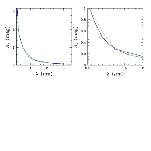
Figure 1: Comparison of the various extinction curves adopted; the right-hand panel is a zoomed-in version of the left-hand panel. Galactic extinction laws: solid lines – Savage & Mathis (1979); dotted lines – Rieke & Lebofsky (1985); short-dashed lines – Voshchinnikov & Il’in (1987); long-dashed lines – Fitzpatrick (1999). Starburst galaxy extinction law: dot/long-dashed lines – Calzetti et al. (1994).

In the left-hand panel of Fig. 1 we show these extinction laws in relation to each other over the wavelength range of interest for the present study, normalised at an extinction of 1 mag in the V band at 5500Å, $A_{V}=1$ mag. In the right-hand panel we zoom in to display the differences among the individual extinction laws from 0.5 to 2.0 $\mu$m. From a comparison of the individual extinction curves in the right-hand panel, it is clear that the differences are generally $\lesssim 0.05$ mag at wavelengths longward of $1\mu$m and shortward of $\sim 0.8\mu$m (with the exception of the Voshchinnikov & Il’in [1987] extinction law). In the intermediate wavelength range, the differences are mainly driven by the Rieke & Lebofsky (1985) Galactic extinction law on the one hand and the Voshchinnikov & Il’in (1987) curve on the other. Nevertheless, representative differences from the mean generally do not exceed 0.1 mag, even at these wavelengths, and are often significantly smaller.

If we place these differences among the extinction laws in their proper context, i.e., in comparison with the observational data presented in Section 2, we see that they are generally of the same order or smaller than the observational uncertainties. In addition, as we will see in Section 5, the vast majority of the sample clusters are characterised by $A_{V}\ll 1$ mag, so that the differences among the various extinction laws become negligible for our sample clusters, irrespective of the analysis approach adopted. This conclusion is further strengthened if we realise that the wavelengths crucial for a successful determination of, in particular, extinction values and metallicities are the bluest optical/UV and the redder NIR passbands (see, e.g., de Grijs et al. 2003c, Anders et al. 2004b), where the differences among the individual extinction curves are smallest.

3.2 Simple stellar population models

All of the methods used in this study rely on a comparison of the observational broad-band SEDs with a grid of model SEDs, in the sense that the star clusters are assumed to represent “simple” stellar populations, i.e., single-age, single-metallicity populations with a range of stellar masses determined by a given stellar IMF. The main differences among the various SSPs used for the comparison done in this paper are related to the use of different descriptions of the input physics, such as (i) a variety of stellar tracks or isochrones, which may or may not include critical phases in stellar evolution, such as the red supergiant (RSG) phase, Wolf-Rayet stars, and the thermally-pulsing AGB (TP-AGB) phase; (ii) slightly different IMF descriptions; and (iii) different (or no) treatment of nebular emission, particularly in the early phases of stellar evolution.

Each of the approaches used in this paper is based on a comparison with a specific set of stellar evolutionary synthesis models. We will use (i) the most commonly used set of models developed by Bruzual & Charlot (1993, 1996 [BC96], 2000 [BC00]; recently updated, 2003), (ii) the Starburst99 models of Leitherer & Heckman (1995) and Leitherer et al. (1999), which are specifically matched to analyse the young stellar populations in starburst and interacting galaxies, and (iii) the Göttingen SSP models galev (Kurth et al. 1999, Schulz et al. 2002, Anders & Fritze–v. Alvensleben 2003).

3.2.1 The Bruzual & Charlot SSP models

The basic assumptions of the modern sets of the Bruzual & Charlot SSP models (used in Sections 3.3, 3.5 and 3.6), were first developed in Charlot & Bruzual (1991). The versions of the code used in this paper, BC96 and BC00, include a description of SSP evolution for a range of metallicities from $Z=0.0004$ to $Z=0.10$. The BC96 models and more recent versions are (mostly) based on the evolutionary tracks of the Padova group (Bressan et al. 1993, Fagotto et al. 1994a,b,c; with additional empirical spectra for stellar masses between 0.1 and 0.7 M_⊙; Charlot & Bruzual 1991), and cover an age range from $1.25\times 10^{5}$ to $2\times 10^{10}$ yr, typically computed using 220 unequally spaced age intervals. The important TP-AGB phase (see Section 3.2.3) is treated semi-empirically. These models cover all of the important phases of stellar evolution from the zero-age main sequence to the post-AGB phase and beyond, for stars with effective temperatures of $2000\leq T_{\rm eff}({\rm K})\leq 50,000$. The stellar spectra are based on the theoretical spectral library compiled by Lejeune, Cuisinier & Buser (1997, 1998), which use the theoretical stellar atmosphere calculations of Kurucz (1979), Fluks et al. (1994), and Bessell et al. (1989, 1991). Lejeune et al. (1997, 1998) have corrected the stellar continuum shapes from the Kurucz (1979) models to agree with observed colours from the UV to the K band. SSPs, covering the wavelength range from the extreme UV (5Å) to the far-infrared (100$\mu$m) with a resolution depending on the spectral range, were calculated assuming a Salpeter (1955)-type IMF, $\xi(m)\propto m^{-\alpha}$ with $\alpha=2.35$ and masses ranging from $\sim 0.1{\rm M}_{\odot}$ up to 125 M_⊙.

3.2.2 The Starburst99 models

The Leitherer et al. (1999) Starburst99 models (used in Sections 3.4 and 3.6) constitute an improved and extended version of the suite of models initially published by Leitherer & Heckman (1995). These models were specifically developed for the evolutionary synthesis analysis of populations of massive stars, and are best suited to the conditions typically found in starburst environments. They are based on the Geneva stellar evolution models and the new model atmosphere grid compiled by Lejeune et al. (1997). The tracks of Meynet et al. (1994) were used for stars with masses in excess of 12–25 M_⊙ (depending on metallicity), with the enhanced mass loss prescription in order to better approximate most Wolf-Rayet properties (except the Wolf-Rayet mass-loss rate itself) compared to the standard mass loss scenario. For stars with masses in the range $0.8\leq m_{\ast}/{\rm M}_{\odot}\leq 12$, they used the standard mass-loss tracks of Schaller et al. (1992), Schaerer et al. (1993a,b) and Charbonnel et al. (1993). These tracks include the early AGB evolution until the first thermal pulse for stars with masses $m_{\ast}>1.7{\rm M}_{\odot}$. The Starburst99 models also include observational high-resolution UV spectra, to allow for the analysis of stellar and interstellar absorption lines and line profiles at various metallicities.

The SSP models cover an age range between $10^{6}$ and $10^{9}$ yr, with an age resolution of 0.1 Myr, for all five metallicities, $Z=0.001,0.004,0.008,0.02,$ and 0.04 over the entire spectral range from the extreme UV to the infrared. Nebular continuum emission is included in the models in a simplified fashion; its contribution becomes important when hot stars providing ionising photons (and thus line emission) are present (see Section 3.2.3).

The synthesised models that we use in Section 3.6 below were calculated using a standard Salpeter-type IMF, characterised by stellar masses in the range $1\leq m_{\ast}/{\rm M}_{\odot}\leq 100$.

3.2.3 The galev Göttingen SSP models

The galev SSPs (used in Sections 3.4, 3.6 and 3.7) are based on the set of stellar evolutionary tracks (Kurth et al. 1999), and in later versions the isochrones (Schulz et al. 2002, Anders & Fritze–v. Alvensleben 2003), of the Padova group (with the most recent versions using the updated Bertelli et al. [1994; and unpublished] isochrones; the latter also include the TP-AGB phase) for the metallicity range of $0.0001\leq Z\leq 0.05$, tabulated as five discrete metallicities ($Z=0.0004,0.004,0.008,0.02,$ and 0.05, corresponding to [M/H] $\approx$ [Fe/H] = $-1.7,-0.7,-0.4,0.0,$ and +0.4, respectively). For lower-mass stars ($0.08\leq m_{\ast}/{\rm M}_{\odot}\leq 0.5$), which contribute very little to the integrated light of young and intermediate-age SSPs governed by any standard, Salpeter-type IMF, the Padova models are supplemented with the Chabrier & Baraffe (1997) theoretical calculations that include a new description of stellar interiors of low-mass objects and use non-grey atmosphere models.

The galev models are furthermore once again based on the theoretical stellar libraries of Lejeune et al. (1997, 1998) for a broad range of metallicities. For stars hotter than $T_{\rm eff}=50,000$ K, pure black-body spectra are adopted, as for the Bruzual & Charlot models. The full set of models spans the wavelength range from 90Å to 160$\mu$m.

The Salpeter-type IMF assumed is characterised by a lower cut-off mass of $0.15{\rm M}_{\odot}$; the upper-mass cut-off ranges between 50 and 70 M_⊙, and is determined by the mass coverage of the Padova isochrones for a given metallicity.

Kurth et al. (1999) cover ages between $1\times 10^{7}$ to $1.6\times 10^{10}$ yr, with an age resolution of $10^{7},10^{8},$ and $10^{9}$ yr, for ages $\leq 10^{8}$, between $10^{8}$ and $10^{9}$ and $\geq 10^{9}$ yr, respectively. Schulz et al. (2002) and Anders & Fritze–v. Alvensleben (2003) extended the age range down to $4\times 10^{6}$ yr (and slightly reduced the upper age limit to 14 Gyr), while improving the age resolution to 4 Myr for ages up to 2.35 Gyr, and 20 Myr for greater ages.

The Schulz et al. (2002) version includes important improvements with respect to the older versions; they use the newer Padova isochrones which include the important stellar evolutionary TP-AGB phase. At ages ranging from $\sim 100$ Myr to $\sim 1$ Gyr, TP-AGB stars account for 25 to 40 per cent of the bolometric light, and for 50 to 60 per cent of the K-band emission of SSPs (see Charlot 1996, Schulz et al. 2002). Schulz et al. (2002) show that the effect of including the TP-AGB phase results in redder colours for SSPs with ages between $\sim 10^{8}$ and $10^{9}$ yr, with the strongest effect (up to $\gtrsim 1$ mag) being seen in $(V-K)$ for solar metallicity, and in $(V-I)$ for $Z\geq 0.5Z_{\odot}$. Shorter-wavelength colours and lower metallicity SSPs are less affected. Since most young to intermediate-age star cluster systems observed in HST passbands equivalent to the standard $V$ and $I$ filters, are in fact aged between about 100 Myr and 1 Gyr, and have often close-to solar metallicities, inclusion of the TP-AGB phase in the models is obviously important.

Finally, Anders & Fritze–v. Alvensleben (2003) included gaseous continuum emission and an exhaustive set of nebular emission lines to the galev suite, assuming comparable metallicities for the star cluster and the surrounding ionised gas. Nebular emission is shown to be an important contributor to broad-band fluxes during the first few $\times 10^{7}$ yr of SSP evolution, the exact details depending on the metallicity.

3.2.4 Model comparison

First, we present a basic comparison among the SSP models used in this paper. Kurth et al. (1999) and Schulz et al. (2002) concluded that, compared to the models of BC96 and Bruzual & Charlot (1993), respectively, their sets of galev models agree very well for solar metallicity and a Salpeter IMF, for $(B-V)$ colours, and from the UV up to $\sim 7000$Å, respectively. However, between 7000Å and 12,000Å, as well as in the NIR H and K band regime, the BC96 flux contribution is considerably lower than that of the Schulz et al. (2002) spectrum at those wavelengths, which they attribute to the different treatment of the TP-AGB evolutionary phase (with $T_{\rm eff}\sim 3000$ K).

Anders & Fritze–v. Alvensleben (2003) compare the most up-to-date galev models that include nebular line and continuum emission with the Starburst99 models. Despite the differences in the input physics and the different sets of stellar tracks and/or isochrones used by these teams, they conclude that the differences between both sets of models are minor at short optical wavelengths (e.g., $(B-V)$ colours) during the first Gyr of evolution, and are mainly due to the better time resolution of the Starburst99 models. Longer-wavelength comparisons show larger differences, due to the different input physics, and in particular a different treatment of RSGs and the TP-AGB phase.

In summary, it appears that over most of the optical wavelength range all of the commonly used SSP models are fairly similar, with minor differences depending on the detailed input physics and the treatment of the various evolutionary phases. At longer (NIR) and shorter (bluer) wavelengths, the differences become more significant, and will lead to systematic differences in the determination of the basic properties of SSPs, as we will see below.

Quantitatively, for a given set of input physics, varying parameters including the IMF slope, mass loss and convection prescriptions, one can justify differences of up to $\sim 0.05$ mag in $(B-V)$ (e.g., Yi 2003). However, the difference between – for instance – the Padova and Geneva stellar evolutionary tracks when used by an otherwise identical SSP code amounts to $\Delta(B-V)\sim 0.05$ mag, and even more in $\Delta(V-I)$ and $\Delta(V-K)$ (e.g., Leitherer et al. 1996, Schulz et al. 2002).

It is clear from the outset that the application of the various SSP models to our sets of sample clusters will result in significantly different masses and mass distributions, simply because of the different low and high-mass boundaries adopted for the Salpeter-type IMF. The mass ratios expected to result from the Starburst99 : the Bruzual & Charlot : the galev SSPs are 1 : 22.4 : 33.1, or in logarithmic mass units, mass estimates based on the Bruzual & Charlot SSPs will result in masses that are 1.35 dex higher than those from the Starburst99 models; the galev masses will be 1.52 dex more massive than the Starburst99 ones.

3.3 Method 1: Optical/NIR sequential analysis (“Sequential O/IR”)

The Sequential O/IR method is a two-step approach to derive the age, metallicity and extinction values associated with a given cluster. First, the extinction is estimated using the $BVI$ passband combination; subsequently, the extinction-corrected, intrinsic colours are compared, in a least-squares sense, to the BC96 SSP models in order to estimate the cluster age.

While the $(B-V)$ vs. $(V-I)$ colour-colour diagram is affected by the well-known age-metallicity degeneracy, the age and extinction trajectories are not entirely degenerate for this particular choice of optical colours. For SSPs older than $\sim 100$ Myr (i.e., $(B-V)_{0}\gtrsim 0.18$ mag), all age trajectories show the same, roughly linear growth of the $(V-I)_{0}$ vs $(B-V)_{0}$ colours, irrespective of their metallicity. As a consequence, for such ages, $(B-V)$ vs. $(V-I)$ SSP analysis enables us to derive the visual extinction (and therefore the intrinsic colours and magnitudes), prior to any age and metallicity estimates (cf. de Grijs et al. 2001).

Using the intrinsic colours we can now derive the most representative age (and metallicity), by minimising (in a least-squares sense),

$$\chi^{2}_{\rm min}(t,Z)={\rm min}\left\{\sum_{i=1}^{3}\left(\frac{{{\rm CI}_{i}}^{\rm intr}-{{\rm CI}_{i}}^{\rm SSP}(t,Z)}{\sigma_{{\rm CI}_{i}}}\right)^{2}\right\}\,,$$ (1)

where CI${}_{i}^{\rm intr}$ and CI${}_{i}^{\rm SSP}(t,Z)$ are the intrinsic and the model-predicted colour indices in a given colour denoted by $i$, respectively, for SSPs with age $t$ and metallicity $Z$; $\sigma_{{\rm CI}_{i}}$ are the 1$\sigma$ uncertainties.

If NIR photometry is available, the cluster age and metallicity can be derived simultaneously: for instance, the isochrones and iso-metallicity tracks define a grid in $(V-I)$ vs. $(V-J)$ space, thus allowing one to lift the age-metallicity degeneracy, as shown in Fig. 2. Finally, cluster masses are obtained from their luminosities via the age and metallicity dependent mass-to-light ratio.

Figure 2: $(V-I)_{0}$ vs. $(V-J)_{0}$ colour-colour diagram of the BC96 SSPs. The thin curves represent isometallicity tracks; the thick curves connecting filled symbols represent isochrones (from left to right, log $t/{\rm yr}$ = 8.5, 9.0, 9.5 and 10.0, respectively). As an example, the thin boxes represent the medians of typical 1$\sigma$ error distributions for SSPs of solar metallicity at ages of 600 Myr and 10 Gyr. The arrow indicates the effects of reddening on these models, for a visual extinction $A_{V}=1\,{\rm mag}$. For the sake of clarity, only SSPs older than 100 Myr are shown.

Our recent study of the intermediate-age star cluster population in M82’s region B provides a good example of what can be achieved if both optical and NIR data are available. In that case, both the age-extinction and the age-metallicity degeneracies can be lifted. Further details, and a discussion about how photometric errors propagate into extinction, age, metallicity and mass uncertainties are given in Parmentier, de Grijs & Gilmore (2003).

3.4 Method 2: Reddening-free Q parameter analysis (“Q-Q”)

The basic Q-parameter analysis is a powerful method to determine SSP ages and extinction values independently. The host galaxy’s internal extinction to a given cluster is derived from the $Q_{UBV}$ parameter (Johnson & Morgan 1953),

$$Q_{UBV} = (U-B)_{0}-[{\rm E}(U-B)/{\rm E}(B-V)]\times(B-V)_{0}$$ (2)

$$= (U-B)-0.72\times(B-V),$$

To estimate the internal reddening we assess the loci of the clusters in the $(B-V)$ vs $Q_{UBV}$ plane, compared to the intrinsic $(B-V)_{0}$ colours of the Starburst99 and galev SSPs.

Subsequently, age estimates are obtained by minimising the clusters’ loci in the plane of the reddening-free $Q_{UBV}$ and $Q_{UBVI}$ parameters, where the latter is defined as (Whitmore et al. 1999)

$$Q_{UBVI} = (U-B)_{0}-[{\rm E}(U-B)/{\rm E}(V-I)]\times(V-I)_{0}$$ (3)

$$= (U-B)-0.58\times(V-I),$$

with respect to the Starburst99 models. Unfortunately, due to a loop of the evolutionary tracks in Q–Q space, one cannot achieve accurate age estimates in the range of log(Age/yr) from $\sim 6.5$ to 7.2 (see Whitmore et al. 1999). The availability of H$\alpha$ observations will greatly facilitate our age estimates in this age range.

3.5 Method 3: H$\alpha$ luminosities in addition to broad-band fluxes (“BB+H$\alpha$”)

For those clusters for which we have H$\alpha$ flux or EW information available, we compared the five observed magnitudes ($UBVI\mbox{H}\alpha$) with the predicted SEDs from the BC00 SSPs at solar metallicity. For each available model age, we varied the reddening between E$(B-V)=0.0$ and 3.0 in steps of 0.02, and assume the Galactic extinction curve of Fitzpatrick (1999). Each model-age/reddening combination is scaled to match the cluster $V$-band magnitude, and then compared with the observations using a standard $\chi^{2}$ minimisation technique:

$$\chi^{2}_{\rm min}\bigl{(}t,{\rm E}(B-V)\bigr{)}={\rm min}\Bigl{\{}\sum_{\lambda}w_{\lambda}~{}(m_{\lambda}^{\rm model}-m_{\lambda}^{\rm obs})^{2}\Bigr{\}},$$ (4)

where $\lambda=U,B,V,I,\mbox{H}\alpha$ and $w_{\lambda}=[(0.05)^{2}+\sigma_{m_{\lambda}}^{2}]^{-1}$. Here, $\sigma_{m_{\lambda}}$ is the photometric uncertainty (in magnitudes) for a given bandpass; we have included an additional uncertainty of 0.05 mag, which represents the uncertainties in the models themselves (Section 3.2.4; see Fall, Chandar & Whitmore [2004] for validation of the method). Since bright objects can have very small photometric uncertainties, this keeps the weights from “blowing up” in the very bright object regime.

The predicted H$\alpha$ model flux is calculated from the total number of ionising photons under the assumption of photon-limited case B recombination. When converting to magnitudes, we determined the zero-point offset between the models and observations empirically, by comparing the observed difference in ($m_{{\rm H}\alpha}-m_{V}$) for the strongest H$\alpha$ emitters with model predictions. We then applied the empirically determined zero-point offset to the entire dataset, and found that for clusters younger than 10 Myr, with measurable H$\alpha$ emission, age estimates were in good agreement with those derived by Whitmore & Zhang (2002). (The measured H$\alpha$ fluxes for the clusters were converted to the vegamag system using the prescription given in the WFPC2 Data Handbook.)

We note that for those clusters without measurable H$\alpha$ EWs, we applied the simplified method based on the broad-band luminosities only, but using otherwise the same procedure.

3.6 Method 4: Three-dimensional SED analysis (“3DEF”)

The next step up in complexity of the fitting algorithms used involves the fitting of the observed cluster SEDs to the Starburst99 and BC00 models using a three-dimensional (3D) maximum likelihood method, 3DEF, with respect to a pre-computed grid of SSP models. This procedure was described in detail by Bik et al. (2003), based on their analysis of archival HST observations of the central star clusters in M51, and applied successfully to the intermediate-age star cluster system in M82 B by de Grijs et al. (2003b) and to the extended cluster sample in M51 by Bastian et al. (2004). The initial cluster mass $M_{i}$, age and extinction E$(B-V)$ were adopted as free parameters. For those clusters with upper limits in one or more filters, but still leaving us with a minimum of three reliable photometric measurements, we use a two-dimensional maximum likelihood fit (“2DEF”), using the extinction probability distribution for E$(B-V)$. This distribution was derived for the clusters with well-defined SEDs over the full wavelength range (see Bik et al. 2003 for a full overview of this procedure). The derivation of the most representative set of models for a given cluster is done via a least-squares ($\chi^{2}$) minimisation technique, in which the observed cluster SED is compared to the full grid of SSP models. In the application of the 3DEF-method Bik et al. (2003) and Bastian et al. (2004) assumed an uncertainty of 0.05 mag in the magnitudes of the cluster models (0.1 mag in the UV filters).

3.7 Method 5: Multidimensional SED analysis (“AnalySED”)

Finally, we have developed a sophisticated SED analysis tool that can be applied to photometric measurements in a given number $N(N\geq 4)$ of broad-band passbands (see de Grijs et al. 2003c, Anders et al. 2004b). We apply a 3D $\chi^{2}$ minimisation to the SEDs of our star clusters with respect to the galev SSP models, to obtain the most likely combination of age t, metallicity Z and internal extinction E$(B-V)$ for each object (see Anders et al. 2004b; Galactic foreground extinction is taken from Schlegel, Finkbeiner & Davis 1998).

In order to obtain useful results for all of our three free parameters, i.e., age, metallicity and extinction, we need a minimum SED coverage of four passbands.

Each of the models is assigned a probability, determined by a likelihood estimator of the form $p\sim\exp(-\chi^{2})$, where

$$\chi^{2}\bigl{(}t,Z,{\rm E}(B-V),m_{\rm cl}\bigr{)}=\sum_{\rm models}\frac{(m_{\rm obs}-m_{\rm model})^{2}}{\sigma^{2}_{\rm obs}}.$$ (5)

Clusters with unusually large “best” $\chi^{2}$ are rejected, since this is an indication of calibration errors, features not included in the models (such as Wolf-Rayet star dominated spectra, objects younger than 4 Myr, etc.) or problems due to the limited parameter resolutions. We include an additional 0.1 mag per passband for “model uncertainties” (0.2 mag for UV filters; see Section 3.2.4).

Subsequently, the model with the highest probability is chosen as the “best-fitting model”. Models with decreasing probabilities are summed up until reaching 68.26 per cent total probability (i.e., the 1 $\sigma$ confidence interval) to estimate the uncertainties on the best-fitting model parameters. For each of these best-fitting models the product of the relative uncertainties (${\rm\frac{age^{+}}{age^{-}}\times\frac{mass^{+}}{mass^{-}}\times\frac{Z^{+}}{Z^{-}}}$) was calculated (the superscripts indicate the upper (⁺) and the lower limits (^-), respectively). The relative uncertainty of the extinction was not taken into account, since the lower extinction limit is often zero. For each cluster, the data set with the lowest value of this product was adopted as the most representative set of parameters. In cases where the analysis converged to a single model, a generic uncertainty of 30 per cent was assumed for all parameters in linear space, corresponding to an uncertainty of ${}^{+0.1}_{-0.15}$ dex in logarithmic parameter space. See also de Grijs et al. (2003a,b,c) and Anders et al. (2004a) for applications of this algorithm to NGC 3310 and NGC 6745, and NGC 1569, respectively, and Anders et al. (2004b) for a theoretical analysis of its reliability.

We caution that the multi-passband combinations must not be biased to contain mainly short wavelength, nor mainly long-wavelength filters. Coverage of the entire optical wavelength range, if possible with the addition of UV and NIR data, is most preferable (de Grijs et al. 2003c, Anders et al. 2004b).

Finally, we emphasize once again that we will use this AnalySED method as the basis for our comparisons among the different approaches employed in this paper. This decision is based on the fact that the method was validated and tested extensively, both empirically (de Grijs et al. 2003a,c) and theoretically (Anders et al. 2004b), so that we understand the systematic uncertainties inherent to this approach in depth. In the following section, we will summarise the results from our extensive validation of the AnalySED method, in order to justify its use as our benchmark approach for comparison with the other methods descirbed in the previous sections in the remainder of this paper.

4 Establishing our benchmark approach with artificial data

Figure 3: Accuracy of the retrieval of the ages and masses of artificial star clusters based on a wavelength coverage as available for our NGC 3310 cluster sample. The artifical clusters are characterised by E$(B-V)=0.1$ mag, $Z=Z_{\odot}$, and ages of 8, 60, and 200 Myr, and 1 Gyr (objects 1–4). The different symbols represent the retrieved values based on a variety of a priori assumptions on the clusters’ metallicities.

Figure 4: Accuracy of the retrieval of the ages and masses of artifical star clusters based on a wavelength coverage as available for our Antennae cluster sample; technical details are as in Fig. 3.

In Anders et al. (2004b) we presented a detailed study of the reliability and limitations of our AnalySED approach. We computed a large grid of broad-band HST-based star cluster SEDs on the basis of our galev models for SSPs, including all relevant up-to-date input physics for stellar ages $\geq 4$ Myr. We constructed numerous artificial cluster SEDs, and varied each of the input parameters (specifically, age, metallicity, and internal extinction; see Section 3.7) in turn to assess their effects on the robustness of our parameter recovery. For each clean model artificial cluster SED we calculated 10,000 additional clusters, with errors distributed around the input magnitudes in a Gaussian fashion.

By analysing artificial clusters, using a variety of input parameters with our AnalySED approach, we found in general good agreement between the recovered and the input parameters for ages $\lesssim 10^{9}$ yr, i.e., exactly the age range of interest for the clusters in NGC 3310 and the Antennae galaxies analysed in this paper.

We considered several a priori restrictions of the full parameter space, both to the (correct) input values and to some commonly assumed values. We easily recover all remaining input values correctly if one of them is restricted a priori to its correct input value; this also provides a sanity check for the reliability of our code. We conclude that the age-metallicity degeneracy is responsible for some misinterpretations of clusters younger than $\sim 200$ Myr. If we restrict one or more of our input parameters a priori to incorrect values (such as by using, e.g., only solar metallicity, as often done in the literature), large uncertainties result in the remaining parameters.

In order to provide a robust theoretical benchmark for the observational study of systematic uncertainties presented in the remainder of this paper, here we re-validate our AnalySED approach using the exact filter combinations available for our NGC 3310 and Antennae cluster samples (Tables 1 and 2), i.e., by computing a large grid of broad-band star cluster SEDs in a similar fashion as done in Anders et al. (2004b) – although using only 1,000 additional artificial clusters to quantify our model uncertainties; the difference between this approach and the 10,000 additional artificial clusters used in Anders et al. (2004b) is negligible, however. Our artifical cluster SEDs were computed for ages of 8, 60, and 200 Myr and 1 Gyr (the age range covered by our sample clusters; see Sections 5.1 and 5.2), and for a fixed (internal) extinction of E$(B-V)=0.10$ mag and solar metallicity. The extinction value adopted roughly corresponds to the mean extinction derived for the individual clusters (Sections 5.1 and 5.2); extinction variations among the sample clusters are small, and their effects (for the derived range of extinction values) on the age and mass estimates are negligible (de Grijs et al. 2003a, Anders et al. 2004b). The adopted solar metallicity also corresponds roughly to the mean metallicity derived for the sample clusters, although it may not be correct in individual cases. In order to quantify the effects of metallicity variations, we attempted to retrieve the ages and masses of our artificial clusters by assuming both the correct (solar) and incorrect ($Z=0.008=0.4Z_{\odot}$) metallicities as a priori restrictions. In addition, we retrieved the ages and masses of the artificial clusters without any restriction to the resulting metallicity (“$Z$ free”). The latter provides a quantitative indication of the importance of the age-metallicity degeneracy.

The results of this re-validation are shown in Figs. 3 and 4 for filter coverage as for NGC 3310 and the Antennae galaxies, respectively. It is immediately clear that the accuracy of the parameter retrieval is significantly better for the NGC 3310 clusters than for those in the Antennae galaxies, which simply reflects the available filter sets (cf. de Grijs et al. 2003a,c, Anders et al. 2004b). Nevertheless, in all cases the ages are retrieved well within the modelling uncertainties, for any assumption on the clusters metallicity. For the coverage corresponding to the NGC 3310 clusters, the difference between input and retrieved ages is $\Delta\log({\rm Age/yr})\lesssim 0.3$, and in the majority of cases $\Delta\log({\rm Age/yr})\lesssim 0.15$. Except for the 60 Myr-old cluster, $\Delta\log({\rm Age/yr})\lesssim 0.3$ also for those clusters covered by the same passbands as the Antennae clusters (although the age-metallicity degeneracy is somewhat more important for the 1 Gyr-old cluster in this case). The corresponding uncertainty in the retrieved age of the 60 Myr-old artificial cluster is about twice as large as for the other clusters; its cause is unclear, since the retrieved extinction and metallicity values for this object are not significantly more uncertain than for the other objects.

A similar behaviour, i.e., with slightly larger uncertainties for the Antennae-equivalent wavelength coverage compared to the coverage of the NGC 3310 sample, is seen for the retrieved masses of the artificial clusters, although to a lesser extent. The mass uncertainties for all clusters older than 60 Myr are $\Delta\log(M_{\rm cl}/M_{\odot})\lesssim 0.10-0.15$. For the youngest, 8 Myr-old object, we are only able to retrieve the masses to within several 0.1 dex in mass (somewhat more accurately for the NGC 3310-equivalent wavelength coverage, particularly if the adopted metallicity is close to the actual value); this is most likely caused by the uncertainties inherent to our present knowledge of stellar evolution in this age range (such as, e.g., the importance of the RSG phase), and the relatively coarse age resolution compared to the rapidity of changes in stellar evolution around 6–12 Myr.

Thus we have shown, based on well-understood artificial data, that we understand quantitatively the uncertainties inherent to using our AnalySED approach for age and mass determinations of star clusters based on broad-band imaging. We will be using this approach as our benchmark for comparing our results to those obtained using alternative methods commonly in use in the community.

In Section 3.2.4 we concluded that the differences among the various prescriptions used for the input physics in modern sets of SSP models are very small indeed and apparently not biased systematically. As a consequence of the analysis performed in this section, we conclude then that any differences in the individual (as well as in the mean) cluster ages and masses that we will find in subsequent sections (over and above the modelling uncertainties quantified here) are most likely caused by intrinsic differences among the various methods.

5 Comparison of the relative age and mass distributions

5.1 Extensive wavelength coverage: NGC 3310

To start our comparison of methods, we will focus on the extensive wavelength coverage of the NGC 3310 star cluster system. With coverage from the F300W HST mid-UV passband to the NIR F205W passband, the resulting broad-band SEDs were shown to have sufficient leverage to distinguish metallicity, extinction, and stellar population (age) effects (de Grijs et al. 2003c).

While a wavelength coverage as extensive as possible is preferred, the use of HST-flight system magnitudes (cf. Section 2) limits the application of the NGC 3310 comparison to the use of the galev SSP models (see Section 3.2.3), which we folded through the HST/WFPC2 filter curves ourselves (e.g., de Grijs et al. 2003c, Bastian et al. 2004).

We emphasize, however, that we prefer to use the original HST-flight filter system, rather than conversions to “standard” systems; in Section 7 we will discuss the systematic effects unavoidably introduced when converting HST-flight system magnitudes to the “standard” Johnson-Cousins system.

Figure 6 shows the resulting age distributions for the 17 NGC 3310 star clusters used for this exercise, obtained using a variety of approaches. In Fig. 6a, we display the relative age distribution of the NGC 3310 clusters based on the full multi-dimensional SED analysis (Section 3.7), in which we left all of the cluster ages, masses, metallicities and extinction values as free parameters. The vertical dotted line at log(Age/yr) = 6.6 denotes the lower age limit of the galev SSP models; the vertical error bars indicate the Poissonian uncertainties.

Panel (b) provides a direct comparison of the effects of metallicity variations. Here, as well as in the other panels in this figure, we have adopted solar metallicity for the individual star clusters. While this is not necessarily correct in general, restricting the metallicity to the solar value allows a more robust comparison among the various models and methods. The differences in the relative age distributions between Figs. 6a and b are therefore entirely and exclusively due to the different assumptions on the clusters’ metallicities. They reflect the well-known effects of the age-metallicity degeneracy (e.g., Ferreras & Yi 2004; see de Grijs et al. [2003a,c] for detailed studies of this effect in NGC 3310 and NGC 6745). Based on the multi-dimensional analysis presented in Fig. 6a, most (70 per cent) of the NGC 3310 clusters in our current sample are characterised by metallicities $Z\lesssim 0.01$, with the remainder split evenly between solar metallicity ($Z=0.02$) and $Z\sim 0.05$, see Fig. 5. Support for these metallicity estimates is provided by the unusually low (subsolar) metallicity found independently in star-forming regions surrounding the nucleus of NGC 3310, while the nucleus itself appears to have solar metallicity (e.g., Heckman & Balick 1980, Puxley, Hawarden & Mountain 1990, Pastoriza et al. 1993). Similarly, the age-extinction degeneracy may contribute to some extent, although its effect is likely less than that of the age-metallicity degeneracy (cf. de Grijs et al. 2003c). The extinction in this sample of NGC 3310 clusters, E$(B-V)$, decreases with age – although with a large scatter – from E$(B-V)\sim 0.35$–0.40 mag at $\sim 10^{6.5}$ yr, to E$(B-V)<0.1$ mag at $\sim 10^{8}$ yr.

Figure 5: Metallicity estimates of the NGC 3310 and Antennae sample clusters, based on the results obtained from the AnalySED multi-dimensional approach. Note that these are first-order estimates (yielding an internally consistent overall metallicity distribution; see Anders et al. 2004b), and that the uncertainties in the individual cluster metallicities are on the order of one step in our metallicity grid, covering metallicities of $0.004Z_{\odot},0.2Z_{\odot},0.4Z_{\odot},Z_{\odot}(Z=0.02)$, and $2.5Z_{\odot}$.

Figure 6c can be compared directly with Fig. 6b; the only difference between these two panels is that we used the “3DEF” method (Section 3.6) instead of the AnalySED multi-dimensional approach. We used the galev SSP models in both cases. It is encouraging to see that the use of either method results in very similar relative age distributions. More quantitatively, the two peaks in the age distribution are reproduced to a very high degree of confidence ($>99$ per cent), although their relative amplitudes are subject to small-number statistics; as a result, the straightforward application of a Kolmogorov-Smirnov (KS) test yields a probability that these data points were drawn from statistically different distributions of $\sim 80$ per cent, but with a very large uncertainty because of the small number of data points used.

Table 3: Characteristics of the overall relative mass distributions of our NGC 3310 cluster sample

Method	SSPs	$Z$	log(Mass/M⊙)
			Mean	$\sigma$
AnalySED	galev	free	5.13	0.28
AnalySED	galev	$Z_{\odot}$	4.92	0.29
3DEF	galev	$Z_{\odot}$	4.89	0.23
3DEF	Starburst99	$Z_{\odot}$	5.04	0.24

Finally, in panel (d) we have replaced the galev SSP models by the Starburst99 models (Section 3.2.2), which results in a markedly different age distribution. This is most likely caused by two effects, which are in essence the most significant differences between these two sets of SSP models. The galev SSP models include the contributions of an extensive set of nebular emission lines and gaseous continuum emission, which have been shown to be important in the first few $\times 10^{7}$ yr of an SSP’s evolution (Anders & Fritze-v. Alvensleben 2003); the Starburst99 set of SSP models does include nebular continuum emission, but only in a simplified fashion. The other main difference between both sets of SSP models is related to their treatment of the RSG phase, which is of significant importance around $10^{7}$ yr: it is clear from panels (b) and (c) that using the galev models leaves a gap in the clusters’ age distribution around the time that the RSG phase is expected to be important. This is caused by a combination of both the age-metallicity degeneracy and the sparser age resolution of the galev models compared to that of the Starburst99 SSPs. Lamers et al. (2001) have shown that the Geneva models of fully convective stars are not cool or red enough compared to the observations, particularly at lower metallicities (see also Massey & Olsen 2003). This may have significant consequences for techniques which allow the metallicity to be a free parameter, obviously depending on the age range of the respective clusters. Whitmore & Zhang (2002) have shown that cluster models calculated with the Padova tracks fit the observations better than those calculated with the Geneva tracks.

The relative mass distributions, shown in Fig. 7, are much more similar to each other than the corresponding age distributions when we compare the various methods and SSP models used. The cluster masses have all been corrected to the stellar IMF used by the galev SSPs (see Section 3.2.4). The effect of the age-metallicity degeneracy is seen to some extent between panels (a) and (b,c,d): as we established above, this degeneracy causes the cluster ages to be underestimated if the metallicity is overestimated (as is likely the case if we assume solar metallicity for the NGC 3310 clusters), which in turn causes the cluster masses to be underestimated. However, this effect is minor in our NGC 3310 cluster sample. In spite of the inherent problems of applying KS tests to astrophysical data such as presented here, the results of such tests are illustrative in a comparative fashion: the difference in the adopted metallicity reduces the probability of distributions (a) and (b) to have been drawn from the same population to only 19.0 per cent. The agreement between distributions (b), and (c) and (d), are more satisfactory, with probabilities of these having been drawn from the same population of 93.0 and 67.3 per cent, respectively. In addition to the KS statistics, we can also compare the overall statistics of the distributions in Fig. 7, as shown in Table 3, which shows that we can reproduce the mean (“peak”) and spread of the distributions consistently and well within the uncertainties (represented by the $\sigma$ values), even where we adopted different metallicity distributions; if we simply compare the peak values of the mass distributions obtained from the various methods, we find a spread among these values of $\sigma_{M}\equiv\Delta\langle\log(M_{\rm cl}/{\rm M}_{\odot})\rangle\leq 0.06$ (where we have only used the peak values obtained assuming similar boundary conditions, i.e., for $Z_{\odot}$; the peak values were obtained from Gaussian fits to the distributions of the individual cluster masses). If we had simply taken the mean of the age distributions and done the same comparison, the resulting spread would have been $\sigma_{t}\equiv\Delta\langle\log({\rm Age/yr})\rangle\leq 0.15$ (although we note that this result is unphysical, in view of the significantly non-Gaussian distributions, so that a single “mean” value does not convey much useful information). Thus, we conclude that the peaks in the relative mass distributions can be derived much more consistently than those in the relative age distributions. This is caused by the way in which the masses are determined (by scaling up either the entire observed SED or the $V$-band flux to the models), and the fairly narrow age range covered by the NGC 3310 clusters (ensuring a relatively small range of cluster mass-to-light ratios).

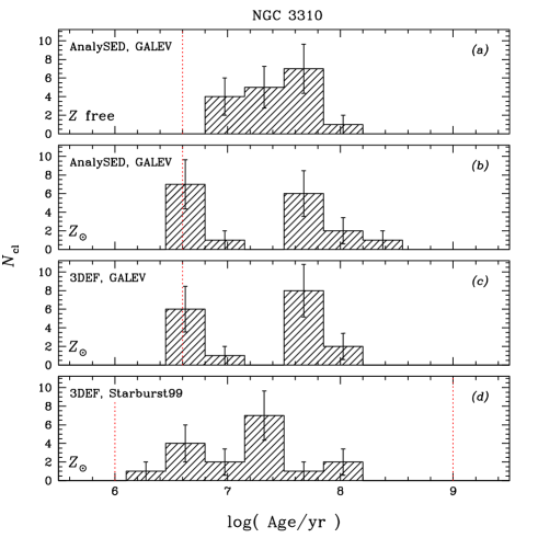
Figure 6: Resulting age distributions of the NGC 3310 star clusters, using a variety of methods and SSP models, as indicated in the individual panels. The vertical dotted lines correspond to the fitting boundaries of the models. Metallicities are indicated in the panels.

Figure 7: Resulting mass distributions of the NGC 3310 star clusters, using a variety of methods and SSP models, as indicated in the individual panels. Metallicities are also indicated in the panels.

5.2 Restricted wavelength coverage, including H$\alpha$ observations: NGC 4038/9

While ideally one would like to have the most extensive wavelength coverage possible, realistically one cannot expect to obtain more HST coverage than by, say, four passbands for any given cluster system. Under this assumption, we have shown – both empirically (de Grijs et al. 2003a,c) and theoretically (Anders et al. 2004b) – that the optical $UBVI$ passbands (or their equivalents in the HST flight system) provide the most suitable passband combination to use as the basis for our broad-band SED analysis. Additional NIR observations would add significantly more leverage, but in practice such observations need to be obtained using different detectors, and are thus more difficult to obtain. We focus therefore on data sets that can be obtained with minimal observing time, while maximising the scientific output.

In this section, we will explore the differences between the various methods, using $UBVI$ coverage of 20 star clusters in the Antennae interacting galaxies (NGC 4038/9), selected to span a large age range in the original analysis where their properties were first published (see Whitmore et al. 1999, and references therein). The “standard” $UBVI$ cluster magnitudes were obtained by converting the HST-flight system magnitudes using the Holtzman et al. (1995) conversion equations. For a subset of these clusters we have also obtained H$\alpha$ EWs, which can – in principle – be used to constrain their ages more accurately and robustly, although strong and patchy background H$\alpha$ fluxes (as observed in the Antennae galaxies) can render the actual contributions to the H$\alpha$ fluxes by the clusters themselves very uncertain.

Figure 8 shows the relative age distributions resulting from the application of the various methods described in Section 3. The top three panels of Fig. 8, (a), (b), and (c), show similar trends as pointed out for the same method+models combinations used for the NGC 3310 clusters in the previous section. The effects of the age-metallicity degeneracy are somewhat less pronounced in this case, since our multi-dimensional AnalySED analysis (Section 3.2.3) indicates that the cluster metallicities in the Antennae galaxies are roughly equally split between solar metallicity and $Z\sim 2.5Z_{\odot}$ (with only a few clusters characterised by subsolar metallicities, $Z\lesssim 0.01$). These metallicity estimates are supported by high-resolution spectroscopy obtained by Mengel et al. (2002). Thus, by assuming solar metallicity for all Antennae clusters, we will have overestimated the ages for those clusters with supersolar metallicity, and underestimated the ages of the few subsolar metallicity clusters. This is reflected by the different age distributions between panels (a) vs. (b) and (c). Again, application of these methods leaves a clear gap in the age distributions around the age where the RSGs become apparent.

The multi-dimensional SED analysis further shows a weak correlation between E$(B-V)$ and cluster age (although with a large scatter), from E$(B-V)\lesssim 1$ mag at $\sim 10^{6.5}$ yr to E$(B-V)\lesssim 0.4$ mag at $\sim 10^{9.5}$ yr.

In Fig. 8d, we display the results from the “Sequential O/IR” method (Section 3.3). Based on the availability of $BVI$ photometry, this method also allows us to determine the extinction toward the sample clusters independently. The weak trend found by our multi-dimensional SED approach is also found using this method, although the individual extinction values are generally slightly smaller, E$(B-V)\lesssim 0.2$ mag.

Yi et al. (2004) have shown that the $(U-B)$ versus $(B-V)$ two-colour diagram can be used to break the age-metallicity degeneracy for metal-poor populations. However, since our sample clusters are metal rich, we cannot apply this technique here. All of their ageing trajectories (based on the BC00 SSP models), whatever their metallicity, are at the same locus of the diagram, at least for stellar populations older than 100 Myr.

While the double-peaked age distribution obtained in panels (a)–(c) is to some extent reproduced, the two-step process of the Sequential O/IR method results in a more evenly spread age distribution. This is partially due to the fact that some of the sample clusters are apparent outliers in the diagnostic diagrams, and as a consequence their ages are not well constrained.

Finally, Figs. 8e and f show the age distributions resulting from using the reddening-free $Q$-parameter analysis and the broad-band+H$\alpha$ method (Sections 3.4 and 3.5), respectively. These distributions are, in very broad terms, consistent with those obtained using the other methods discussed before, in the sense that they show multiple peaks at roughly similar ages (although they do not match in detail). The most deviant distribution is in fact that resulting from the “Sequential O/IR” method, which is based on a smaller number of photometric data points per cluster than the other methods.

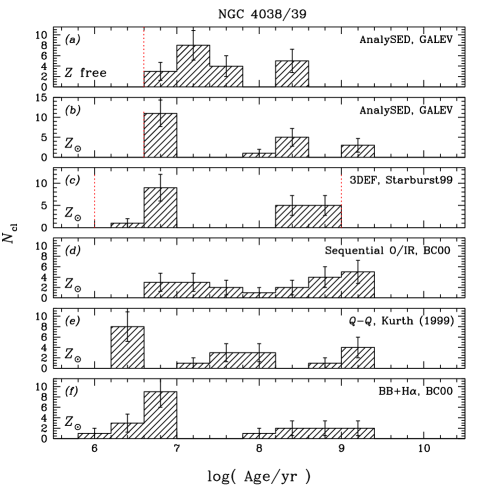
Figure 8: Resulting age distributions of the Antennae star clusters, using a variety of methods and SSP models, as indicated in the individual panels. The vertical dotted lines correspond to the boundaries of the models. Metallicities are indicated in the panels.

Figure 9 shows the corresponding mass distribution for our sample of Antennae clusters, based on a variety of methods. Because of the small-number statistics and, in particular, the different mass range covered by all of the mass distributions in Fig. 9 the simple KS statistic indicates that all distributions are different from our base line distributions, Figs. 9a and b, at the $>98$ per cent level (even if we restrict ourselves to the largest possible mass range in common between any two sets of mass determinations, and common metallicity assumptions). However, as for NGC 3310, the overall characteristics of the mass distributions are fairly consistently reproduced, in particular the mean mass (see also Table 4); similarly as for NGC 3310, we find a spread in the mean mass among the various approaches of $\sigma_{M}\equiv\Delta\langle\log(M_{\rm cl}/{\rm M}_{\odot})\rangle\leq 0.14$ (once again, for the fits done assuming $Z_{\odot}$ only). The equivalent spread for the (unphysical) mean in the age distributions would be $\sigma_{t}\equiv\Delta\langle\log({\rm Age/yr})\rangle\leq 0.35$. It appears, therefore, that – once more – the peaks in the relative mass distributions (as opposed to the detailed shapes of the distributions) can be obtained with a much higher degree of confidence than those of the relative age distributions.

The overall characteristics of the mass distributions for the current sample of Antennae clusters are summarised in Table 4, which were obtained using the same fitting algorithms as for the fits to the NGC 3310 mass distributions. We note that, due to insufficient information in the Kurth et al. (1999) SSP models at the highest time resolution (used in this paper), we were unable to determine the cluster masses for the $Q-Q$ method.

Figure 9: Resulting mass distributions of the Antennae star clusters, using a variety of methods and SSP models, as indicated in the individual panels. Metallicities are also indicated in the panels.

Table 4: Characteristics of the overall relative mass distributions of our Antennae cluster sample

Method	SSPs	$Z$	log(Mass/M⊙)
			Mean	$\sigma$
AnalySED	galev	free	5.20	0.26
AnalySED	galev	$Z_{\odot}$	4.72	0.31
3DEF	Starburst99	$Z_{\odot}$	4.97	0.47
Seq. O/IR	BC00	$Z_{\odot}$	5.12	0.32
Q–Q	Kurth (1999)	$Z_{\odot}$
BB+H$\alpha$	BC00	$Z_{\odot}$	4.91	0.32

6 One-to-one comparisons of mass and age estimates

Having established that the peak (or most frequent value) of the relative age and, in particular, mass distributions of a given star cluster system can be retrieved relatively robustly using broad-band SEDs, we will now explore to what extent this applies to the individual cluster properties themselves. It is clear from the outset that where multiple estimates for the cluster extinction values, and to a lesser extent also for their metallicities, exist, these estimates vary significantly. However, despite this being the case from an observational point of view, the effects on the SED of varying the extinction and metallicity, if their uncertainties are not more than a few tenths in magnitude or one step in metallicity, respectively, are small, and can thus still result in reasonably secure age and mass estimates for all but the youngest clusters (cf. Anders et al. 2004b). In other words, the age and mass estimates are relatively robust to variations in the extinction and metallicity estimates. Therefore, we will only discuss the one-to-one comparisons of the ages and masses of the individual clusters in either of our samples. We also note that the youngest SEDs ($\lesssim 10^{7}$ yr) can be affected quite significantly (and not in any systematic fashion) by even small changes in extinction and/or metallicity, however (see Anders et al. 2004b).

Figure 10 shows the one-to-one comparisons of the NGC 3310 cluster ages and masses, adopting solar metallicity, and using the AnalySED approach as our basis for the comparison. It is immediately clear that the methods using the same set of SSPs, Figs. 10a and c for the ages and masses, respectively, result in highly reproducible age and mass estimates (well within the 1-$\sigma$ error bars). With few exceptions, the individual ages and masses match very well within the model uncertainties.

In the most extreme case considered for the NGC 3310 star cluster system, namely by using a different method (AnalySED vs. 3DEF) and a different set of SSP models (galev vs. Starburst99; shown in Figs. 10b and d), the individual age and mass estimates still match up well within the model uncertainties, although with a slightly larger scatter. The “3DEF,Starburst99” approach results in slightly higher masses than the AnalySED approach, although this is only a $\sim 1\sigma$ deviation.

Figure 11 shows a similar set of comparisons for the Antennae clusters, now using the entire range of methods and models at our disposal. At first sight, we notice three characteristics when comparing these panels to the panels of Fig. 10. First, the uncertainties in the ages and masses estimated by the AnalySED approach (see Anders et al. 2004b for a full description and justification) are significantly larger than those resulting from most other methods used, except for the 3DEF approach. Secondly, the uncertainties are much greater than those for the individual age and mass estimates obtained for the NGC 3310 clusters. This reflects the difference in wavelength coverage of the broad-band SEDs for both sets of clusters: with the smaller wavelength coverage of the Antennae clusters, their best-fitting ages and masses are not as well constrained as for the more extensively covered NGC 3310 clusters. It therefore appears that the uncertainties estimated using the Sequential O/IR, the Q–Q and the BB+H$\alpha$ methods are too small in view of the ill-defined broad-band SEDs over the fairly small wavelength range covered. We should point out, however, that the uncertainties resulting from the BB+H$\alpha$ method (i.e., for clusters with measured H$\alpha$ EWs) are likely to be smaller than those from the broad-band-only methods, since this method uses H$\alpha$ EWs to further constrain the cluster ages. This method is therefore most accurate in a very narrow age range (i.e., more accurate than methods based on broad-band photometry alone), around $\sim 10$ Myr. Finally, it appears that the mass estimates of the individual clusters are better matched than their age estimates. This, in turn, provides the more robust relative mass distributions discussed in the previous Sections.

Thus, we believe that the main differences among the resulting age and mass estimates for individual clusters are caused by the difference in the wavelength range covered, but – as we will show in Section 7 – the uncertainties introduced by transforming the HST-flight system magnitudes to “standard” ground-based UBVI photometry may affect the robustness of the results to a similar, if not greater, degree. While the individual cluster ages and masses based on the “ideal” $UBVI$ (or equivalent) coverage advocated in de Grijs et al. (2003c), and Anders et al. (2004b) may be subject to significant uncertainties, the relative age and mass distributions are much more consistently established, so that statistical analyses of large-scale cluster systems based on multi-passband broad-band imaging do have the potential to provide robust scientific insights in their host galaxies’ formation, evolution, and star-formation histories.

Figure 10: One-to-one comparisons between the age (left) and mass (right) estimates of the NGC 3310 clusters, for solar metallicity, obtained from the various methods and SSP models, using our AnalySED approach as the basis for comparison. The dotted lines are the loci of equality.

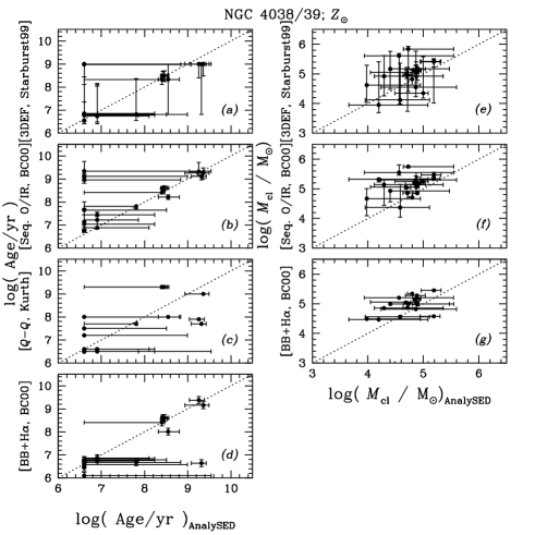
Figure 11: One-to-one comparisons between the age (left) and mass (right) estimates of the Antennae clusters, for solar metallicity, obtained from the various methods and SSP models, using our AnalySED approach as the basis for comparison. The dotted lines are the loci of equality.

Finally, in Table 5 we compare the age estimates for the individual clusters in our Antennae cluster sample with H$\alpha$ EW $>1.0$Å, for the full set of SSP analysis methods used. We have indicated the clearly discrepant age estimates in italic font. The final two columns of this table include the mean age and its standard deviation based on the individual age determinations; for those clusters with clearly discrepant values, we also give these numbers excluding these discrepant determinations. In addition, we have also included those cluster for which we determined ages of log( Age/yr ) $\leq 6.6$ but for which no strong H$\alpha$ EW measurements were provided.

Table 5: Age comparison for the individual clusters in our Antennae cluster sample with EW${}_{{\rm H}\alpha}>1.0$Å.
Values in italics are clearly discrepant values.

ID	EWHα	Q-Q	BB+H$\alpha$	AnalySED; Z free	AnalySED; $Z_{\odot}$	3DEF	O/IR		log( Age/yr )
	(Å)	log( Age/yr )							Mean	$\sigma$
G2-04	2.9	6.5	6.7	7.1	6.9	6.8	7.2		6.87	0.24
G2-05	2.5	7.5	6.8	7.1	6.6	6.8	7.6		6.98	0.29
									(6.83	0.18)b
G2-07	1.3	6.5	6.5	7.1	6.6	6.8	7.1		6.77	0.26
G2-08	2.9	6.5	6.8	7.2	6.6	6.8	7.0		6.82	0.23
G2-10	1.4	6.6	6.8	6.9	6.9	6.8	7.4		6.90	0.24
G2-12	2.5	6.6	6.8	7.3	6.6	6.8	6.8		6.82	0.23
G2-14	3.7	6.5	6.1	6.9	6.6	9.0	9.3		7.40	1.26
									(6.53	0.29)b
G2-15	3.5	6.5	6.5	7.1	6.6	6.6	6.8		6.68	0.21
Others with
log( Age/yr ) $\leq 6.6$,		G2-17	G2-19	G2-17a	G2-09,	–	G2-17a
but no H$\alpha$					G2-19

Notes: ^a Here, we used a limit of log( Age/yr ) $\leq 6.9$ because of the offset introduced by the age-metallicity degeneracy; ^b After exclusion of the values in italic font.

One can see immediately that the correspondence between the age estimates for a given cluster among the different analysis approaches is close. We note that the age estimates obtained using the sequential O/IR and AnalySED approaches, with metallicity as a free parameter are offset with respect to most of the other methods. This simply reflects the age-metallicity degeneracy for these young ages. Nevertheless, the fact that we obtain very similar age estimates using a variety of independent approaches that may or may not include H$\alpha$ luminosities as an additional contraint is reassuring. In principle, this validates the different approaches used here: nearly all clusters that should be young based on the presence of strong H$\alpha$ emission are indeed young (with between 0 and 2 outliers for all methods), and the ones predicted to be young based on these methods all have H$\alpha$ (except for, again, between 0 and 2 outliers). The outliers are characterised by the largest error bars, which is an additional argument in support of the robustness of the variety of models employed here. Unfortunately, there are no young extragalactic star clusters available in the current literature for which independent age estimates have been obtained via either spectroscopy or detailed analysis of their resolved colour-magnitude diagrams; the use of H$\alpha$ EWs, as done here, is therefore the closest we can get to an independent validation of our approach.

As an example of the uncertainties inherent to the use of broad-band (and H$\alpha$) fluxes to obtain the individual cluster ages, we direct the reader’s attention to cluster G2-14, for which we found the most discrepant age estimates among the variety of approaches used. This cluster shows strong H$\alpha$ emission, and must therefore be young. Nevertheless, two of the approaches employed assigned this cluster an age of greater than 1 Gyr. Upon close inspection, those discrepant estimates originated from the two approaches that essentially leave the metallicity as a free parameter. This hints at an origin related to the age-metallicity degeneracy. However, we also point out that the error bars assigned by the AnalySED approach are among the largest in our cluster sample. Statistically, the AnalySED age estimate (with metallicity as a free parameter) is therefore also consistent with a young age.

On the other hand, all of the different approaches employed here, for instance, estimate the age of cluster G2-17 to be in the range $6.6\lesssim\log({\rm Age/yr})\lesssim 6.9$ (see the Appendix for details), despite not having strong H$\alpha$ emission. In spite of this, the uniformity of this result among the different methods is encouraging; it implies a high degree of reproducibility.

7 Filter system conversions

Largely owing to the unavailability of SSP models computed for the HST-flight system magnitudes, many of the early studies based on HST imaging observations of extragalactic star cluster systems used the equations given by Holtzman et al. (1995) to convert HST stmag magnitudes to the “standard” Johnson-Cousins system. Despite recent updates of many of the leading SSP models, which now include theoretical magnitudes in the stmag system, many workers in the field, including ourselves in this paper (see our photometry of the Antennae clusters), continue to use the Holtzman et al. (1995) conversions.

It is clear, however, that any conversion based on generic spectral properties of a given stellar population will introduce biases and additional uncertainties that could, in principle, be avoided by retaining one’s photometry in the filter system used for the observations. In this section, we explore the extent of these additional uncertainties by comparing our model fitting results for the full NGC 3310 cluster sample, presented in de Grijs et al. (2003c), based on both the original HST/WFPC2 photometry and on the transformed magnitudes in the Landolt (KPNO) $UBVRI$ system used by Holtzman et al. (1995).

In order to do so, we folded the galev SSP models through these filter transmission curves, which were kindly made available by Jon Holtzman (priv. comm.). Despite being a standard system, the appropriate filter transmission curves have not been published in their entirety. We transformed our F336W, F439W, F606W and F814W magnitudes using Eqs. (6)–(9) below (for the WF3 chip of the WFPC2 camera), using an iterative approach; following Holtzman et al.’s (1995) recommendations, we did not transform the F300W magnitudes, but used the HST flight system magnitude for this part of the broad-band cluster SEDs. The conversions from the F336W, F439W, and F814W filters to their $UBI$ counterparts are based on the observational transformations from the WFPC2 flight system (Holtzman et al.’s Table 7), while the transformation of the F606W magnitudes to the $V$ filter relies on the conversion of the synthetic WFPC2 system to the standard $V$ band (their Table 10).

$$U= -2.5\times\log(\mbox{counts s}^{-1})-0.240\times(U-V)+\hfill$$ (6)

$$0.048\times(U-V)^{2}+18.764+2.5\times\log(2.003)$$

$$B= -2.5\times\log(\mbox{counts s}^{-1})+0.003\times(B-V)+\hfill$$ (7)

$$-0.088\times(B-V)^{2}+20.070+2.5\times\log(2.003)$$

$$V= -2.5\times\log(\mbox{counts s}^{-1})+0.254\times(V-I)+\hfill$$

$$+0.012\times(V-I)^{2}+22.093+2.5\times\log(2.003)$$

$$(\mbox{for }(V-I)\leq 2.0)$$

$$I= -2.5\times\log(\mbox{counts s}^{-1})-0.062\times(V-I)+\hfill$$ (9)

$$0.025\times(V-I)^{2}+20.839+2.5\times\log(2.003)$$

As before, we will first discuss the characteristics (i.e., predominantly the mean and spread) of the age and mass distributions of the entire cluster population, and conclude with a one-to-one comparison of the results obtained for the individual clusters. For the analysis presented in this section, we have adopted the AnalySED multi-dimensional modelling approach, using the galev SSP models. We attempted to obtain the cluster ages and masses under three sets of assumptions: (i) unrestricted fits, i.e., we left all of the cluster ages, masses, metallicities and extinction values as free parameters; (ii) as for (i), but assuming solar metallicity for all clusters; (iii) as for (ii), but now also assuming a generic (arbitrarily low) extinction value for each cluster of E$(B-V)=0.1$ mag.

In Fig. 12 we present the results for the relative age distributions, in the left-hand column using the HST-flight system magnitudes as our basis, and in the right-hand column using the transformed F300W-UBVI photometry. From top to bottom, the fits become more and more restricted, following the assumptions laid out above. Despite this being the same sample as analysed in de Grijs et al. (2003a,c), the resulting age distribution in panel (a) is different from that published previously. The main reason for this difference is that the fits discussed in this section do not include the NIR passbands, so that we are less sensitive to metallicity variations (Anders et al. 2004b). In other words, the strong peak seen at log(Age/yr) $\sim 6.6$ is caused by the age-metallicity effect, and also by the fact that the youngest age in our models corresponds to log(Age/yr) = 6.6 (so that younger clusters will automatically be assigned the minimum age in the models). This applies to the strong peaks seen at this age in all of the panels of Fig. 12. We note that the overall metallicity of NGC 3310 is known to be significantly subsolar (see Section 5.1), but we will use the assumption of solar metallicity in this section to emphasize a number of technical concerns relevant for similar studies in this field.

Apart from this obvious signature of the age-metallicity degeneracy, the overall relative age distribution, i.e., the mean value and its spread, based on the HST flight system photometry is retrieved relatively robustly under the various assumptions employed (see Fig. 12, left-hand panels); the range of ages found for the NGC 3310 clusters is consistent with independently determined age estimates for the star-forming regions in this galaxy (see de Grijs et al. 2003a,c for a detailed discussion). However, if we now examine the age distributions based on the transformed F300W-UBVI magnitudes, we see that (i) our results are severely affected by the age-metallicity degeneracy, and (ii) that the “transformed ages” do not correspond to even remotely similar ages as obtained from the HST-flight magnitudes. Only by severely restricting our model fits (Fig. 12c2) are we able to retrieve a similar age distribution as we obtained from the direct match of our SSP model grid to the HST-flight system magnitudes. This provides, therefore, a very strong argument against using photometry based on even robust filter conversions; the effect of such transformations is the unavoidable introduction of biases and additional uncertainties, which thus makes the various fitting routines less reliable and robust.

Figure 12: Comparison of the relative age distribution of the NGC 3310 clusters, based on the HST flight system photometry (left-hand column, panels a1, b1, and c1) and on the converted $UBVI$ magnitudes (right-hand column, panels a2, b2, and c2). Panels a1 and a2 are based on model fits in which all of the cluster ages, masses, metallicities and extinction values were left as free parameters; in panels b1 and b2 we restricted the fits to solar metallicity, and in panels c1 and c2 we also adopted a generic extinction of E$(B-V)=0.1$ mag.

If we now consider the resulting mass distributions, shown in Fig. 13, we see – somewhat to our surprise – that to first order these can be reproduced relatively robustly, based on either set of filter transmission curves. This is owing to the fact that our mass estimates are predominantly determined by a global scaling between the entire observed SED and the most appropriate model SED, rather than on the exact shape of the SED.

To highlight the robustness with which we can retrieve the global characteristics of the mass distribution, and also to address the effects caused by the age-metallicity degeneracy, we show the relative mass distributions for only the clusters with ages, log(Age/yr) $>6.8$ as the cross-hatched histograms, where relevant. The global characteristics, including the mean and spread ($\sigma$), of all mass distributions shown in Fig. 13 are listed in Table 6. We note that while the global characteristics of the mass distributions are reproduced robustly, the details of the distributions differ among the panels of Fig. 13. To illustrate this, we applied KS tests to the relevant data sets, of which the results are summarised in Table 7.

Figure 13: Comparison of the relative mass distribution of the NGC 3310 clusters, based on the HST flight system photometry (left-hand column, panels a1, b1, and c1) and on the converted $UBVI$ magnitudes (right-hand column, panels a2, b2, and c2). Panels a1 and a2 are based on model fits in which all of the cluster ages, masses, metallicities and extinction values were left as free parameters; in panels b1 and b2 we restricted the fits to solar metallicity, and in panels c1 and c2 we also adopted a generic extinction of E$(B-V)=0.1$ mag. The cross-hatched distributions contain clusters characterised by log( Age/yr ) $>6.8$, to avoid the effects of the age-metallicity degeneracy (see text).

Table 6: Characteristics of the overall relative mass distributions of the NGC 3310 cluster sample, as discussed w.r.t. Fig. 13, respectively.

System	Selection	Restrictions	log(Mass/M⊙)
			Mean	$\sigma$
HST	all	unrestricted	5.03	0.41
HST	log(Age/yr) $>6.8$	unrestricted	5.17	0.33
HST	all	$Z_{\odot}$	4.92	0.44
HST	log(Age/yr) $>6.8$	$Z_{\odot}$	5.14	0.29
HST	all	$Z_{\odot}$, E$(B-V)=0.1$	4.87	0.46
HST	log(Age/yr) $>6.8$	$Z_{\odot}$, E$(B-V)=0.1$	5.20	0.24
UBVI	all	unrestricted	5.11	0.40
UBVI	log(Age/yr) $>6.8$	unrestricted	5.18	0.39
UBVI	all	$Z_{\odot}$	4.87	0.36
UBVI	all	$Z_{\odot}$, E$(B-V)=0.1$	5.08	0.50
UBVI	log(Age/yr) $>6.8$	$Z_{\odot}$, E$(B-V)=0.1$	5.38	0.26

Table 7: Detailed comparison of the mass distributions in Fig. 13. Probabilities refer to the chances that both the “HST” and the “UBVI” samples were drawn from the same distribution, based on KS statistics.

Selection	Restrictions	Probability
all	unrestricted	0.663
log(Age/yr) $>6.8$	unrestricted	0.379
all	$Z_{\odot}$	0.250
all	$Z_{\odot}$, E$(B-V)=0.1$	0.047
log(Age/yr) $>6.8$	$Z_{\odot}$, E$(B-V)=0.1$	0.015

Finally, we compare the individual cluster age and mass estimates obtained from both sets of filter transmission curves, and all three sets of assumptions in Fig. 14. The individual panels in this figure reflect the discussion above: the individual age estimates are severely discrepant, while the mass estimates are relatively robust from one cluster to another. We note the existence of two “sequences” in Figs. 14d and e. These are indeed caused by the age-metallicity degeneracy discussed above; the upper (“left-hand”) sequence consists predominantly of clusters that are found in the strong peak at our minimum age limit.

Thus, we conclude from this analysis that the overall characteristics of a cluster system’s relative mass distribution, and to some extent the individual cluster mass estimates as well, can be reproduced fairly robustly under a variety of relevant fitting assumptions and conversions between filter systems. However, in order to derive more robust age estimates, one should ideally retain one’s photometry in the filter system used for the observations. This is in order to introduce as few biases and additional uncertainties as possible. We emphasize that we have followed this route in previous publications in which we applied these results.

Figure 14: One-to-one comparisons between the age (left) and mass (right) estimates of the NGC 3310 clusters, based on the HST flight system photometry vs. the converted $UBVI$ magnitudes. The dotted lines are the loci of equality.

8 Summary and Conclusions

The increasing availability of high-resolution HST imaging observations across a wide wavelength range (from the mid-UV to the NIR) has revolutionised studies of extragalactic star cluster populations.

The age, mass, metallicity and extinction of unresolved extragalactic star clusters can be derived from the spectral energy distributions measured in broad-band photometric systems, by comparing them with cluster evolution models. This method is applied in the literature based on observations with different sets of photometric filters and different sets of cluster evolution models.

In this paper, we investigated the accuracy of these determinations by comparing the parameters derived from different filter sets and different sets of cluster models. To this purpose, we used the $UBVI$ and HST photometry of 20 clusters in the Antennae galaxies and 17 clusters in NGC 3310, analysed in the different ways that are found in the literature. We assess the systematic uncertainties in age and mass determinations, and to a lesser extent also in extinction and metallicity determinations. We compare the results with those of the extensively tested and well-validated AnalySED approach (see Sections 3.7 and 4). The results, which are summarised below, give us a handle on the systematic uncertainties one needs to contend with when comparing results obtained by different groups, each using a different modelling technique.

We first examined the model parameters used by the various groups that contributed to the final results. We concluded that the differences among the various SSP models, specifically among the various Bruzual & Charlot model incarnations, the Starburst99 and the galev SSP models, are random and do not bias the results in a systematic fashion. Similarly, the variety of (foreground) extinction curves used by the various groups show minimal differences over the wavelength range considered in this paper (from the mid-UV to the NIR), and any differences are deemed unimportant in view of the photometric uncertainties of similar magnitude. Thus, we conclude that any significant differences among the resulting parameters are due to the details of the various methods used, rather than to the models themselves (see also Yi 2003).

The methods used in this study are:

1. the multi-dimensional SED analysis (Anders et al. 2004b) and (Bik et al. 2003);

2. the broad-band fluxes with H$\alpha$ method (Whitmore & Zhang 2002);

3. the reddening-free parameter method ($Q-Q$) (Whitmore et al. 1999), and

4. the optical/NIR sequential analysis method (Parmentier et al. 2003).

The free parameters in the matching of cluster models to an observed photometric cluster SED are, mass, age, metallicity and extinction.

The effects of (foreground) extinction and metallicity variations are small, within a given cluster sample. However, on an individual cluster basis, it is very difficult to estimate a best-fitting metallicity, despite major efforts and recent improvements made in the modelling techniques (e.g., de Grijs et al. 2003a,b, Anders et al. 2004b). This agrees with the conclusion by Bastian et al. (2004) that they could not determine the metallicity of individual clusters in the interacting spiral galaxy M51, but that the derived age and mass distributions are only slightly affected compared to the solar-metallicity case. Thus, the effect of metallicity variations is minimal in view of the uncertainties, and conclusions regarding cluster age and mass distributions appear robust.

For this reason, and also in order to compare our results to previously published results, we adopted solar metallicities for most of the modelling done in this paper. We find that the ages of a cluster, measured using different methods, can differ drastically, but that the “age distribution” of a given young ($\lesssim 10^{9}$ yr) cluster system derived using the different methods for a fixed metallicity shows the same main features. We also find that the differences in the mass distributions, derived using different approaches, are much smaller than those in the age distributions. Thus, the mass distributions can be obtained with a higher degree of confidence than the age distributions. We determine accuracies for our age and mass distributions, based on the simplifying assumption that these properties are roughly following a Gaussian distribution, of $\sigma_{t}\equiv\Delta\langle\log({\rm Age/yr})\rangle\leq 0.35$ and $\sigma_{M}\equiv\Delta\langle\log(M_{\rm cl}/{\rm M}_{\odot})\rangle\leq 0.14$, respectively. While this assumption may not hold in general, the differences resulting from its blanket application to all results presented in this paper are indicative of the degree of confidence we can attribute to our fits. The very small spread in the mean mass shows that, if there is a peak in the mass distribution, the retrieval of its absolute value is relatively insensitive to the approach taken.

Since the actual age distributions of our cluster samples are distinctly not unimodal, the use of a “mean” value and “width” for the comparison of methods provides a straightforward, yet not a physically interesting criterion. The absolute age distribution is rather sensitive to the adopted method, and one should therefore be very cautious when comparing such values among different studies. As we showed previously (e.g., de Grijs et al. 2001, 2003a,b,c, Anders et al. 2004a,b), the relative age distributions (i.e., the presence or absence of peaks) can be retrieved with a very high level of confidence, however.

It is important to keep in mind that all of the techniques employed in this paper are affected by various selection effects and artifacts that require careful consideration when comparing results. For instance, the peak at young ages in the age distribution of Fig. 13 is caused by the use of a model of this age as the youngest time-step, while the bimodality in a number of the resulting age distributions is due to differences in the treatment of RSG stars (see also Whitmore & Zhang 2002). Nevertheless, the close correspondence among the resulting cluster parameters based on the variety of methods used is reassuring in the context of the robustness of our parameter determination techniques.

We note that as extensive a wavelength coverage as possible is required to obtain robust age and mass estimates for the individual objects, with reasonable uncertainties. We also show that the conversion of the HST photometry to the “standard” Johnson and Cousins $UBVI$ photometry introduces an extra uncertainty in the determination of the ages and masses of the clusters, because the calibration of this conversion is based on stars rather than clusters.

Appendix A Results from the individual approaches

In this Appendix, we present the best-fitting results for the individual clusters as obtained by applying the different methods discussed in this paper to the cluster photometry presented in Section 2. The following tables are arranged following the order of the age and mass histograms in Figs. 6–9.

Table 8: Results for the NGC 3310 clusters from the multi-dimensional SED fits, using the AnalySED approach with cluster ages, masses, metallicities and extinction values as free parameters (cf. Figs. 6a and 7a).

ID	$Z$				E$(B-V)$ (mag)				Age ($\times 10^{7}$ yr)				Mass ($\times 10^{5}$ M⊙)
	Min.	Best	Max.		Min.	Best	Max.		Min.	Best	Max.		Min.	Best	Max.
G1-01	0.0003	0.0004	0.0005		0.17	0.25	0.32		0.84	1.20	1.56		1.88	2.69	3.50
G1-02	0.0004	0.0004	0.0004		0.00	0.00	0.10		1.20	1.60	1.60		1.95	1.95	2.23
G1-03	0.0040	0.0080	0.0080		0.00	0.00	0.15		1.60	3.60	4.80		0.55	0.73	0.94
G1-04	0.0200	0.0200	0.0200		0.00	0.05	0.05		1.20	2.40	2.80		0.27	0.66	0.77
G1-05	0.0004	0.0040	0.0080		0.00	0.10	0.30		2.80	6.00	12.40		0.78	1.07	1.83
G1-06	0.0003	0.0004	0.0005		0.07	0.10	0.13		0.84	1.20	1.56		1.40	2.00	2.60
G1-07	0.0004	0.0004	0.0200		0.20	0.20	0.25		0.40	0.80	0.80		2.67	5.62	5.62
G1-08	0.0004	0.0004	0.0004		0.10	0.10	0.15		6.80	10.00	10.00		0.69	0.80	0.90
G1-09	0.0200	0.0500	0.0500		0.00	0.00	0.00		2.80	4.80	6.80		0.40	0.58	0.70
G1-10	0.0004	0.0004	0.0040		0.10	0.25	0.25		0.80	1.20	1.20		0.61	2.80	2.80
G1-11	0.0040	0.0040	0.0200		0.00	0.15	0.25		1.20	2.00	4.80		0.61	0.99	1.45
G1-12	0.0040	0.0040	0.0080		0.00	0.05	0.05		1.60	1.60	1.60		1.77	2.49	2.49
G1-13	0.0080	0.0500	0.0500		0.00	0.00	0.05		4.40	5.20	12.00		0.74	0.76	1.10
G1-14	0.0040	0.0200	0.0200		0.00	0.15	0.35		1.20	4.80	23.20		0.49	0.89	1.31
G1-15	0.0004	0.0080	0.0200		0.00	0.10	0.30		0.80	5.60	10.80		0.24	1.20	1.87
G1-16	0.0004	0.0004	0.0200		0.00	0.55	0.65		0.80	1.60	60.40		0.17	2.11	3.10
G1-17	0.0200	0.0500	0.0500		0.00	0.00	0.00		5.60	5.60	13.20		1.00	1.01	1.60

Table 9: Results for the NGC 3310 clusters from the multi-dimensional SED fits, using the AnalySED approach with cluster ages, masses, and extinction values as free parameters, and adopting solar metallicity for all clusters (cf. Figs. 6b and 7b).

ID	E$(B-V)$ (mag)				Age ($\times 10^{7}$ yr)				Mass ($\times 10^{5}$ M⊙)
	Min.	Best	Max.		Min.	Best	Max.		Min.	Best	Max.
G1-01	0.17	0.25	0.32		0.28	0.40	0.52		0.47	0.67	0.87
G1-02	0.07	0.10	0.13		0.28	0.40	0.52		0.39	0.55	0.72
G1-03	0.00	0.00	0.00		5.20	5.60	5.60		1.09	1.17	1.17
G1-04	0.00	0.00	0.05		0.80	0.80	2.00		0.27	0.27	0.67
G1-05	0.05	0.05	0.10		4.00	6.00	6.00		0.75	1.03	1.17
G1-06	0.10	0.15	0.19		0.28	0.40	0.52		0.41	0.58	0.76
G1-07	0.17	0.25	0.32		0.28	0.40	0.52		1.87	2.67	3.47
G1-08	0.35	0.40	0.40		0.40	0.40	0.40		0.13	0.16	0.16
G1-09	0.00	0.00	0.00		6.40	6.40	6.80		0.66	0.68	0.68
G1-10	0.21	0.30	0.39		0.28	0.40	0.52		0.57	0.82	1.06
G1-11	0.00	0.00	0.00		2.80	3.20	4.40		0.81	0.88	1.09
G1-12	0.17	0.25	0.32		0.28	0.40	0.52		0.92	1.31	1.70
G1-13	0.00	0.00	0.00		7.20	7.60	7.60		0.88	0.88	0.88
G1-14	0.10	0.15	0.15		3.60	5.60	6.40		0.79	1.14	1.20
G1-15	0.00	0.05	0.05		4.40	5.60	6.00		0.82	1.09	1.14
G1-16	0.00	0.00	0.25		5.20	30.00	48.80		1.08	1.56	2.44
G1-17	0.00	0.00	0.00		7.20	7.60	8.40		1.27	1.28	1.32

Table 10: Results for the NGC 3310 clusters from the 3DEF approach, using the galev SSP models and adopting solar metallicity for all clusters (cf. Figs. 6c and 7c).

ID	E$(B-V)$ (mag)				log( Age/yr )				log( Mass/M⊙ )
	Min.	Best	Max.		Min.	Best	Max.		Min.	Best	Max.
G1-01	0.22	0.26	0.32		6.60	6.60	6.60		4.65	4.70	4.78
G1-02	0.06	0.12	0.16		6.60	6.60	6.60		4.62	4.69	4.74
G1-03	0.00	0.00	0.04		7.51	7.78	7.81		4.81	5.02	5.07
G1-04	0.00	0.04	0.16		7.08	7.08	7.56		4.41	4.45	5.02
G1-05	0.00	0.10	0.18		6.90	7.78	7.86		4.06	4.98	5.05
G1-06	0.06	0.12	0.18		6.60	6.60	6.60		4.54	4.63	4.71
G1-07	0.24	0.28	0.32		6.60	6.60	6.60		5.29	5.34	5.38
G1-08	0.00	0.00	0.10		6.90	7.81	7.86		3.70	4.60	4.72
G1-09	0.00	0.00	0.10		7.38	7.83	7.88		4.50	4.82	4.92
G1-10	0.26	0.32	0.36		6.60	6.60	6.60		4.74	4.81	4.86
G1-11	0.00	0.06	0.12		6.90	7.60	7.86		4.24	5.03	5.25
G1-12	0.22	0.28	0.34		6.60	6.60	6.60		4.97	5.04	5.10
G1-13	0.00	0.00	0.14		7.45	7.88	8.13		4.71	4.95	5.08
G1-14	0.00	0.18	0.30		6.90	7.56	8.43		4.11	4.84	5.22
G1-15	0.00	0.08	0.18		6.90	7.81	7.88		4.06	5.05	5.16
G1-16	0.00	0.30	0.48		6.90	7.81	8.95		4.13	5.09	5.51
G1-17	0.00	0.00	0.12		7.86	8.09	8.25		5.07	5.17	5.28

Table 11: Results for the NGC 3310 clusters from the 3DEF approach, using the Starburst99 SSP models and adopting solar metallicity for all clusters (cf. Figs. 6d and 7d).

ID	E$(B-V)$ (mag)				log( Age/yr )				log( Mass/M⊙ )
	Min.	Best	Max.		Min.	Best	Max.		Min.	Best	Max.
G1-01	0.00	0.36	0.42		6.20	6.41	7.28		4.41	4.54	4.65
G1-02	0.06	0.16	0.20		6.56	6.56	6.61		4.34	4.41	4.46
G1-03	0.00	0.04	0.16		6.82	7.19	7.82		3.70	4.27	4.77
G1-04	0.00	0.00	0.10		6.85	7.12	7.15		3.75	4.16	4.32
G1-05	0.00	0.08	0.26		6.82	7.90	8.34		3.54	4.78	5.08
G1-06	0.08	0.16	0.26		6.20	6.56	6.61		4.26	4.35	4.52
G1-07	0.28	0.32	0.36		6.41	6.56	6.56		5.01	5.06	5.14
G1-08	0.00	0.00	0.46		6.56	7.98	8.37		3.26	4.45	4.75
G1-09	0.00	0.18	0.26		6.78	7.23	7.67		3.51	4.27	4.46
G1-10	0.00	0.34	0.42		6.20	6.49	7.28		4.45	4.50	4.66
G1-11	0.00	0.04	0.58		6.20	7.15	7.98		3.78	4.28	4.97
G1-12	0.00	0.00	0.38		5.00	7.24	7.32		4.66	4.90	4.95
G1-13	0.02	0.12	0.32		6.78	7.44	7.71		3.62	4.49	4.75
G1-14	0.00	0.18	0.70		5.78	7.45	8.16		3.52	4.45	5.02
G1-15	0.00	0.08	0.58		6.49	7.72	8.30		3.62	4.70	5.10
G1-16	0.00	0.40	0.92		5.00	7.28	8.77		3.54	4.50	5.41
G1-17	0.14	0.20	0.38		6.78	7.44	7.58		4.15	4.68	4.81

Table 12: Results for the Antennae clusters from the multi-dimensional SED fits, using the AnalySED approach with cluster ages, masses, metallicities and extinction values as free parameters (cf. Figs. 8a and 9a).

ID	$Z$				E$(B-V)$ (mag)				Age ($\times 10^{8}$ yr)				Mass ($\times 10^{5}$ M⊙)
	Min.	Best	Max.		Min.	Best	Max.		Min.	Best	Max.		Min.	Best	Max.
G2-01	0.0004	0.0500	0.0500		0.00	0.20	0.40		0.56	1.76	10.50		0.55	1.63	2.47
G2-02	0.0004	0.0080	0.0500		0.00	0.15	0.45		0.48	3.96	11.70		0.54	1.84	2.54
G2-03	0.0004	0.0500	0.0500		0.30	0.50	0.70		0.08	0.56	4.96		0.16	0.96	1.80
G2-04	0.0200	0.0500	0.0500		0.15	0.35	0.45		0.08	0.12	0.40		0.38	1.25	2.38
G2-05	0.0040	0.0500	0.0500		0.50	0.75	0.85		0.08	0.12	0.80		0.86	3.42	7.67
G2-06	0.0004	0.0500	0.0500		0.00	0.15	0.25		0.60	1.64	8.04		0.50	1.36	1.90
G2-07	0.0200	0.0500	0.0500		0.00	0.20	0.30		0.08	0.12	0.36		1.03	3.35	6.40
G2-08	0.0200	0.0200	0.0500		0.40	0.45	0.70		0.08	0.16	0.40		0.54	0.94	3.37
G2-09	0.0004	0.0200	0.0500		0.25	0.50	0.95		0.04	0.48	5.88		0.40	3.68	10.90
G2-10	0.0200	0.0500	0.0500		0.25	0.45	0.55		0.08	0.08	0.40		0.79	1.62	5.40
G2-11	0.0004	0.0080	0.0500		0.55	0.95	1.00		0.08	0.16	5.12		0.17	1.51	5.12
G2-12	0.0040	0.0200	0.0500		0.00	0.00	0.20		0.08	0.20	0.44		1.33	2.44	6.03
G2-13	0.0004	0.0040	0.0500		0.50	0.95	1.00		0.08	0.16	11.30		0.10	1.00	3.04
G2-14	0.0040	0.0200	0.0500		0.70	0.75	1.00		0.08	0.08	0.64		0.28	0.34	3.91
G2-15	0.0040	0.0200	0.0500		0.00	0.00	0.25		0.08	0.12	0.40		0.46	0.88	4.88
G2-16	0.0040	0.0500	0.0500		0.05	0.25	0.45		0.08	0.32	2.52		0.28	2.20	3.97
G2-17	0.0200	0.0500	0.0500		0.20	0.35	0.45		0.08	0.08	0.24		1.25	2.08	6.30
G2-18	0.0004	0.0500	0.0500		0.00	0.20	0.40		0.60	2.08	16.70		0.40	1.26	1.68
G2-19	0.0004	0.0200	0.0500		0.40	0.65	0.95		0.08	0.32	3.60		0.12	1.07	2.99
G2-20	0.0004	0.0200	0.0500		0.40	0.75	1.00		0.08	2.08	125.		0.22	3.80	15.50

Table 13: Results for the Antennae clusters from the multi-dimensional SED fits, using the AnalySED approach with cluster ages, masses, and extinction values as free parameters, and adopting solar metallicity for all clusters (cf. Figs. 8b and 9b).

ID	E$(B-V)$ (mag)				Age ($\times 10^{8}$ yr)				Mass ($\times 10^{5}$ M⊙)
	Min.	Best	Max.		Min.	Best	Max.		Min.	Best	Max.
G2-01	0.00	0.00	0.00		2.36	2.68	3.40		0.66	0.73	0.87
G2-02	0.00	0.00	0.00		2.36	2.88	3.64		0.65	0.75	0.90
G2-03	0.00	0.10	0.20		2.08	3.52	6.40		0.43	0.52	0.75
G2-04	0.00	0.00	0.45		0.04	0.08	0.72		0.10	0.10	0.88
G2-05	0.25	0.80	0.85		0.04	0.04	3.24		0.17	0.73	3.97
G2-06	0.00	0.00	0.40		0.04	2.52	2.96		0.11	0.74	0.84
G2-07	0.25	0.25	0.30		0.04	0.04	0.04		0.74	0.74	0.91
G2-08	0.15	0.65	0.70		0.04	0.04	1.72		0.09	0.38	1.29
G2-09	0.00	0.65	0.65		0.04	0.04	6.88		0.44	0.53	3.52
G2-10	0.00	0.10	0.60		0.04	0.08	1.72		0.13	0.20	2.27
G2-11	0.00	0.00	0.05		12.00	20.80	26.60		0.87	1.54	2.00
G2-12	0.15	0.20	0.20		0.04	0.04	0.04		0.64	0.78	0.78
G2-13	0.00	0.00	0.05		10.90	18.00	24.40		0.48	0.77	1.08
G2-14	0.00	0.95	1.00		0.04	0.04	34.60		0.09	0.37	3.50
G2-15	0.20	0.25	0.25		0.04	0.04	0.04		0.51	0.63	0.63
G2-16	0.00	0.00	0.40		0.04	0.64	0.68		0.31	1.00	1.22
G2-17	0.00	0.00	0.50		0.04	0.08	1.28		0.25	0.25	2.96
G2-18	0.00	0.00	0.00		2.40	2.68	3.36		0.46	0.50	0.59
G2-19	0.00	0.75	0.85		0.04	0.04	9.84		0.05	0.16	1.21
G2-20	0.00	0.00	0.20		8.60	23.00	31.00		0.91	1.55	2.08

Table 14: Results for the Antennae clusters from the 3DEF approach, using the Starburst99 SSP models and adopting solar metallicity for all clusters (cf. Figs. 8c and 9c).

ID	E$(B-V)$ (mag)				log( Age/yr )				log( Mass/M⊙ )
	Min.	Best	Max.		Min.	Best	Max.		Min.	Best	Max.
G2-01	0.00	0.00	0.08		8.24	8.50	8.69		4.49	4.62	4.76
G2-02	0.00	0.00	0.09		8.24	8.50	8.71		4.50	4.61	4.78
G2-03	0.00	0.26	0.50		6.81	8.33	9.00		3.22	4.44	4.70
G2-04	0.00	0.36	0.51		6.48	6.78	8.10		3.52	4.10	4.77
G2-05	0.27	0.61	0.84		6.55	6.81	8.44		3.71	4.03	5.25
G2-06	0.00	0.00	0.04		8.11	8.33	8.52		4.37	4.53	4.65
G2-07	0.00	0.21	0.37		6.40	6.78	7.36		4.18	4.59	4.89
G2-08	0.11	0.27	0.72		6.55	6.85	8.11		3.47	3.60	4.84
G2-09	0.00	0.00	0.46		6.81	8.98	9.00		3.89	5.32	5.41
G2-10	0.00	0.48	0.62		6.48	6.78	8.15		3.74	4.40	5.10
G2-11	0.21	0.28	0.75		6.81	8.99	9.00		3.50	4.89	4.99
G2-12	0.00	0.10	0.25		6.48	6.78	6.81		4.26	4.55	4.70
G2-13	0.18	0.26	0.50		8.40	9.00	9.00		4.41	4.64	4.72
G2-14	0.25	0.32	0.93		6.78	9.00	9.00		3.44	5.09	5.17
G2-15	0.00	0.21	0.33		6.48	6.55	6.81		4.10	4.30	4.60
G2-16	0.00	0.16	0.39		6.55	6.81	8.37		3.66	3.83	5.06
G2-17	0.00	0.42	0.58		6.40	6.74	8.04		3.96	4.65	5.24
G2-18	0.00	0.00	0.07		8.28	8.50	8.67		4.33	4.45	4.59
G2-19	0.07	0.59	0.66		6.81	6.81	9.00		3.17	3.43	4.89
G2-20	0.23	0.31	0.54		8.48	9.00	9.00		4.71	4.90	4.98

Table 15: Results for the Antennae clusters from the “Sequential O/IR” approach, using the BC00 SSP models and metallicities ranging from 0.4 to $2.5Z_{\odot}$, as indicated in the column headings; the $M/L_{V}$ ratios are given for solar metallicity (cf. Figs. 8d and 9d).

ID	$A_{V}$	log( Age/yr )			$M/L_{V}$	log( Mass/M⊙ )
	(mag)	$(0.4Z_{\odot})$	($Z_{\odot}$)	$(2.5Z_{\odot})$	$(M/L_{V})_{\odot}$	$(0.4Z_{\odot})$	($Z_{\odot}$)	$(2.5Z_{\odot})$
G2-01	0.00	8.66	8.61	8.46	0.52	5.02	5.02	4.97
G2-02	0.00	8.71	8.61	8.51	0.52	5.04	5.02	5.01
G2-03	0.90	8.31	8.21	8.11	0.28	4.71	4.69	4.68
G2-04	0.14	6.82	7.22	7.56	0.06	3.92	4.50	4.84
G2-05	1.51	7.65	7.65	7.72	0.12	5.11	5.13	5.27
G2-06	0.00	8.56	8.41	8.36	0.36	4.96	4.89	4.89
G2-07	0.00	6.90	7.14	7.44	0.05	4.69	5.04	5.38
G2-08	0.49	6.82	7.04	8.01	0.04	3.87	4.20	4.98
G2-09	0.00	9.06	8.96	8.81	0.93	5.60	5.58	5.55
G2-10	0.50	6.82	7.44	7.56	0.09	4.27	4.97	5.14
G2-11	0.55	9.28	9.11	8.96	1.33	5.23	5.17	5.12
G2-12	0.00	6.76	6.76	6.68	0.02	4.71	4.68	4.66
G2-13	0.10	9.72	9.32	9.16	2.16	5.23	4.98	4.91
G2-14	0.00	9.76	9.34	9.16	2.26	5.64	5.38	5.29
G2-15	0.00	6.78	6.76	6.70	0.02	4.54	4.54	4.54
G2-16	0.22	7.70	7.81	7.81	0.15	4.99	5.08	5.16
G2-17	0.74	6.88	6.88	7.38	0.03	4.76	4.76	4.39
G2-18	0.00	8.66	8.61	8.51	0.52	4.86	4.87	4.87
G2-19	0.28	9.23	9.11	8.91	1.33	5.17	5.15	5.06
G2-20	0.54	9.48	9.26	9.01	1.88	5.39	5.30	5.15

Table 16: Results for the Antennae clusters from the Q–Q approach, using the Kurth et al. (1999) SSP models and adopting solar metallicity for all clusters (cf. Fig. 8e).

ID	$A_{V}$ (mag)	log( Age/yr )
G2-01	0.0	9.3
G2-02	0.0	9.3
G2-03	0.8	8.0
G2-04	1.3	6.5
G2-05	1.9	7.5
G2-06	0.0	9.3
G2-07	0.6	6.5
G2-08	2.4	6.5
G2-09	1.6	8.0
G2-10	1.6	6.6
G2-11	2.8	7.7
G2-12	0.8	6.6
G2-13	2.8	7.9
G2-14	4.9	6.5
G2-15	1.7	6.5
G2-16	0.4	7.7
G2-17	1.2	6.6
G2-18	0.0	9.3
G2-19	2.3	7.2
G2-20	2.2	9.0

Table 17: Results for the Antennae clusters from the BB+H$\alpha$ approach, using the BC00 SSP models and adopting solar metallicity for all clusters (cf. Figs. 8f and 9e).

ID	E$(B-V)$ (mag)	log( Age/yr )	Mass ($\times 10^{5}$ M⊙)
G2-01	0.00	8.56	0.96
G2-02	0.00	8.61	1.03
G2-03	0.38	8.01	0.49
G2-04	0.34	6.79	0.21
G2-05	0.76	6.78	0.45
G2-06	0.00	8.41	0.77
G2-07	0.42	6.46	0.003
G2-08	0.60	6.76	0.25
G2-09	0.78	6.68	0.66
G2-10	0.42	6.84	0.48
G2-11	1.10	6.64	0.26
G2-12	0.08	6.78	0.64
G2-13	0.08	9.38	1.29
G2-14	1.20	6.10	1.08
G2-15	0.44	6.46	1.47
G2-16	0.44	6.68	0.007
G2-17	0.30	6.86	0.66
G2-18	0.00	8.61	0.74
G2-19	0.96	6.58	0.20
G2-20	0.24	9.16	1.92

References

- [] Anders P., de Grijs R., Fritze–v. Alvensleben U., Bissantz N., 2004a, MNRAS, 347, 17
- [] Anders P., Bissantz N., Fritze–v. Alvensleben U., de Grijs R., 2004b, MNRAS, 347, 196
- [] Anders P., Fritze–v. Alvensleben U., 2003, A&A, 401, 1063
- [] Bastian N., Gieles M., Lamers H.J.G.L.M., Scheepmaker R., de Grijs R., 2004, A&A, in press (astro-ph/0408043)
- [] Bertelli G., Bressan A., Chiosi C., Fagotto F., Nasi E., 1994, A&AS, 106, 275
- [] Bessell M.S., Brett J.M., Scholz M., Wood P.R., 1989, A&AS, 77, 1
- [] Bessell M.S., Brett J.M., Scholz M., Wood P.R., 1991, A&AS, 89, 335
- [] Bik A., Lamers H.J.G.L.M., Bastian N., Panagia N., Romaniello M., 2003, A&A, 397, 473
- [] Bressan A., Fagotto F., Bertelli G., Chiosi C., 1993, A&AS, 100, 647
- [] Brouillet N., Baudry A., Combes F., Kaufman M., Bash F., 1991, A&A, 242, 35
- [] Bruzual A. G., Charlot S., 1993, ApJ, 405, 538
- [] Bruzual A. G., Charlot S., 1996, in: Leitherer, C., et al. 1996, PASP, 108, 996 (AAS CDROM Series 7) (BC96)
-
[]
Bruzual A. G., Charlot S., 2000, updated version of BC96,
available from http://www.sdss.mpg.de/sdssMPA/
Spectral-Tools/index.html/bc01-sdss.tar.gz (BC00) - [] Bruzual A. G., Charlot S., 2003, MNRAS, 344, 1000; available from http://www.cida.ve/bruzual/bc2003/
- [] Calzetti D., Kinney A.L., Storchi-Bergmann T., 1994, ApJ, 429, 582
- [] Chabrier G., Baraffe I., 1997, A&A, 327, 1039
- [] Charbonnel C., Meynet G., Maeder A., Schaller G., Schaerer D., 1993, A&AS, 101, 415
- [] Charlot S., 1996, in From Stars to Galaxies: The Impact of Stellar Physics on Galaxy Evolution, Leitherer C., Fritze–v. Alvensleben U., Huchra J., eds., ASP Conf. Ser. 98, (ASP: San Francisco), p. 275
- [] Charlot S., Bruzual A. G., 1991, ApJ, 367, 126
- [] de Grijs R., O’Connell R.W., Gallagher J.S. iii, 2001, AJ, 121, 768
- [] de Grijs R., Anders P., Bastian N., Lynds R., Lamers H.J.G.L.M., O’Neil Jr. E.J., 2003a, MNRAS, 343, 1285
- [] de Grijs R., Bastian N., Lamers H.J.G.L.M., 2003b, MNRAS, 340, 197
- [] de Grijs R., Fritze–v. Alvensleben U., Anders P., Gallagher J.S. iii, Bastian N., Taylor V.A., Windhorst R.A., 2003c, MNRAS, 342, 259
- [] de Grijs R., Lee J.T., Mora Herrera M.C., Fritze–v. Alvensleben U., Anders P., 2003d, New Astron., 8, 155
- [] Fagotto F., Bressan A., Bertelli G., Chiosi C., 1994a, A&AS, 104, 365
- [] Fagotto F., Bressan A., Bertelli G., Chiosi C., 1994b, A&AS, 105, 29
- [] Fagotto F., Bressan A., Bertelli G., Chiosi C., 1994c, A&AS, 105, 39
- [] Fall S.M., Chandar R., Whitmore B.C., 2004, ApJL, submitted
- [] Fall S.M., Zhang Q., 2001, ApJ, 561, 751
- [] Ferguson A.M.N., Gallager J.S., Wyse R.F.G., 1998, AJ, 116, 673
- [] Ferreras I., Yi S., 2004, MNRAS, 350, 1322
- [] Fitzpatrick E.L., 1999, PASP, 111, 63
- [] Fluks M.A., Plez B., The P.S., de Winter D., Westerlund B.E., Steenman H.C., 1994, A&AS, 105, 311
- [] Fritze–v. Alvensleben U., 1998, A&A, 336, 83
- [] Fritze–v. Alvensleben U., 1999, A&A, 342, L25
- [] Fritze–v. Alvensleben U., Gerhard O.E., 1994, A&A, 285, 75
- [] Girardi L., Bressan A., Bertelli G., Chiosi C., 2000, A&AS, 141, 371
- [] Heckman T.M., Balick B., 1980, A&AS, 40, 295
- [] Holtzman J.A., Burrows C.J., Casertano S., Hester J.J., Trauger J.T., Watson A.M., Worthey G., 1995, PASP, 107, 1065
- [] Johnson H.L., Morgan W.W., 1953, ApJ, 117, 313
- [] Kurucz R.L., 1979, ApJS, 40, 1
- [] Kurth O.M., Fritze–v. Alvensleben U., Fricke K.J., 1999, A&AS, 138, 19
- [] Lamers H.J.G.L.M., Bastian N., Gieles M., Baumgardt H., 2004, A&A, submitted
- [] Lamers H.J.G.L.M., Nota A., Panagia N., Smith L.J., Langer N., 2001, ApJ, 551, 764
- [] Lançon A., et al., 2003, in: Highlights of Astronomy, Vol. 13, XXVth IAU General Assembly, ASP: San Francisco, in press
- [] Leitherer C., et al., 1996, PASP, 108, 996
- [] Leitherer C., Heckman T.M., 1995, ApJS, 96, 9
- [] Leitherer C., Schaerer D., Goldader J.D., González Delgado R.M., Robert C., Kune D.F., de Mello D.F., Devost D., Heckman T.M., 1999, ApJS, 123, 3 (Starburst99)
- [] Lejeune T., Cuisinier F., Buser R., 1997, A&AS, 125, 229
- [] Lejeune T., Cuisinier F., Buser R., 1998, A&AS, 130, 65
- [] Massey P., Olsen K.A.G., 2003, AJ, 126, 2867
- [] Mengel S., Lehnert M.D., Thatte N., Tacconi-Garman L.E., Genzel R., 2001, ApJ, 550, 280
- [] Mengel S., Lehnert M.D., Thatte N., Genzel R., 2002, A&A, 383, 137
- [] Meurer G.R., 1995, Nat., 375, 742
- [] Meynet G., Maeder A., Schaller G., Schaerer D., Charbonnel C., 1994, A&AS, 103, 97
- [] Miller B.W., Whitmore B.C., Schweizer F., Fall S.M., 1997, AJ, 114, 2381
- [] Mirabel I.F., Vigroux L., Charmandaris V., Sauvage M., Gallais P., Tran D., Cesarsky C., Madden S.C., Duc P.-A., 1998, A&A, 333, L1
- [] Oey M.S., Kennicutt R.C. Jr., 1993, ApJ, 411, 137
- [] Parmentier G., de Grijs R., Gilmore G., 2003, MNRAS, 342, 208
- [] Pasquali A., de Grijs R., Gallagher J.S., 2003, MNRAS, 345, 161
- [] Pastoriza M.G., Dottori H.A., Terlevich E., Terlevich R., Díaz A.I., 1993, MNRAS, 260, 177
- [] Puxley P.J., Hawarden T.G., Mountain C.M., 1990, ApJ, 364, 77
- [] Richer M.G., McCall M.L., 1995, ApJ, 445, 642
- [] Rieke G.H., Lebofsky M.J., 1985, ApJ, 288, 618
- [] Salpeter E.E., 1955, ApJ, 121, 161
- [] Savage B.D., Mathis J.S., 1979, ARA&A, 17, 73
- [] Schaerer D., Charbonnel C., Meynet G., Maeder A., Schaller G., 1993a, A&AS, 102, 339
- [] Schaerer D., Meynet G., Maeder A., Schaller G., 1993b, A&AS, 98, 523
- [] Schaller G., Schaerer D., Meynet G., Maeder A., 1992, A&AS, 96, 269
- [] Schlegel D.J., Finkbeiner D.P., Davis M., 1998, ApJ, 500, 525
- [] Schulz J., Fritze–v. Alvensleben U., Möller C.S., Fricke K.J., 2002, A&A, 392, 1
- [] Schweizer F., Miller B.W., Whitmore B.C., Fall S.M., 1996, AJ, 112, 1839
- [] Schweizer F., Seitzer P., Brodie J.P., 2004, AJ, 128, 202
- [] Vesperini E., 2000, MNRAS, 318, 841
- [] Vesperini E., 2001, MNRAS, 322, 247
- [] Voshchinnikov N.V., Il’in V.B., 1987, Soviet Astron. Lett., 13, 157
- [] Whitmore B.C., Zhang Q., 2002, AJ, 124, 1418
- [] Whitmore B.C., Zhang Q., Leitherer C., Fall S.M., Schweizer F., Miller B.W., 1999, AJ, 118, 1551
- [] Yi S., 2003, ApJ, 582, 202
- [] Yi S., Peng E., Ford H., Kaviraj S., Yoon S.-J., 2004, MNRAS, 349, 1493
- [] Yun M.S., 1999, IAU Symp. 186: Galaxy Interactions at Low and High Redshift, Barnes J.E., Sanders D.B., eds., p. 81
- [] Zaritsky D., Kennicutt R.C. Jr., Huchra J.P., 1994, ApJ, 420, 87