Cooling Active Region Loops Observed With SXT and TRACE

Abstract

An Impulsive Heating Multiple Strand (IHMS) Model is able to reproduce the observational characteristics of EUV ($\sim$ 1 MK) active region loops. This model implies that some of the loops must reach temperatures where X-ray filters are sensitive ($>$ 2.5 MK) before they cool to EUV temperatures. Hence, some bright EUV loops must be preceded by bright X-ray loops. Previous analysis of X-ray and EUV active region observations, however, have concluded that EUV loops are not preceded by X-ray loops. In this paper, we examine two active regions observed in both X-ray and EUV filters and analyze the evolution of five loops over several hours. These loops first appear bright in the X-ray images and later appear bright in the EUV images. The delay between the appearance of the loops in the X-ray and EUV filters is as little as 1 hour and as much as 3 hours. All five loops appear as single “monolithic” structures in the X-ray images, but are resolved into many smaller structures in the (higher resolution) EUV images. The positions of the loops appear to shift during cooling implying that the magnetic field is changing as the loops evolve. There is no correlation between the brightness of the loop in the X-ray and EUV filters meaning a bright X-ray loop does not necessarily cool to a bright EUV loop and vice versa. The progression of the loops from X-ray images to EUV images and the observed substructure is qualitatively consistent with the IMHS model.

1 Introduction

The source of coronal heating remains one of the most significant unknowns in solar physics. One way to discriminate among various coronal heating theories is to reconcile observations of the solar corona with theoretical predictions. For instance, hot X-ray loop observations tend to support that the energy release in the corona is steady (e.g., Klimchuk & Porter 1995; Schrijver et al. 2004), while EUV observations of coronal loops cannot be reproduced with models based on steady heating (e.g., Aschwanden et al. 2001; Winebarger et al. 2003a). Though the lifetimes of the EUV loops are long compared to the cooling time, the intensities of the loops are too bright by several orders of magnitude to be able to agree with static, gravitationally stratified loops.

Warren et al. (2002) suggested that a bundle of impulsively heated strands could emulate the enhanced intensities and long lifetimes that are characteristic of EUV active region loops. We call this the Impulsively Heated Multiple Strand (IHMS) Model. (We use the term “strand” to be the largest flux tube in which the plasma is approximately uniform on a cross section and the term “loop” to be an identifiable coherent structure in an observation. Generally, we assume that an observed loop is a bundle of strands.) This heating scenario is based on the nanoflare heating mechanism suggested by Parker, i.e., energy is released impulsively through reconnection at tangential discontinuities in the magnetic field (Parker, 1988). Unlike previous implementations of the nanoflare heating model where energy release it thought to be random in space and time and repetitive in single strands (e.g., Cargill & Klimchuk 1997, 2004), however, the IMHS model suggests that the heating is more ordered. A single strand is heated only once and the strands within a bundle are heated sequentially. The sequential heating of the strands is empirically motivated by the extended lifetime of the loop, but is similar to the sequential heating during solar flares (e.g., Forbes & Acton 1996).

An impulsively heated strand can have densities much larger than the densities of a loop in hydrostatic equilibrium as it cools through typical EUV temperatures (e.g., Winebarger & Warren 2004). A bundle of sequentially heated strands extends the lifetime of the observed loop. Taken together, these characteristics can recreate the long lifetimes and large intensities associated with the EUV coronal loops. Because the strands are cooling, the IHMS model predicts that the loops would be observed in filters sensitive to hotter plasma before appearing in filters sensitive to cooler plasma. A recent study found several examples of EUV loops that appeared in the hotter EUV filters before the cooler EUV filters and hence were consistent with IHMS model predictions (Winebarger et al., 2003b; Warren et al., 2003). The IHMS model further predicts broad differential emission measures (DEMs) along the loop and predominant downflows at $\sim 1$ MK temperatures. Broad DEMs (Schmelz et al., 2001) and downflows (Winebarger et al., 2002) have been associated with the EUV loops.

To reproduce the observed EUV intensities, the strands must sometimes be heated to large temperatures (Warren et al., 2002; Warren et al., 2003) implying that some of the loops may first be observed in X-ray filter images. However, previous analysis of coordinated active region observations made with Yohkoh/SXT (sensitive to temperatures $>2.5$ MK) and TRACE have concluded that EUV loops are not preceded by X-ray loops (Nitta 2000; Schmieder et al. 2004). If, indeed, X-ray loops do not precede EUV loops, the maximum temperature of the strands would be severely restricted and the ability of the IHMS model to reproduce the large intensities observed in the EUV loops would be called into question.

The purpose of this paper is to determine if some EUV loops are preceded by X-ray loops. We examine two active regions observed with Yohkoh/SXT and TRACE for several hours. We follow the evolution of five loops that brighten first in SXT images, then as much as 3 hours later, brighten in TRACE images. These loops appear as single structures in the SXT images, but are resolved into multiple structures in the TRACE images. The positions of the loops shift during their evolution implying the magnetic field changes. There is no correlation between the brightness of the loop in the X-ray and EUV filters meaning a bright X-ray loop does not necessarily cool to a bright EUV loop and vice versa.

2 Data and Analysis

In this section, we examine data from the Transition Region and Coronal Explorer (TRACE) and the Soft X-ray Telescope (SXT) flown aboard the Yohkoh satellite to determine if loops observed by TRACE are preceded by loops observed by SXT. TRACE, launched 1998 April 2, has three EUV filters; we consider the 171 Å filter which is sensitive to the Fe IX/X lines formed at $\sim 1$ MK in this study. The images are projected on a 1024 $\times$1024 CCD detector with each pixel having a 0.5^′′ resolution resulting in a maximum field of view of 512^′′ $\times$ 512^′′. The instrument has been described in detail by Handy et al. (1999), Schrijver et al. (1999), and Golub et al. (1999). Yohkoh was launched 1991 August 30 and operated until contact was lost during a deep eclipse on 2001 December 14. The Soft X-Ray Telescope (SXT) on Yohkoh has several focal plane filters; we use the thin Al filter (Al.1) and the Al, Mg, Mn, C “sandwich” filter (AlMg) which are sensitive to plasmas with temperatures greater than 2.5 MK and the Be and thick Al filters which are sensitive to hotter plasma in this study. SXT has a a nominal spatial resolution of about 5″ (2$\farcs$46 pixels). The SXT CCD is $1024\times 1024$, which allows for observations of the full solar disk at half resolution and observations of active regions at full resolution. During the Yohkoh 96 minute orbit, the satellite is eclipsed by the Earth for approximately 45 minutes causing significant gaps in the SXT data. The SXT instrument is described in detail by Tsuneta et al. (1991).

The two active regions considered in this study are AR 8471 observed on 1999 February 27, and AR 9017 observed on 2000 May 31. The TRACE observations included the 171 Å filter. All images with more than 100 cosmic ray hits were removed from the study. To improve signal-to-noise, the remaining TRACE images were aligned and summed at 5 minute intervals. The SXT observations included partial frame, full resolution images taken of each active region with the Al.1 and AlMg filters, as well as full disk images taken at half resolution. The SXT observations of AR 8471 included the Be filter, while the observations of AR 9017 included the thick Al filter.

To align the SXT and TRACE data, we use data from the Extreme ultraviolet Imaging Telescope (EIT) flown aboard SOHO (Delaboudiniere et al., 1995). EIT provides full disk EUV images of the Sun in filters similar to the EUV filters on TRACE. Limb fitting procedures were used to determine the precise pointing of the full disk EIT and SXT images. The TRACE pointings were then corrected by aligning the TRACE images to partial frames of the EIT images. We believe the alignment of the TRACE and SXT images to be within two SXT half-resolution pixels ($\sim 10$^′′). EIT images were also used to provide additional information on AR 8471 before TRACE began observing the active region at 12:00 UT.

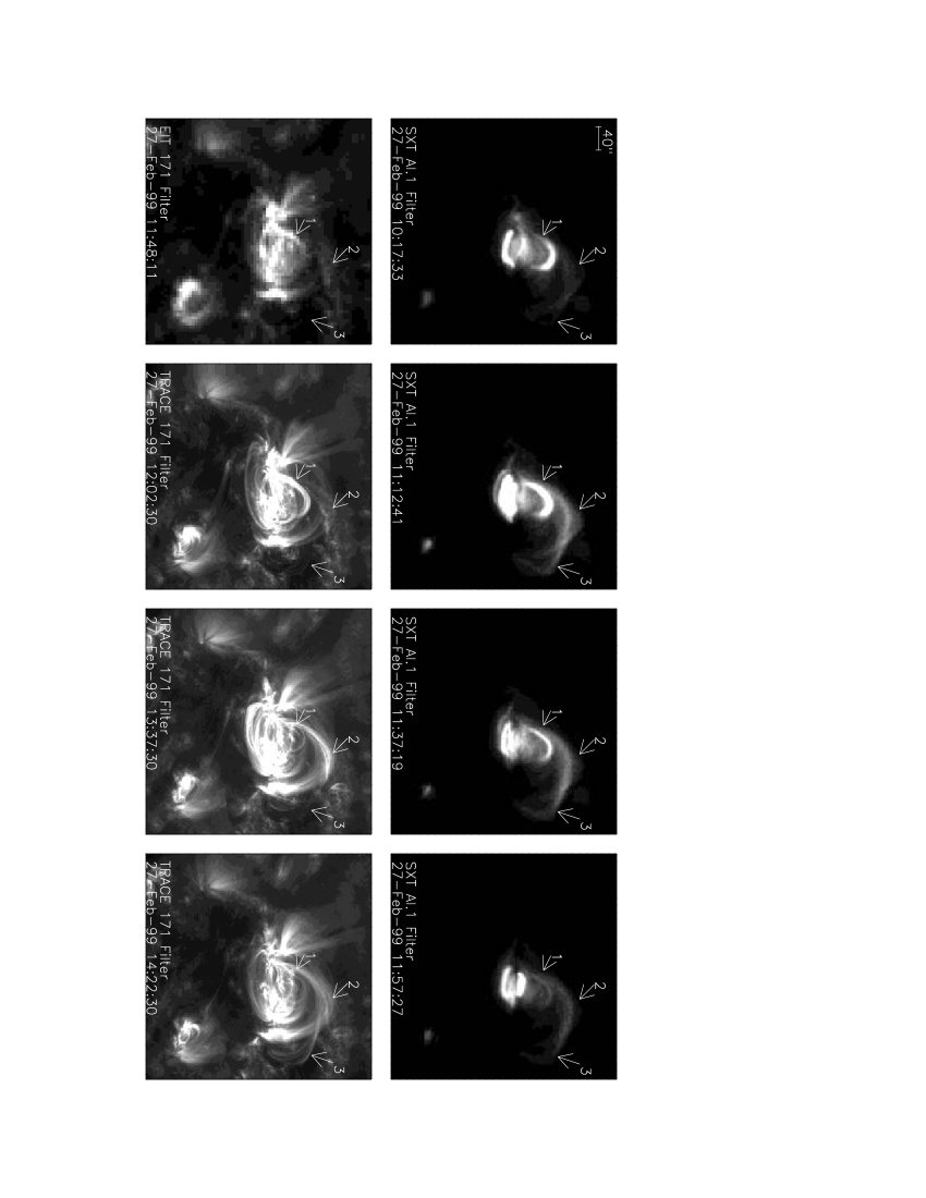
Figure 1: The evolution of three loops is shown with sample SXT Al.1 filter images, an EIT 171 Å filter image, and TRACE 171 Å filter images. All images are scaled linearly and all images from the same filter are scaled the same.

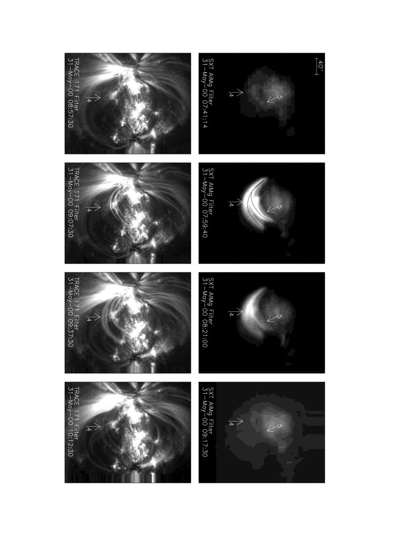
Figure 2: The evolution of two loops is shown with sample SXT AlMg filter images and TRACE 171 Å images. All images are scaled linearly and all images from the same filter are scaled the same.

Five distinct loops were visually identified in the SXT filter images of the active regions. On 1999 February 27, Loops 1, 2 and 3, shown in Figure 1, can be identified in the 10:17 UT SXT image (the last image available from that orbit) but are substantially brighter at 11:12 UT. It appears that Loop 1 changes orientation slightly between the 10:17 UT image and 11:12 UT image. It is unclear if it is the same loop or a different loop in the same location. The loops have dimmed in SXT by 11:57 UT and are completely absent from images taken in the next Yohkoh orbit. Loop 1 may be brightening in the EIT 11:48 UT image and is definitely bright in the first TRACE image of the active region at 12:02 UT. The two remaining loops brighten in TRACE substantially later. On 2000 May 31, Loops 4 and 5, shown in Figure 2, are absent in the 7:41 UT SXT image, but bright by 7:59 UT. The loops fade from SXT sometime between 8:21 and 9:17 UT during the Yohkoh eclipse. These loops begin to appear in the TRACE filter images at 9:07 UT and are gone by 10:12 UT. The projected lengths of these loops and the Gaussian widths of fits to the SXT loop intensity ($\sigma$) are given in Table 1.

In the SXT images, all of the loops appear to be monolithic structures. For instance, consider Loop 1 shown in Figure 3. SXT and TRACE images of Loop 1 are shown in the left panels. The section of Loop 1 within the envelope and between the cross lines is extracted and background subtracted using the method discussed in Winebarger et al. (2003b). The cut out from the SXT Al.1 image taken at 11:12 UT is shown along with a line plot of intensity averaged along the loop. All other images and line plots are taken from TRACE images. The SXT intensity was fit with a Gaussian (shown with a dashed line). The same Gaussian function, scaled to be consistent with the TRACE intensities is shown in all other line plots. The Gaussian width of the SXT loop is 1.7 SXT pixels or 4.2^′′. TRACE resolves several loops within what appears to be a single loop in the SXT data. We fit the TRACE intensities at each time with multiple Gaussian functions (shown with dash-dot lines); the Gaussian widths of the resulting fits in TRACE pixels are given in the figure. The smallest measured width was 4.0 TRACE pixels or 2.0^′′. Most of the loops, however, are blended and difficult to distinguish individually in single frames or to track from frame to frame.

A similar treatment of Loop 5 is shown in Figure 4. Again, Loop 5 appears to be a single loop in the SXT image with a Gaussian width of 1.5 SXT pixels, while TRACE resolves multiple structures. The three TRACE images at 9:02, 9:07 and 9:12 UT, however, all image the evolution of three distinguishable loops contained in the envelope of the SXT loop. The smallest Gaussian width of these loops is 2.9 TRACE pixels. After the data gap between 9:12 and 9:37 UT, it is unclear if those same loops exist or if TRACE is imaging other loops.

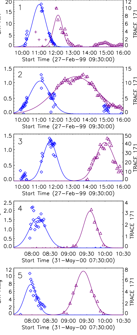
Figure 5: The SXT Al.1 or AlMg filter intensities are shown as diamonds and are in blue. The TRACE 171 Å intensities are shown as triangles and are in purple. The EIT data points are shown as crosses (only in Loop 1). The Gaussian fits to the lightcurves are shown as solid lines. The units of the SXT intensities are $10^{3}$ DN s^-1and the units of the TRACE intensities are 10 DN s^-1.

We extracted regions of the five loops and subtracted the background. We chose the regions of the loops that were most secluded from other bright structures to aid in background subtraction. The extracted regions of Loops 1 and 5 are shown in Figure 3 and 4. Regions of similar size were selected for Loops 2, 3, and 4. We computed lightcurves for each filter and each loop by averaging the data along the loop within the selected region and summing the data across the loop similar to the method discussed in Winebarger et al. (2003b) resulting in the DN s^-1 for each loop as a function of time. The SXT Al.1 filter and TRACE 171 Å filter lightcurves for the three loops in AR 8471 and the SXT AlMg filter and TRACE 171 Å filter lightcurves for the two loops in AR 9017 are shown in Figure 5. For Loop 1, additional points were added to the lightcurve before 12:00 UT by extracting the same region from aligned EIT data and scaling the measured intensities to match the TRACE 171 Å intensities at the 12:00 time. The lightcurves were fit with Gaussian functions, shown as solid lines. Note that because of the data gaps and the absence of TRACE data before 12:00 UT on 1999 Feb 27, the fits to the lightcurves are not well constrained and the information derived from them (the delay and lifetime) are approximations. The delay between the peak of the lightcurves in the two filters is approximately 67 minutes for Loop 1, 130 minutes for Loop 2, 200 minutes for Loop 3, 86 minutes for Loop 4 and 86 minutes for Loop 5. The lifetimes of the loops in each filter are assumed to be the full width half maximum of the fits and are given in Table 1.

Figure 5 and Table 1 give information on the lightcurves in the most sampled SXT filters. In Table 2, we give the maximum intensities of the loops in all available filters. These values represent the maximum observed values and are not based on a fit. We give these numbers in two separate ways. The first is the intensity summed across the loop, represented as $I_{filter}^{total}$. These values are what is plotted in Figure 5 and are compatible with our previous analysis (Winebarger et al. 2003b). We also provide this total value divided by $\sqrt{2\pi}\sigma$ where $\sigma$ is the width of the loop in either TRACE or SXT pixels found from the SXT filter images and given in Table 1. This value provides an estimate of the typical observed countrates per instrument pixel of the loop. For instance, the typical countrates for Loop 1 go from 4,200 DN s^-1 pixel^-1 in the SXT Al.1 filter images to 4.7 DN s^-1 pixel^-1 in TRACE 171 Å filter images. Loop 1 is also fairly bright in the SXT Be filter images.

While the range of typical TRACE intensities is relatively narrow (1.7-4.7 DN s^-1pixel^-1), the range of SXT filter intensities is quite broad (230-5,100 DN s^-1pixel^-1 in the SXT Al.1 filter). Furthermore, there is little correlation between the TRACE 171 Å intensities and the SXT intensities. For instance, Loops 1 and 2 and Loops 4 and 5 both have approximately the same intensity in the TRACE 171 Å filter, but have an order of magnitude difference in intensity in both the SXT filters. Loops 2 and 3 have approximately the same intensities in the SXT Al.1 filter, but there is a factor of 2 difference in their TRACE intensities. There is also little correlation between the delay of the appearance of the loop in the different filters (given in Table 1) and the intensities. Loops 4 and 5 have the same delay, but significantly different intensities in the SXT filters. There is a correlation between the intensity of the loop in the hotter SXT filters (Be or thick Al) and the ratio of the intensities in the cooler SXT filter to the TRACE 171 Å filter.

3 Discussion

In this paper, we have shown the evolution of five cooling loops. These loops first appear bright in SXT filter images (sensitive to plasma $>2.5$ MK) and then appear bright in TRACE filter images (sensitive to plasma $\sim 1$ MK). All loops appear as single, “monolithic” structures in the SXT images with Gaussian widths on the order of the resolution of the SXT instrument. These loops are resolved into several loops, each evolving independently, by TRACE. The widths of the TRACE loops are at least 3 TRACE pixels. These observations are qualitatively consistent with the predictions of the Impulsively Heated Multiple Strand Model.

The fact that there is no correlation between the brightness of the loops in SXT and TRACE filters demonstrates the non-linearity of the physics driving the plasma properties. It is impossible to say that a bright loop in TRACE must have been preceded by a bright loop in SXT or vice versa. Instead the evolution of the loops depends on the loop length, energy input, elemental abundances of the plasma, etc. Ideally, to understand better the evolution of these loops, we would use hydrodynamic models of each loop’s length and attempt to match the observed lightcurves exactly. Problems with the current data set such as the long data gaps caused by the Yohkoh orbit make quantitative modeling difficult. Furthermore, we were not able to resolve the loop length and geometry. The loop lengths were not well constrained by the geometric arguments used in previous analysis (see Winebarger et al. 2003b). It is difficult to make a conclusive statement concerning the correlation between the intensity of the loop in the hotter SXT filters and the ratio of the intensity in the cooler SXT filter to the TRACE 171 Å filter. It may be an important metric to aid in quantitative models.

Nitta (2000) and Schmieder et al. (2004) have examined SXT and TRACE active region observations for evidence of cooling loops. Though they observed that some loops would brighten in TRACE images in similar locations to where loops had previously brightened in SXT images, they concluded they were different loops due to the positional shifts. The five loops presented in this paper appear to shift as well. Figure 6 shows the relative positions of Loops 1, 2 and 3 determined from the TRACE data (solid lines) and SXT data (dashed lines) on a magnetogram from the Michelson Doppler Imager (MDI) flown aboard SOHO. The positions of the loops were found by “clicking on” the loop in the different images. The positions of the loops are most uncertain near the footpoints. In the TRACE images, many bright structures obscure the loops near the footpoints while the SXT filters are only sensitive to coronal plasma and hence do not image the true footpoint of the loop. The alignment of the images, which we believe is good to 10^′′, cannot account for all the differences in the coronal part of the loops’ positions. Magnetic field changes could account for the shift in position, similar to the magnetic motions observed during solar flares (e.g., Forbes & Acton 1996).

The IHMS model is similar to the scenario of energy release during solar flares. During large solar flares, however, the loops brighten in a systematic way, as the magnetic field sweeps through the reconnection region. Images of Loops 1 and 5 shown in Figures 3 and 4, however, show that there is no systematic way in which the loops within the bundle brighten. Though the IHMS model is motivated by the magnetic reconnection models, it does not exclude other impulsive heating models where strands within a loop are heated sequentially. For instance, Ofman et al. (1998) suggests that the heating due to resonant absorption of Alfvén waves has similar spatial and temporal characteristics as predicted by the IHMS model.

We demonstrate that what appears to be single loop in SXT images is actually a bundle of loops. Some of the individual loops in TRACE appear to be resolved, such as the three loops comprising “Loop 5” at 9:02, 9:07, and 9:12 UT shown in Figure 4 because their measured width exceeds the resolution of the TRACE instruments (2 pixels). Most of the loops, though, are blended together and difficult to distinguish. In a future investigation, we will determine if the individual loops within the bundle observed with TRACE are consistent with single temperatures and densities and hence are monolithic strands or if they, too, must contain a bundle of strands to explain their properties.

This paper has addressed moderate length active region loops that are completely visible (footpoint to apex) in EUV images (see Aschwanden et al. 2000 for a description of a large sample of these loops). It does not address other types of active region loops, such as the extended “fan” structures at the edges of active regions which are only visible in the EUV near their footpoints or the short, hot loops in active region cores that are bright in X-ray images and whose footpoints form the bright reticulated pattern called “moss” in EUV data. Antiochos et al. (2003) argue that the the moss loops must be heated steadily because the loops remain bright in X-ray images and never appear to cool through EUV images. Cargill & Klimchuk (2004) suggests that the heating is dynamic, but that multiple heating events within a strand keep the plasma at hotter temperatures. If future studies of these other structures confirm that the temporal characteristics of the energy deposition is markedly different than suggested by the IHMS model, it could imply that there are multiple mechanisms that release energy into the corona.

Table 1: Loop information.

Loop	Date	AR Number	Length	$\sigma$	Delay	FWHM - SXT	FWHM - TRACE
			(Mm)	(arcsec)	(minutes)	(minutes)	(minutes)
1	1999 Feb 27	8471	79	4.2	67	54	38
2	1999 Feb 27	8471	178	5.4	127	83	182
3	1999 Feb 27	8471	190	5.1	196	59	78
4	2000 May 31	9017	109	3.9	86	34	25
5	2000 May 31	9017	98	3.9	86	24	31

Table 2: Lightcurve information.

Loop	$I_{Be}^{total}$	$I_{Be}^{pix}$	$I_{Al12}^{total}$	$I_{Al12}^{pix}$	$I_{AlMg}^{total}$	$I_{AlMg}^{pix}$	$I_{Al.1}^{total}$	$I_{Al.1}^{pix}$	$I_{171}^{total}$	$I_{171}^{pix}$
1	$150$	$35$			$9,300$	$2,200$	$18,000$	$4,200$	$99$	4.7
2	$10$	$1.9$			$720$	$130$	$1,200$	$230$	$130$	4.7
3	$40$	7.7			$620$	$120$	$1,400$	$260$	$46$	1.8
4			170	43	$2,200$	$540$	$3,600$	$890$	$33$	1.7
5			730	180	$11,000$	$2,600$	$21,000$	$5,100$	$50$	2.6

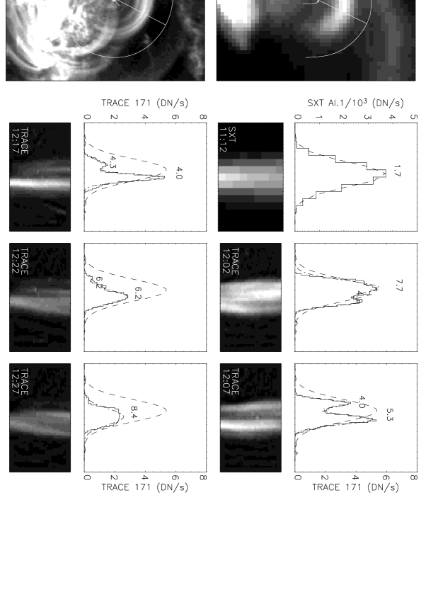
Figure 3: SXT Al.1 filter and TRACE 171 Å filter images of Loop 1 are shown on the left. The evolution of the area of the loop within the envelope and between the cross lines is shown in the smaller images. The line plots show the intensity summed along the loop.

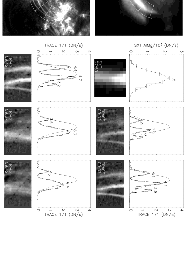
Figure 4: SXT AlMg filter and TRACE 171 Å filter images of Loop 5 are shown on the left. The evolution of the area of the loop within the envelope and between the cross lines is shown in the smaller images. The line plots show the intensity summed along the loop.

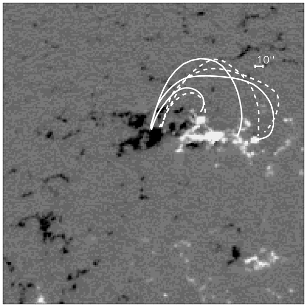
Figure 6: The relative positions of Loops 1, 2, and 3 determined from TRACE (solid) and SXT (dashed) images shown on a magnetogram from MDI.

References

- Antiochos et al. (2003) Antiochos, S. K., Karpen, J. T., DeLuca, E. E., Golub, L., & Hamilton, P. 2003, ApJ, 590, 547
- Aschwanden et al. (2000) Aschwanden, M. J., Nightingale, R. W., & Alexander, D. 2000, ApJ, 541, 1059
- Aschwanden et al. (2001) Aschwanden, M. J., Schrijver, C. J., & Alexander, D. 2001, ApJ, 550, 1036
- Cargill & Klimchuk (1997) Cargill, P. J., & Klimchuk, J. A. 1997, ApJ, 478, 799
- Cargill & Klimchuk (2004) Cargill, P. J., & Klimchuk, J. A. 2004, ApJ, 605, 911
- Delaboudiniere et al. (1995) Delaboudiniere, J.-P., et al. 1995, Sol. Phys., 162, 291
- Forbes & Acton (1996) Forbes, T. G., & Acton, L. W. 1996, ApJ, 459, 330
- Golub et al. (1999) Golub, L., et al. 1999, Phys. Plasmas, 6, 2205
- Handy et al. (1999) Handy, B. N., et al. 1999, Sol. Phys., 187, 229
- Klimchuk & Porter (1995) Klimchuk, J. A., & Porter, L. J. 1995, Nature, 377, 131
- Nitta (2000) Nitta, N. 2000, Sol. Phys., 195, 123
- Ofman et al. (1998) Ofman, L. and Klimchuk, J. A. and Davila, J. M. 1998, ApJ, 493, 474
- Parker (1988) Parker, E. N. 1988, ApJ, 330, 474
- Schmelz et al. (2001) Schmelz, J. T., Scopes, R. T., Cirtain, J. W., Winter, H. D., & Allen, J. D. 2001, ApJ, 556, 896
- Schmieder et al. (2004) Schmieder, B., Rust, D. M., Georgoulis, M. K., Démoulin, P., & Bernasconi, P. N. 2004, ApJ, 601, 530
- Schrijver et al. (2004) Schrijver, C. J., Sandman, A. W., Aschwanden, M. J., & DeRosa, M. L. 2004, ApJ, 615, 512
- Schrijver et al. (1999) Schrijver, C. J., et al. 1999, Sol. Phys., 187, 261
- Tsuneta et al. (1991) Tsuneta, S., et al. 1991, Sol. Phys., 136, 37
- Warren et al. (2002) Warren, H. P., Winebarger, A. R., & Hamilton, P. S. 2002, ApJ, 579, L41
- Warren et al. (2003) Warren, H. P., Winebarger, A. R., & Mariska, J. T. 2003, ApJ, 593, 1174
- Winebarger & Warren (2004) Winebarger, A. R., & Warren, H. P. 2004, ApJ, 610, L129
- Winebarger et al. (2003a) Winebarger, A. R., Warren, H. P., & Mariska, J. T. 2003a, ApJ, 587, 439
- Winebarger et al. (2003b) Winebarger, A. R., Warren, H. P., & Seaton, D. B. 2003b, ApJ, 593, 1164
- Winebarger et al. (2002) Winebarger, A. R., Warren, H. P., van Ballegooijen, A., DeLuca, E. E., & Golub, L. 2002, ApJ, 567, L89