A simple model for the complex lag structure of microquasars

The phase lag structure between the hard and soft X-ray photons observed in GRS $1915$+$105$ and XTE J$1550$+$564$ has been said to be “complex” because the phase of the Quasi-Periodic Oscillation fundamental Fourier mode changes with time and because the even and odd harmonics signs behave differentely. From simultaneous X-ray and radio observations this seems to be related to the presence of a jet (level of radio emission). We propose a simple idea where a partial absorption of the signal can shift the phases of the Fourier modes and account for the phase lag reversal. We also briefly discuss a possible physical mechanism that could lead to such an absorption of the quasi-periodic oscillation modulation.

1 Introduction

RXTE has provided us with a better picture of the temporal behavior of X-ray binaries, using such techniques as Fourier Transform (FT), time lag and coherence computation. The time lag between the low-energy ($2$ - $5$ keV) and the high-energy ($5$ - $20$ kev) is generally associated with Inverse-Compton of soft photons producing hard photons. Most of the time, the high energy variability lags behind the low energy emission ; this is the so called “hard-lag”. Surprisingly, there exist some observations where the QPO hard lags appear to change sign (becoming what is called a “soft-lag”) during an observation and also between observations. This is inconsistent with the Inverse-Compton explanation. In GRS $1915$+$105$ (e.g. Cui, 1999, Lin et al., 2000) and XTE J$1550$-$564$ (e.g. Wijnands et al., 1999, Cui et al., 2000), this unusual time lag behavior has been reported during outburst and/or the radio-loud state. Namely, the sign of the QPO’s time lag changed over a single observation whereas the sign of its first harmonics’ time lag stayed the same.

In their 1999 paper, Wijnands et al. point out that a change in the waveform of the QPO between the low and high energy emission could explain the sign difference in the lag of the fundamental and the first harmonic, but this was not explored further. Lin et al. (2000) noted that the presence of that same sign difference does not imply a real time delay. For example the same effect appears in the presence of a decaying oscillating signal. Here we will explore in more detail what is at the origin of the fundamental lag’s sign change. The same mechanism will also create the sign difference mentioned above without implying a real time delay.

Sect. $2$ discuss simultaneous radio and X-ray data from GRS $1915$+$105$ taken from the plateau/hard-steady ($\chi$, Belloni et al., 2000) state Muno et al (2001). We use this data to gain insight into the relation between radio/jet and the X-ray timing properties of the system. In Sect. $3$ we show the behavior of the Fourier Transform (FT) in the case of an absorbed sinusoid. In Sect. $4$ we make use of this simple, zeroth order, model to explain the complex lag structure observed in GRS $1915$+$105$ and XTE J$1550$-$564$ and see what we can infer about those systems.

2 The Case of GRS $1915$+$105$

Muno et al. (2001) studied the hard state ($\chi$ state in the classifications by Belloni et al., 2000, or radio plateau) using simultaneous X-ray and radio observations. In this section we will discuss Fig. $7$ and $8$ in Muno et al. (2001), in order to emphasize the observational constraints on the behaviour we are trying to explain here.

The left of their Fig. $8$ shows how the temporal properties (QPO frequency on the top and phase lag at the QPO frequency at the bottom) correlate with the different components of the X-ray flux, namely from left to right, the total flux, the thermal/disk flux and the power-law flux. By looking carefully at the plots two populations can be distinguished (the triangle and the cross). This distinction is more apparent in the graph showing the lag.

On the left upper panel of Fig. $8$ we see that for a QPO frequency higher than about two hertz, the QPO frequency appears to be correlated with the total flux and the power-law flux (which in fact dominates the total flux). This applies for most of the low-mass X-ray binaries. For a QPO frequency lower than $2$Hz, this QPO frequency no longer correlates with any of the X-ray fluxes. In fact all of the frequencies below $2$ Hz appear at a similar flux level for both the thermal and power-law flux, .i.e the cluster of triangles is very narrow. These points are also the ones with a high radio flux (the triangles represent the radio-loud state) as is seen in Fig. $7$. These radio-loud points are also the only ones to exhibit a positive phase lag. Concerning this lag, there is also another difference besides the change of sign between the radio-loud and the radio-quiet state: If we look at the left lower panel of Fig. $8$, there is no correlation between the lag and any of the X-ray fluxes. However, depending on wherever the source is radio-loud or radio-quiet the “clusters” of points appear to be perpendicular to each other.

In the radio-loud case, the temporal behavior of the source is modified for quasi constant X-ray fluxes. These modifications are a function of the radio flux. On Fig. $7$ is shown the evolution of the temporal properties such as the QPO frequency, the phase lag, the coherence and the ratio of low-frequency power as a function of the radio flux at $15.2$ GHz. Once again the radio-loud and radio-quiet points are well separated. The separation occurs at a radio flux of about $60$ mJy.

By looking in more detail at the first plot (QPO frequency - radio flux) we see that a QPO frequency less than two hertz is always associated with a radio flux of more than $60$ mJy. These same QPOs have a positive phase lag and show much less coherence than the QPOs in the radio quiet state. Moreover, the phase lag which seems totally uncorrelated with the radio flux when it is less than $60$ mJy, appears to be correlated with the higher radio fluxes. In the graph of the ratio of low-frequency power as function of the radio flux the possible correlation seems to reverse during the transition between radio-quiet and radio-loud.

Either these QPOs (less than $2$Hz, more than $2$Hz) arise from a different mechanism ( e.g. one related with the jet and the other one not) or there is a threshold in radio flux above which new phenomena appear in addition to the QPO mechanism. This could cause a modification of the temporal behavior of the source, especially relevant to the lag which seems to become proportional to the radio flux. We will focus on this last possibility. The presence of two different unrelated mechanisms, one from the jet and the other from the disk, seems improbable because of the smooth transition in QPO properties as a function of time (see for example Fig. $6$ of Muno et al, 2001) However, before exploring the possible origin for the change in temporal properties, we will look at the lag definition and its computation through Fourier transforms.

3 Fourier Transform and phase lag

3.1 Definition of lag and coherence

We will briefly go over the definition of the lag as presented by Vaughan & Nowak (1997). Suppose that $x_{1}(t_{k})$ and $x_{2}(t_{k})$ represent the X-ray flux in two energy bands (soft and hard) at time $t_{k}$. We note $X_{1}(\nu_{j})$ and $X_{2}(\nu_{j})$ as their Fourier transforms at the frequency $\nu_{j}$:

$$X(\nu_{j})=\frac{1}{2\pi}\int x(t_{k})e^{-i\nu_{j}t_{k}}dt_{k}$$

The time lag between the hard and soft X-ray is then defined as:

$$\delta t(\nu_{j})=\frac{1}{2\pi\nu_{j}}\times arg(X_{1}^{\star}(\nu_{j})X_{2}(\nu_{j}))\\ =\frac{arg(X_{2})-arg(X_{1})}{2\pi\nu_{j}}$$

Modification of one of the two phases (lowering the phase of the soft band or increasing the phase of the hard band) could induce the lag to change sign. More generally, any change in the phase of one of the bands, caused by internal or external phenomena, could lead to a sign change in the lag.

The coherence is a measure of how much of a signal $f$ can be predicted knowing a signal $h$. In our case it means how much of the high energy flux can be predicted knowing the low energy flux. If the two signals are related then the coherence is high; the maximum equals one, which correspond to the case where there is a linear transformation to go from one to the other.

3.2 Lag: a simple derivation

One can reproduce the observed behavior of the lag and harmonics using simple assumptions about the initial profile. The idea is to compare the Fourier representation of an initial profile (here a constant plus a cosine) taken to be the hard X-ray, to a modified profile taken to be the soft X-ray. We will then compute the lag between them and show a simple way to match the observed lag behavior.

If we compute the Fourier Transform of a sinusoid function we obtain the frequency, amplitude and phase. In order to make it similar to data we take the sinusoidal profile surimposed on a constant background and add a small amount of random noise to it. By using the FT we still find the frequency, amplitude and phase. Now take into account the case where some part of the modulated emission does not arrive to the observer but a part of it is ”absorbed/obscured” by a media located in the system. This would make a profile similar to the one of fig 1.

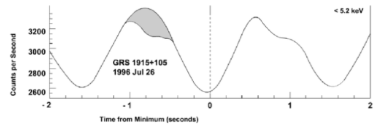
Figure 1: Morgan et al (1997) studied GRS $1915$+$105$ timing variability using average QPO-folded profile for the $0.63$Hz QPO. The profile show an absorbed-like feature for the soft energy band ($<5.2$ keV) emphasized on the figure by the grey ”missing part”. Morgan et al (1997) also showed the QPO profile at higher (hard) energies. For higher energies, the profiles appear more sinusoidal, i.e. the “missing/absorb part” becomes smaller.

Table $1$ shows the Fourier Transform using an input profile of unity plus a sinusoid with rms amplitude $rms=0.14$ minus a Gaussian profile of amplitude $\gamma$ centered to reproduce a profile like the one from the Fig. $15$ of Morgan et al (1997). The first line is the representation of the initial state, the test # 1 shows the first two frequencies of the Fourier representation of the absorbed signal.

Table 1: Representation obtained from the FT of a signal $1+\cos\phi$ plus an absorption of amplitude $\gamma$.

test	$\gamma$	freq	amp	phase
# 0	$0$	$1$	$0.14$	$0$
# 1	$0.07$	$1$	$0.12$	$-0.02$
	$0.07$	$2$	$0.016$	$1.27$

We see that by doing the FT on this signal we obtain different parameters for the sinusoid. Depending on the amount of ”absorption” we can obtain a smaller value for the amplitudes but the striking feature is the effect on the phase: a change is observed. Moreover, the sign of the phase difference is not the same for the fundamental and its first harmonics. If we take the formula for phase lag and say that only the low energy/soft X-rays are absorbed and not the hard ones we can compute the phase lag which appears as a consequence of the absorption of only part of the signal. Doing so reproduces the observed phase characteristics: a different sign for the fundamental and first harmonics. In addition, if the absorption is turned on, it creates a change in the sign of the lag. This comes from the fact that the FT adjusts the data with a shifted sinusoid, creating a phase difference. We propose that this is the origin of the changing sign of the lag presented in the previous section. This will also decrease the coherence between the two bands as a new signal is added to only one band. This happens without changing the primary physical phenomena that produces the emission in the two bands. The above results can be easily illustrated even using two sinusoidal signals with a $\pi/2$ phase between them:

$$\cos\theta+\epsilon\ \sin\theta=\frac{1}{\cos\phi}\ \cos(\theta-\phi),\tan\phi=\epsilon$$ (1)

The presence of a second, small, sinusoidal signal with a phase lag of $\pi/2$ and an amplitude $\epsilon$ is enough to create an “apparent” phase lag of $\phi$= atan$(\epsilon)$, which is about $\epsilon$, the amplitude of the perturbation.

If we now add the presence of a small harmonic to the QPO (of amplitude label $rms2$ in table $2$) and compare the result from the FT to that with the the same signal absorbed, the effect on the phase is even more striking. Table $2$ shows the results of such a simulation. Indeed, the induced phase lag between the real data and the absorbed one does not have the same sign at the fundamental vs. the first harmonics. This could be at the origin of the observed phenomena. In this work we show that an absorption of the low energy part of the signal will give the sign difference in the lag and also explain the observed change of sign for the fundamental.

Table 2: Representation obtain from the FT of a signal $1+\cos\phi+rms2\cos(2\phi)$ plus an absorption of amplitude $\gamma$.

test	rms2	$\gamma$	freq	amp	phase	lag
# 2	$0.07$	$0.0$	$1$	$0.14$	$0$
	$0.07$	$0.0$	$2$	$0.07$	$-\pi/2$
# 3	$0.07$	$0.07$	$1$	$0.12$	$-0.02$	0.02
	$0.07$	$0.07$	$2$	$0.054$	$-1.47$	-0.1
# 4	$0.07$	$0.1$	$1$	$0.112$	$-0.03$	0.03
	$0.07$	$0.1$	$2$	$0.048$	$-1.42$	-0.15

4 Application to microquasar observations

Using the above argument it appears that the use of an FT can lead to an incorrect interpretation of the lag in the presence of an absorption which depends on the energy band. To use this idea for the observations of GRS $1915$+$105$ presented in Sect. $2$, we need to find what may produce the ”absorbed” part of the QPO modulation. This has to be related to the jet, either having the same origin, or being a consequence of it. In the following we will assume that the QPO modulation is created by a hot spiral/point, for example in Varnière et al. (2002, 2005 in preparation) , and we are just interested in further absorption/modulation of this already existing modulation. As mentioned before, we choose to keep the same mechanism for the QPO above and below $2$Hz. Another possibility is that the QPO above $2$Hz comes from the disk while the one below $2$Hz is coming from the jet. This however, seems improbable because the passage through $2$Hz is smooth in all variables (see Fig. $6$ of Muno et al (2001).

Suppose that the basis of the jet/corona gets ”between” the observer and the spiral during one orbit of the spiral in the disk. This is enough to ”absorb” a part of the flux modulation, especially if it happens when the spiral is ”behind” the black hole and therefore near the maximum of the modulation. This simple model is able to explain both the occurrence of changing sign lag and its relation with the jet. In the same way it can also explain the fact that absorption is energy dependant, which makes the coherence drop. In fact, anything located inside the inner radius of the disk that can absorb a small part of the flux coming from the hot spiral could explain the changing sign of the lag and the complex behavior of the harmonics. But this needs to be related to the radio flux and therefore to the jet mechanism.

The first way to check this idea is to look at the QPO profile and see if there is an energy dependant departure from a sinusoidal signal. Morgan et al. (1997) show for the low-frequency QPO that there is indeed a departure from a sinusoid, which seems compatible with an absorption feature. This kind of analysis is difficult and rarely done for QPOs because of the lack of photons at these timescales. Another way to check the same properties is to see how the value of the lag depends on the energy band chosen. Using the idea of an energy dependant absorption we see that the negative lag will be more important between the lower energy band (say, $2-4$keV) and the highest possible band available, than between two high energy bands. It seems possible to have a change of the sign of the lag if we look to high enough energies (for example using INTEGRAL data).

This simple model can also be used with observational data to gain insight into the geometry near the black hole. The pulse shape of the QPO in different energy bands can allow us to constrain the relative geometry of the absorption region with respect to the emissive region (QPO origin), and also the column density of the absorber. We will test several mechanisms that could lead to this “absorbed-like” profile and compare them with observationnal data.

5 Conclusions

This letter shows how absorption can modify the X-Ray signal and give rise to an apparent change in the phase lag between the hard and soft photons. The model is phenomenological, and future simulation work is needed to yield more quantitive predictions that can be compared with observational data and thereby giving access to the geometry in the inner part of the disk. Indeed, with numerical simulation we intend to probe the relative geometry of the QPO emission region with respect to the absorbing media by using the shape of the QPO pulse. The use of RXTE and INTEGRAL data together with numerical simulations of the absorption of a “hot-spot” orbiting in the disk will further test this idea.