Absence of linear polarization in H$\alpha$ emission of solar flares

High sensitivity observations of H$\alpha$ polarization of 30 flares of different sizes and disk positions are reported. Both filter and spectrographic techniques have been used. The ZIMPOL system eliminates spurious polarizations due to seeing and flat-field effects. We didn’t find any clear linear polarization signature above our sensitivity level which was usually better than 0.1%. The observations include an X17.1 flare with gamma-ray lines reported by the RHESSI satellite. These results cast serious doubts on previous claims of linear polarization at the one percent level and more, attributed to impact polarization. The absence of linear polarization limits the anisotropy of energetic protons in the H$\alpha$ emitting region. The likely causes are isotropization by collisions with neutrals in the chromosphere and defocusing by the converging magnetic field.

1 Introduction

Linear polarization of the H$\alpha$ line emission of solar flares has been reported in numerous papers of the past. Hénoux & Chambe (1990) and Hénoux et al. (1990) made pioneering contributions. Metcalf et al. (1992, 1994) and Vogt & Hénoux (1999) found flare polarization with imaging spectrographs, and in the latter work a correlation in time with soft X-ray emission was reported. Vogt, Sahal-Bréchot, & Hénoux (2002) measured linear polarization of 3–5% in H$\alpha$ and H$\beta$ spectral observations of flare kernels. Firstova et al. (1994) observed up to 20% linear polarization at the Baikal Solar Vacuum Telescope. Kashapova (2003) reported also observations of linear polarization measured in moustaches or Ellerman bombs. Regular observations of impact polarization are made at the Ondrejov Observatory (Hénoux & Karlický 2003). Hanaoka (2003) has recently recorded linear polarization with high cadence and spatial resolution in a flare near disk center. He finds values above the half percent level in most of the regions of H$\alpha$ emission. The direction of linear polarization is preferentially perpendicular to the flare ribbons, and the polarization degree increases with H$\alpha$ brightness. Direction and degree happen to be well correlated also with the spatial gradient of the H$\alpha$ emission (Figs. 3 and 4 of Hanaoka 2003). As the total H$\alpha$ flare emission correlates well with soft X-rays, the correlation in time between the degree of polarization and H$\alpha$ brightness is consistent with the observations of Vogt & Hénoux (1999).

Impact polarization by precipitating flare particles has been the preferred interpretation since the early observations. As the observed linear polarization appears to peak in the gradual flare phase and significant polarization was reported at times outside impulsive hard X-ray enhancements (Hénoux et al. 1990), electrons were excluded. Fletcher & Brown (1995) exclude electrons also for theoretical reasons. Only flare accelerated ions may reach the level of H$\alpha$ emission in sufficient numbers. Thus beams of high-energy protons were proposed already by the first observers. As protons with energy below 350 keV are predicted to be most efficient in producing impact polarization (Vogt & Hénoux 1996), its measurement would yield unique information on protons accelerated in flares, a poorly known but possibly important flare constituent.

The measurement of linear polarization in the H$\alpha$ emission, however, is extremely difficult due to the presence of gradients in space and time. Spurious polarization signals can originate from limited seeing, differential optical aberrations and gain-table effects in CCDs. Whenever the gradients are large, which occurs near peak flare intensity, spurious polarization signals are the largest. Thus doubts about the reliability of the reported measurements of linear polarization have been raised (Canfield & Chang 1985; Fang et al. 1995).

A first set of imaging polarimetry measurements with higher sensitivity performed in Locarno revealed no polarization signal from H$\alpha$ emission in flares above the few tenths of a percent level (Bianda et al. 2003). The ZIMPOL (Zurich IMaging POLarimeter) instrument was used at the IRSOL facilities. The main advantage of ZIMPOL is that seeing and gain-table errors do not generate spurious polarization signals, which allows the system to achieve unprecedented polarimetric accuracy. Furthermore, the Gregory Coudé telescope at IRSOL has low instrumental polarization that is constant over the day. This combination allowed for a polarimetric accuracy and time resolution substantially better than in the measurements reported by other authors. In the first set of measurements performed at IRSOL (Bianda et al. 2003) it was not possible to observe a major flare event, and the H$\alpha$ filter allowed to study only the central part of the spectral line and not the behavior in the wings.

In the present paper we present new observations, including measurements taken with the spectrograph, in particular during the X17 flare on 28th October 2003.

2 Instrument and observations

ZIMPOL (Povel 1995; Gandorfer et al. 2004) allows to measure polarization with high modulation rate (84 kHz for linear, 42 kHz for circular), much higher than the typical seeing frequencies (which are below about 1 kHz). This eliminates seeing-to-polarization cross talk, which is one of the most important sources of spurious polarization signals in solar regions with high intensity gradients and rapidly evolving structures. The polarimeter is a single-beam system, and the same CCD pixels are used to measure all Stokes parameters. Instrumental spurious effects are thus minimized, and no flat-field technique is needed to obtain accurate polarization images.

The 45 cm aperture Gregory Coudé telescope in Locarno has a 200″ field of view. It is well suited for polarimetric observations, since instrumental polarization, mainly due to two folding mirrors, is low and depends only on the Sun’s declination. The effects of the two folding mirrors mutually cancel around the equinoxes, so the instrument is virtually polarization free (Wiehr 1971; Sánchez Almeida et al. 1991).

The polarimetric observations were obtained with two techniques: imaging with a narrow bandpass filter, and spectrography with the Czerny-Turner spectrograph.

In both cases, the ZIMPOL analyzer is the first optical device placed after the exit of the telescope along the hour axis. It consists of a piezoelastic modulator and a polarizer, which can be rotated in order to choose the orientation of the linear polarization measurement. The set-up used allows to record simultaneously the intensity, one linear polarization component, and the circular polarization $V/I$. A Dove prism image rotator compensates for image rotation.

2.1 Two-dimensional spatial polarimetry

For spatial polarimetry observations, a 0.6Å FWHM H$\alpha$ filter is placed in front of the Dove prism. A beam splitter feeds two instruments: the Fachhochschule Wiesbaden (FHSW) flare detector system (Küveler et al. 2003) and the ZIMPOL CCD camera. Telecentric optics demagnifies the image on the sensors.

The most promising active area, where a flare is expected, is monitored. Priority is given to regions close to the limb, where the largest observable impact polarization is expected. The polarization optics is set in such a way that the linear polarization oriented parallel to the closest limb is measured as positive $Q/I$. Negative signatures are thus expected (Vogt & Hénoux 1996).

The FHSW flare detector system stores intensity images (12 per second) and reads the GPS signal to provide the precise time of the observation. Data are continuously stored in a buffer of programmable length (typically 5 minutes) as long as no events are detected. If the intensity exceeds a predefined threshold, the recording is triggered. Data in the buffer are then permanently stored together with the recordings of the following time interval of typically 15 minutes. The trigger signal is sent to ZIMPOL together with the precise GPS time information. The ZIMPOL software has been adapted to communicate with the FHSW system and to allow the data storage with the same buffer technique. ZIMPOL data are stored with a rate of typically one image every four seconds. Before or after a flare observation, calibration data and dark frames are recorded. In the resulting images one pixel subtends $1\arcsec\times 1\arcsec$.

2.2 Spectrographic mode

In the spectrographic mode the active regions are surveyed with the slit jaw plane viewer and the H$\alpha$ image of the guiding telescope. The spectrum is recorded by the ZIMPOL camera. The optical components are rotated in order to have the slit parallel to the closest limb of an active region and such that positive $Q/I$ is defined to be directed along the slit. When flare is visually detected, the telescope is moved in order to record data from the erupting area. The measurements of $Q/I$ and $U/I$ are obtained separately, rotating the analyzer by 45^∘. In some cases the complete Stokes vector, otherwise only $Q/I$ and $V/I$, were recorded.

2.3 Spurious signature sources

The known possible sources of spurious polarization have been examined. The instrumental polarization, which consists of a polarization offset and a cross talk between different Stokes components, can be easily compensated for in the data reduction process, since its variation over a day is negligible. Parasitic light could affect dark frames and introduce intensity-to-polarization cross talk and other spurious signatures. Some of our first observations were corrupted by this problem, which could be solved with better baffling. From other kinds of ZIMPOL measurements we know that very strong intensity gradients can introduce spurious signatures of order a few tenths of percent in the polarization images, and are seen only in a few of the pixels of the CCD. Another possible source of error could be related to the adjustments of the optical setup. Its correctness was verified in most observations by feeding a signal of known polarization into the system before the analyzer for a few seconds.

Some further tests were performed to check the ability of ZIMPOL to detect signatures evolving fast in time. Artificially modulated polarization signals inserted in front of the analyzer were correctly measured. Test recordings were made to obtain H$\alpha$ magnetograms of active regions by recording $V/I$ with the filter positioned in the blue and red wings as well as in the line core. The resulting circular polarization patterns were consistent with SOHO/MDI magnetograms.

3 Results

The observed 30 flares are summarized in Table 1, where we give the date, the GOES classification in soft X-rays, the time of maximum soft X-ray flux, the $\mu=\cos\theta$ position on the disk ($\mu$ noted as $<0.0$ means outside the disk), the noise level and the highest observed polarization value, the last two entries will be described later in more details. In contrast to the measurements reported by other authors, a clear impact polarization signal was never found.

Table 1: List of flare events observed. GOES flare classification (soft X-ray peak flux), position on the disk, and linear H$\alpha$ polarization noise and peak value are given.

Filter data
Date	Classi-	UT	$\mu$	Noise	Max
	fication	Max		level [%]	Pol. [%]
04 Jul 2002	C2.4	10:45	0.23	0.02	-
04 Jul 2002	C3.0	13:34	0.34	0.03	-
04 Jul 2002	C7.1	14:57	0.35	0.02	-
05 Jul 2002	M3.2	13:26	0.07	0.05	-
07 Jul 2002	SF	13:03	0.66	0.03	0.05
11 Jul 2002	C2.1	07:13	0.41	0.03	-
11 Jul 2002	C4.0	11:21	0.43	0.03	0.06
11 Jul 2002	C2.5	12:08	0.43	0.02	0.03
11 Jul 2002	M1.0	14:19	0.47	0.03	0.05
11 Jul 2002	M5.8	14:48	0.52	0.02	0.07
18 Jul 2002	X1.8	07:24	0.81	0.02	-
02 Aug 2002	M1.0	10:51	0.45	0.03	0.04
04 Aug 2002	C7.4	07:14	$<0.0$	0.07	-
04 Aug 2002	M6.6	10.33	$<0.0$	0.07	-
04 Nov 2003	C5.7	11:19	$<0.0$	0.04	-
04 Nov 2003	M1.1	13:45	$<0.0$	0.04	-
05 Nov 2003	M5.3	10:52	$<0.0$	0.11	-
18 Nov 2003	M3.9	08:31	0.96	0.02	-
19 Nov 2003	C8.8	08:17	1.0	0.02	0.03
Spectrograph observations
Date	Classi-	UT	$\mu$	Noise	Max
	fication	Max		level [%]	Pol. [%]
11 Jun 2003	C8.3	08:30	0.49	0.09	-
11 Jun 2003	M1.1	10:33	0.48	0.07	-
11 Jun 2003	M1.4	11:09	0.48	0.08	-
11 Jun 2003	M2.7	13:21	0.48	0.10	-
12 Jun 2003	C7.2	08:12	0.2	0.08	-
12 Jun 2003	C8.4	08:29	0.87	0.09	-
12 Jun 2003	C8.1	10:27	$<0.0$	0.40	-
12 Jun 2003	C7.1	11:47	0.2	0.08	-
12 Jun 2003	M1.0	14:03	$<0.0$	0.20	-
27 Oct 2003	M6.7	12:43	0.86	0.05	-
28 Oct 2003	X17.1	11:10	0.95	0.05	-

Figure 1 shows the evolution in time of the flare that occurred on 7th July 2002 at S19E46. The recordings started at 12:50 UT and terminated at 13:11 UT. A total of 320 exposures were taken every 4 seconds, each of them with 2 s integration time. Each square represents a solar disk area of $120\arcsec\times 110\arcsec$. The first and fourth row contain the H$\alpha$ intensity images, the second and fifth row $Q/I$, while the third and sixth row show $V/I$. The $Q/I$ and $V/I$ images have been obtained by averaging 10 subsequent exposures. The intensity image corresponds to a single exposure (in the the middle of the time interval). The only faint polarization signature that can be clearly detected is in $V/I$. It is due to the Zeeman effect at the position of a sunspot (dark feature in the $I$ images).

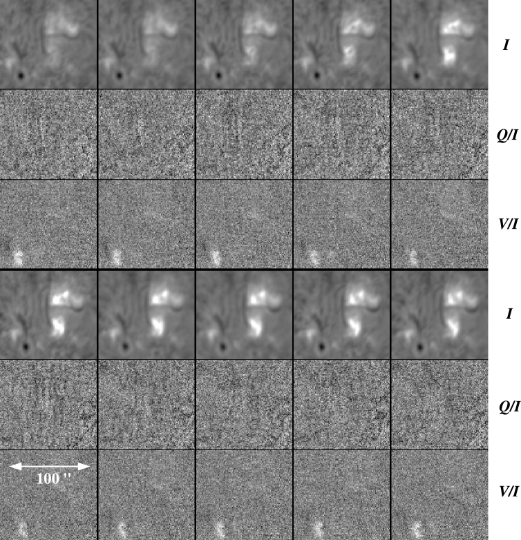
Figure 1: Images of three Stokes parameters during a flare on 7th July 2002. Time progresses from left to right in two minute steps and continues in the lower half.

Spatial Stokes profiles corresponding to a single row in the 6th set of images of Fig. 1 (bottom left) are shown in Fig. 2. The solid curves represent the profiles passing through the flare region, 44″ from the bottom of the image, while the dot-dashed curves correspond to profiles through the sunspot, 18″ from the bottom. The noise level (rms) of single $Q/I$ exposures (2 seconds) is around 0.4 %, similar to all other flare observations. The over 10 exposures averaged polarization profiles reported in Fig. 2 allow to detect a $V/I$ signature. The 0.3 % signal of the $V/I$ dot-dashed profile is a Zeeman signature of the sunspot, due to the fact that the filter is not perfectly centered in the H$\alpha$ line. Thus any signature that exceeds a few tenths of a percent is visually distinguished easily on the polarization images of Fig. 1.

Figure 2: Single spatial profiles taken from the 6th set of images of Figure 1. Horizontal rows are displayed passing through the flare region (solid line) and through the sunspot (dot-dashed line).

For all filter mode observation data a visual examination of the time evolution of the intensity and $Q/I$ frames is performed. Only in few flares we see small signatures. These are quite well related to intensity gradients and for this reason we suspect an instrumental origin. Strong signatures, clearly exceeding several 0.1 %, were never detected, but to give a measure of this results we proceed as follows. We choose for each event a $10\arcsec\times 10\arcsec$ area placed either where the intensity maximal value is detected or where we visually see suspect $Q/I$ signatures. The time evolution of the $Q/I$ values averaged over this area is analyzed. The rms is calculated and given for each event in Table 1 as noise level. We consider also the running average over ten exposures of $Q/I$ averaged over the small $10\arcsec\times 10\arcsec$ area, corresponding to an interval of 40 seconds. The largest absolute value is reported in Table 1 as maximal polarization value. Where this value is missing in Table 1 the measured maximal polarization signature is less than the reported noise level.

As example we describe the reduction of the 7th July 2002 flare. The $10\arcsec\times 10\arcsec$ area is centered at 65″ from the left and 40″ from the bottom of the images reported in Fig. 1. For each of the 320 frames we have the averaged values over the small area for intensity, linear and circular polarization, as reported in Fig. 3. The $Q/I$ evolution is almost unaffected by the flare event.

Figure 3: The time evolution of intensity, $Q/I$ and $V/I$ averaged over a small, 20″$\times$14″area in the flaring region shown in Fig. 1.

Also in the spectrograph measurements no significant signature could be detected, which could be interpreted as impact polarization. As an example we present an observation performed during one of the largest flares ever observed: the X17.1 flare of 28th October 2003. Figure 4 is a composite image of RHESSI and TRACE data, on which the positions of the slit in the different observations performed with ZIMPOL are drawn. The time intervals during which the event was observed at each position are given in Table 2. The soft X-ray phase, during which linear polarization has been claimed to be observed in other flares, lasted from 10:32 UT until beyond 13:00 UT. All of the slit positions except number 3 are traversing the soft X-ray source. The gamma ray emission with energy 0.8–7 MeV was enhanced from 10:34 until the end of the RHESSI observing time at 11:25 UT. Initial imaging results of the 2.2 MeV line emission integrated over 11:06-11:25 UT show two sources with a similar separation as seen in Fig. 4 for hard X-rays (Hurford et al. 2004). The centroid positions of the 2.2 MeV line are slightly shifted ($\sim 15$″ East, i.e. left in Fig. 4) relative to the hard X-ray centroids.

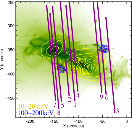
Figure 4: Positions of the spectrograph slit on the intensity maps recorded by TRACE (195 Å, gray scale) and RHESSI (contour lines) for the region of the X17.1 flare of 28th October 2003 taken at 11:11:53 UT. Soft X-ray contours are white, hard X-ray contours are black.

Table 2: Time intervals of the observations at the different slit positions shown in Fig. 4.

slit position	begin	end
1	11:10	11:20
2	11:22	11:25
3	11:26	11:29
4	11:31	11:33
5	11:34	11:36
6	11:37	11:39
7	11:42	11:44
8	12:02	12:03
9	12:07	12:08

Figure 5 shows the result of a 10 s measurement obtained at slit position 5 at 11:34 UT. The intensity image is corrected for flat field. The $Q/I$, $U/I$ and $V/I$ images are smoothed with the wavelet technique (Fligge & Solanki 1997). In the linear polarization images we find the usual symmetric Zeeman signatures in the atomic solar lines but not in the telluric lines. They can be seen as an expression of the polarimetric accuracy. In the H$\alpha$ line however, no signature is detectable that could indicate impact polarization. An increase of the noise due to low intensity can be noticed in the lower part of the H$\alpha$ line. Correlated with the strong intensity gradient in the bottom part of the flare region, a small signal below 0.3 %, probably of spurious origin, can be noticed (cf. Fig. 6). In the $V/I$ image the H$\alpha$ circular polarization changes sign in the flare emission region, in contrast to the surrounding absorption lines.

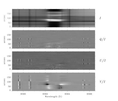
Figure 5: Full Stokes spectral images taken with the spectrograph slit in position 5 of Fig. 4.

Figure 6 shows spectral profiles extracted from Fig. 5 for two different spatial pixels. The solid lines correspond to the horizontal row at 59″ from the bottom, where the largest linear polarization signal in H$\alpha$ is detected. It includes the region with the largest intensity gradient. The dotted line refers to the position with maximum H$\alpha$ intensity (horizontal row at 77″).

Figure 6: Spectral Stokes profiles taken from two different horizontal rows of Fig. 5. A position with strong flare emission is shown dashed, while a quiet position is represented by the solid curves.

All other observations taken during this and the other measured flares give the same null results for impact polarization. Signals similar to those seen in the linear polarization in Fig. 6, which could be related to spurious signals as mentioned in Section 2.3, are detected in few cases in other spectrograph data. This signatures are correlated with the intensity gradient and thus have negative and positive signs that partially cancel when averaging. A rebinning of the spectral $Q/I$ images, averaging over $4\times 4$ pixel, cancels this spurious signatures. The rms of the $Q/I$ spectra is reported in Table 1 as noise level. These values are calculated in a 10 seconds exposure $Q/I$ measurements, the slit of the spectrograph was subtending 1.5″ and a pixel element (after rebinning) has a size of $5\arcsec\times 40$ mÅ. Large rms values are found when observing outside the disk.

4 Discussion

No linear polarization in H$\alpha$ has been found in our measurements of 30 solar flares from GOES class C2.1 to X17.1. These events were associated with hard X-ray emission when RHESSI was observing, one of them even in gamma-ray lines. Non-thermal electrons and possibly protons must have been accelerated in these flares, propagated to the chromosphere and impacted on hydrogen atoms. The question thus arises why impact polarization was not detected.

Impact polarization has been observed in the laboratory and agrees with calculations from first principles (Percival & Seaton 1958). For a review, the reader is referred to Vogt & Hénoux (1996). The degree of polarization $P$ depends on the viewing angle $\beta$ between the impacting particle’s velocity and the observer, and on the energy $E$ of the particle:

$$P(\beta,E)=bP_{90}(E)\,{\sin^{2}\beta\over{1-P_{90}(E)\cos^{2}\beta}}\ \ \ ,$$ (1)

where $P_{90}(E)$ is the polarization at $\beta=90^{\circ}$ for a fully collimated beam. The polarization peaks at a perpendicular viewing angle and vanishes for a parallel line of sight relative to the particle motion. Following Fletcher & Brown (1995) we take $P_{90}=0.246$ of 1 MeV protons (3p-2s transition). This value must be multiplied by the anisotropy factor $b<$1, ranging from 0 (fully isotropic), about 0.5 for a cosine-distribution in pitch angle, to 1 for a unidirectional beam (Hénoux et al. 1983).

The interpretation of the previously reported alleged detections of linear polarization favored proton beams as the cause. This is consistent with reported evidence for flare accelerated protons. Nuclear excitation lines in gamma-rays are produced by high energy protons impinging on the chromosphere (Ramaty & Murphy 1987). In one of the flares reported here (Fig. 4), RHESSI has indeed recorded clear signatures of protons. Theoretical models based on proton fluxes consistent with such observations have been published by Vogt et al. (1997). They predict linear polarizations of a few percent, assuming a fully collimated proton beam.

The absence of an observable degree of linear polarization may have two reasons: (i) The energetic protons may not reach the atmospheric level of the H$\alpha$ emission in sufficient numbers, or (ii) the protons may be nearly isotropic when they reach that level.

The first possibility may be excluded in view of the moustache phenomenon. In certain large flares there is sometimes a phase when the H$\alpha$ line is broader than 10 Å. This suggests that individual hydrogen atoms move with velocities of more than $10^{7}$ km s^-1, as one may expect after collisions with energetic particles (Ding, Hénoux, & Fang 1998). We have therefore examined with special care the linear polarization for such events. One such case was presented in Sect. 3. The circumstance that no polarization above threshold was found suggests that the exciting particles (if present) were not beamed. This is consistent with the fact that the H$\alpha$ line profile is not broadened in only the red direction during the moustache phase.

In the models quoted above, the protons are assumed to be accelerated isotropically in the corona. A beam develops as protons propagating in the plasma are slowed down by electron friction (Hénoux et al. 1990). The loss of energy is proportional to the distance traveled. Protons propagating parallel to the guiding magnetic field travel the shortest distance, while the others follow a path that is a factor of $1/\cos\alpha$ longer, where $\alpha$ is the pitch angle between the proton velocity and the magnetic field. Obviously, the resulting beam is not strongly collimated, contrary to some models assumptions. Collimation is further limited by the beam instability to growing Alfvén waves. If the instability occurs, the protons become nearly isotropic and propagate parallel to the magnetic field with a mean velocity of the Alfvén speed (Wentzel 1974).

In addition, there are processes that work in the opposite direction, trying to randomize the angular distribution. For instance, interactions with neutrals scatter the protons efficiently. The scattering time $\tau$ of a proton with energy of 1 - 500 MeV in a weakly ionized gas is

$$\tau=-{E_{\rm MeV}\over{dE_{\rm MeV}\over dt}}\approx{E_{\rm MeV}^{2}\over 3\cdot 10^{-12}n_{H}\beta(\ln E_{\rm MeV}+22.3)}\ \ ,$$ (2)

where $E_{\rm MeV}$ is the kinetic proton energy in MeV and $n_{H}$ is the hydrogen density in cm^-3 (Benz & Gold 1971, after Hayakawa & Kitao 1956). With a $n_{H}\approx 6\cdot 10^{13}$cm^-3 in the H$\alpha$ emitting region, the mean free path for a proton of 1 MeV for example becomes 75 km. Thus collisional focusing is limited to the corona and the transition region, and works in the opposite sense in the chromosphere.

Isotropization is enhanced by a second effect based on conservation of the magnetic moment. Charged particles are forced into more transverse orbits as they propagate downward along a converging magnetic field. The pitch angle $\alpha$ is related to the local magnetic field $B$ by

$$\alpha={\rm arcsin}\left(\sin\alpha_{0}{\sqrt{B\over B_{0}}}\right)\ \ \ ,$$ (3)

where index 0 refers to a site of reference along the orbit or the initial value at the release from the acceleration region. The effect widens up a beam that has an initial pitch angle width of $\alpha_{0}^{\rm max}$ to $\alpha^{\rm max}$ at a place with magnetic field $B>B_{0}$ according to Eq.(3). Let the initial velocity distribution be

$$f_{0}(v,\alpha_{0})\ =\ f(v)H(\alpha^{\rm max}_{0}-\alpha_{0})\ \ \ ,$$ (4)

where $v$ is the absolute value of the velocity (which is conserved) and $H$ the Heaviside function. At the local magnetic field $B>B_{0}$ the pitch angle $\alpha$ is given by Eq.(3), and

$$f(v,\alpha)\ =\ f(v)H(\alpha^{\rm max}-\alpha){\cos\alpha\over\sqrt{(B/B_{0}-1)+\cos^{2}\alpha}}\ .$$ (5)

Thus an increase by a factor of 4 in the magnetic field strength from the acceleration site to the H$\alpha$ emitting region would enhance a small pitch angle by approximately a factor of 2 (Eq.3). The proton beam widens up in velocity space by the same factor. Scattering by neutrals and conservation of the magnetic moment may act together to reduce the anisotropy to a level where impact polarization becomes negligible.

Other causes for linear polarization by impact polarization at the one percent level have been proposed, such as by the downgoing heat flux (Hénoux et al. 1983), by evaporative upflows (Flechter & Brown 1998), and by return currents (Hénoux and Karlicky 2003). They apparently also overestimated the effect trying to match the previously reported values.

5 Conclusions

Linear polarization values up to 20% and more have been reported in the literature for more than 20 years. We have not been able to confirm these values with an imaging system that recognizes flares, registers both the preflare and flare phases at noise levels of some 0.1%. The fast polarization modulation and special instrumental precautions much reduce the level of spurious effects from seeing and instrumental causes compared to all previous observations.

Our data set includes 30 flares of great variety, varying from small to very large by two orders of magnitude in peak soft X-ray flux. They occurred at different positions on the disk, some near the limb or even beyond the disk. The observations were made with high time resolution and cover all the flare phases. We have used both imaging and spectrographic polarimetry.

None of flares showed more than 0.07% linear H$\alpha$ polarization in a $10\arcsec\times 10\arcsec$ area during an integration time of 40 seconds. The above peak value and all others are not significantly different from zero.

These observations do not exclude impact polarization in general, but contradict all previous positive reports. Our theoretical considerations demonstrate that the anisotropy of energetic ions at the site of H$\alpha$ emission has been largely overestimated in the past to interpret the previously reported polarization levels. Impact polarization may exist only if it is limited to a smaller area or shorter time. Future measurements of solar flare linear polarization may still be meaningful if done at the present noise level of some 0.1%, excluding seeing effects and instrumental polarization, and with enhanced spatial and temporal resolution.

- (1) Benz, A.O., Gold, T. 1971, Solar Phys., 21, 157
- (2) Bianda, M., Stenflo, J.O., Gandorfer, A. M., Gisler, D., Küveler, G. 2003, in: Solar Polarization 3, ASP Conf. Ser. 307, eds. J. Trujillo Bueno, Sánchez Almeida, p. 487
- (3) Canfield, R. C., Chang, C.-R. 1985, ApJ, 295, 275
- (4) Ding, M. D., Hénoux, J.-C., Fang, C. 1998, A&A, 332, 761
- (5) Fang, C., Feautrier, N., Hénoux, J.-C. 1995, A&A, 297, 854
- (6) Firstova, N.M.,& Boulatov, A.V. 1996, Solar Phys., 164, 361
- (7) Fletcher, L. & Brown, J.C. 1995, A&A, 294, 260
- (8) Fletcher, L. & Brown, J.C. 1998, A&A, 338, 737
- (9) Fligge M.,& Solanki S.K. 1997, Astron. Astrophys. Suppl. Ser., 124, 579
- (10) Gandorfer, A. M., Povel, H. P., Aebersold, F., Egger, U., Feller, A., Gisler, D., Hagenbuch, S., Steiner, P., Stenflo, J. O. 2004, A&A, 422, 703
- (11) Hayakawa, P., Kitao, K. 1956, Prog. Theor. Phys., 16, 139
- (12) Hanakoka, Y. 2003, ApJ, 596, 1347
- (13) Hénoux, J.-C., Chambe, G. 1990, J. Quant. Spectrosc. Radiat. Transfer, 44, 193
- (14) Hénoux, J.-C., Chambe, G., Tamres, D., Feautrier, N., Rovira, M., Sahal-Bréchot, S. 1990, ApJS, 73, 303
- (15) Hénoux, J.-C., Karlický, M. 2003, A&A, 407, 1103
- (16) Hurford, G. J., Krucker, S., Lin, R. P., Schwartz, R. A., Share, G. H., Smith, D. M. 2004, AAS meeting, 204, 2.02
- (17) Kashapova, L.K. 2003, in: Solar Polarization 3, ASP Conf. Ser. 307, eds. J. Trujillo Bueno, Sànchez Almeida, p. 474
- (18) Küveler G., Klein, R., & Bianda, M. 2003, Photonik, 2/2003, 66
- (19) Metcalf, T., Wulser, J.-P., Canfield, R. C., Hudson, H. 1992, in: The Comption Observatory Science Workshop, Vol. NASA Conf. Proceedings, 3137, 536
- (20) Metcalf, T., Mickey, D., Canfield, R., Wulser, J.-P. 1994, in : High Energy Solar Phenomena, Vol. AIP Conf. Proceedings, 294, 59
- (21) Percival, I.C., Seaton, M.J. 1958, Phil. Trans. Roy. Soc. London, Series A, 251, 113
- (22) Povel, H. 1995, Optical Engineering, 34, 1870
- (23) Ramaty, R., Murphy, R. J. 1987, Space Sci. Rev., 45, 213
- (24) Sánchez Almeida J., Martinez Pillet, V., & Wittmann, A.D. 1991, Solar Phys., 164, 361
- (25) Wentzel, D.G. 1974, Ann. Rev. Astr. Ap., 12, 71
- (26) Vogt, E., Hénoux, J.-C. 1996, Solar Phys., 164, 345
- (27) Vogt, E., Sahal-Bréchot, S., Hénoux, J.-C. 1997, A&A, 324, 1211
- (28) Vogt, E., Hénoux, J.-C. 1999, A&A, 349, 283
- (29) Vogt, E., Sahal-Bréchot, S., Hénoux, J.-C. 2002, in: Proceedings Second Solar Cycle and Space Weather Euroconf., ESA SP-477, 191
- (30) Wiehr, E. 1971, Solar Physics, 18, 226