Neural Networks as a Composition Diagnostic for Ultra-high Energy Cosmic Rays

Abstract

We analyze here the possibility of studying mass composition in the Auger data sample using neural networks as a diagnostic tool. Extensive air showers were simulated using the AIRES code, for the two hadronic interaction models in current use: QGSJet and Sibyll. Both, photon and hadron primaries were simulated and used to generate events. The output parameters from the ground array were simulated for the typical instrumental and environmental conditions at the Malargüe Auger site using the code SAMPLE. Besides photons, hydrogen, helium, carbon, oxygen, magnesium, silicon, calcium and iron nuclei were also simulated. We show that Principal Components Analysis alone is enough to separate individual photon from hadron events, but the same technique cannot be applied to the classification of hadronic events. The latter requires the use of a more robust diagnostic. We show that neural networks are potentially powerful enough to discriminate proton from iron events almost on an event-by-event basis. However, in the case of a more realistic multi-component mixture of primary nuclei, only a statistical estimate of the average mass can be reliably obtained. Although hybrid events are not explicitly simulated, we show that, whenever hybrid information in the form of $X_{max}$ is introduced in the training procedure of the neural networks, a considerable improvement can be achieved in mass discrimination analysis.

1 Introduction

The origin of ultra-high energy cosmic rays (UHECRs) is currently one of the most exciting problems in modern astrophysics. Up to now, no astrophysical object is known that could accelerate charged particles to such energies. Besides, if the sources are located on cosmological distances, then it would be expected that the Cosmic Rays arriving to the Earth would loose energy after interacting with the cosmic microwave background above an energy of about $6\times 10^{19}$ eV [1], the threshold for photo-pion production in interactions with the cosmic microwave background radiation (CMBR). This energy would therefore mark a sharp bend in the Cosmic Rays energy spectrum. Is is not clear at present whether such bent is seen by the experiments operating so far. If the sources are nearby, then an anisotropic distribution of arrival directions is expected because in this case the directions of arrival would point to the sources, and this does not seem to be the case either.

Alternative explanations of the existence of the UHECRs have been developed over the last few years. Indeed, a whole spectrum of models exists, ranging from the more conservative bottom-up models, in which nuclei are accelerated up to the highest observed energies [2], to the more radical top-down scenarios where either new particles or exotic phenomena are invoked to produce the particles at already higher energies than those measured ([3] for example).

The discrimination among these models, requires an accurate determination of the energy spectrum, the distribution of arrival directions and the identity of the particles.

Additionally, accuracy must be complemented with high statistics. During the next few years, it is expected that at least two major experiments will attain this requirements: Auger South and North [4] and the Extreme Universe Space Observatory, EUSO [5].

In this work will concentrate on the specific characteristics of the Auger experiment. Nevertheless, the following analysis might be conceptually extended to any other air-shower-based ultra-high energy cosmic ray experiment.

The Auger experiment consists of two detectors of about $3000$ km² each, located at sites in the Southern and Northern hemispheres respectively. The Southern observatory is being deployed at present in Malargüe, Argentina, and is already taking data as construction proceeds. Each detector will be capable of measuring the properties of the showers generated by the ultra high energy cosmic rays. An array of surface detectors (SD) will measure the lateral distribution of the shower at ground level, while fluorescence detectors will measure the longitudinal distribution of the shower traversing the atmosphere.

The development of extensive air showers (EAS), as characterized by their lateral distribution, curvature of the shock front, rising time, pulse shape, total number of photoelectrons, etc., carries information regarding the direction, energy and identity of the incoming primary. However, while direction and energy can be estimated rather easily from ground array data (e.g. [6]), the definition of a convenient and efficient diagnostic for primary identity discrimination remains a challenging issue.

In particular, besides some punctual indications against UHE photons as primaries [7, 8, 9], only one comprehensive study limiting the photon flux above $10^{19}$ eV has been published [10] up to now, and it is based on measuring the ratio of vertical and inclined showers at Haverah Park (zenith angles $>60^{o}$). The separation between light (protons) and heavier (Fe nuclei) hadrons is still much more difficult.

Given the present uncertainties, results so far remain mostly qualitative and it is likely that such a complex problem will not be solved by the use of a single technique.

In this paper we present the results of an ongoing effort to develop primary identification diagnostics with the aid of multivariate and neural network techniques. A pragmatic approach is taken to the practical problem of statistically determining the identity of the primaries starting EAS at the top of the atmosphere with the ground array of the Auger Observatory as the specific target.

The paper is structured as follows. Section two describes the data set, built from simulations of extensive air showers and their surface detection. In section three we show and apply the Principal Component Analysis (PCA) method to separate photons and hadrons. In section four after a summary introduction to Neural Networks (NNs) we apply them to the classification of proton and iron nuclei (on an event-by-event basis) and to the problem of classification in the case of a continuous mass spectrum which is approximated by an eight nuclei cosmic ray flux. Section five summarizes our results and conclusions.

2 EAS simulations and detection

A large sample of showers for primary photons and hadrons was generated with the AIRES code and, transformed into ground array events of a model Auger Observatory, simulated with the SAMPLE code [6].

The AIRES system is one of the widely used codes for EAS simulation currently in use. All the relevant particles and interactions are taken into account during the simulations, and a number of observables are measured and recorded, among them, the longitudinal and lateral profiles of the showers, the arrival time distributions, and detailed lists of particles reaching ground that can be further processed by detector simulation programs. The AIRES system is explained in detail elsewhere [11].

The showers processed in this work consist of: (i) a series of 1831 proton, gamma, and iron showers, processed with AIRES 2.4.0 and QGSJet 98 hadronic interaction model, with energies in the range $10^{17.5}$ eV to $10^{20.5}$ eV, and zenith angles in the range 0 to 60 degrees; (ii) a series of 10,000 proton, He, C, O, Mg, Si, Ca and Fe showers, with energies in the range $10^{17.5}$ eV to $10^{20.9}$ eV and zenith angles in the range 0 to 84 degrees, processed with AIRES 2.5 and both QGSJet 01 [12] and Sibyll 2.1 [13]. Each shower was reused 20 times at different location in the array, and so the final number of available events is $36,620$ for set (i), and $200,000$ for set (ii). The surface detectors have been simulated using the SAMPLE SD simulation program.

The directly observable outputs for each event, which include the number and spatial distribution of triggered tanks and the time profile of the signal at each station (the fluency times $T_{10}$, $T_{50}$ and $T_{90}$), together with elementary reconstructed quantities (e.g., primary energy $E_{\circ}$, zenith angle $\theta$) are used to define different sets of parameters. The energy and zenith angle were not reconstructed, but the input parameters to shower simulations were directly used.

The number of ground events (measured with only the surface detector array) are roughly ten times the number of hybrid events (measured with both techniques, surface and florescence). Therefore, it is important to evaluate the improvement on classification efficiency obtained from the use of hybrid events. A good idea on that respect can be obtained, without resorting to full simulation of the longitudinal development reconstruction, by simply adding the $X_{max}$ parameter to the set of ground array parameters. Hence, whenever we want to assess the potential of hybrid events, we include the $X_{max}$ value calculated by AIRES without performing the fluorescence reconstruction of the showers.

3 Principal Component Analysis: photon-hadron separation

The full set of directly measured and reconstructed quantities, can be combined to form an n-dimensional orthogonal parameter space. This space can be further studied by using Principal Component Analysis (PCA), in search for primary separation.

The PCA method (for example, [14]) simply performs a rotation in the n-dimensional space to a new orthogonal coordinate system whose unit vectors are the eigenvectors of the system. These new axis have a special meaning, since their associated eigenvalues are a measure of the dispersion of the data along each axis. Thus, the principal eigenvector has the largest associated eigenvalue, and therefore the largest dispersion, or information content, of the sample; the second eigenvector has the second largest dispersion and so on. Typically, one can quantify the amount of information associated with a subset of axis, and can even expect to uncover the true dimensionality of the system if this has been overestimated.

One advantage of the PCA method is that, involving only rotations, the new axis are only linear combinations of the original magnitudes.

As an illustrative example [15], lets take a parameter space defined arbitrarily by:

A (sort of) curvature estimator,

$$P_{1}=\left[\frac{\langle T_{0,ext}\rangle-\langle T_{0,int}\rangle}{\langle r_{ext}\rangle-\langle r_{int}\rangle}\right]\times\sin{\theta}$$ (1)

where the subscripts ”ext” and ”int” refer to stations that are farther away and nearer the shower axis than the median distance $r_{c}$ of the triggered stations, and $r_{ext}$ and $r_{int}$ are the average distances inside each region.

The third largest total number of vertical equivalent muons,

$$P_{2}=\left[(vem)_{total}\right]_{3rd}$$ (2)

The pulse shape/rising time (average),

$$P_{3}=\langle\frac{T_{50}}{T_{10}+T_{50}}\rangle$$ (3)

where $T_{i}$ are the fluency times for 10% and 50% of the total fluency at a given station.

The pulse shape/rising time (3rd largest value),

$$P_{4}=\left(T_{10}+T_{50}+T_{90}\right)_{3rd}$$ (4)

A lateral distribution estimator,

$$P_{5}=\left[\frac{(vem)_{total}}{P_{4}}\right]_{5th}/\left[\frac{(vem)_{total}}{P_{4}}\right]_{3rd}$$ (5)

The 3rd largest value of the rising time,

$$P_{6}=\left(\frac{T_{10}-T_{0}}{T_{90}-T_{0}}\right)_{3rd}$$ (6)

plus the median of the station distances to the axis of the shower $P_{7}=r_{c}$, the primary energy $P_{8}=E_{0}$, the zenith angle $P_{9}=\theta$ and the number of triggered stations $P_{10}=N_{stat}$.

All these parameters are normalized later so that their dynamical ranges are in the interval $(-1,1)$.

When a PCA analysis is performed in this parameter space for the simulation set (i) of proton, iron and gamma primaries, it is found that the first 4 eigenvectors are responsible for $\sim 80$% of the variance (or information content) of the system. The 7th eigenvector is responsible for only $\sim 6$ % of the variance.

In this particular parameter space, the best separation between nuclei and photons is obtained for the projection onto the plane defined by the first and seventh eigenvectors (see Fig. 1). The thick line, $EV_{7}=-48.89\times(EV_{1}+0.007)^{2}+0.011$, in Fig. 1 is able to separate very well nuclei from gamma populations: the probabilities of misidentification are $\sim 3$% and $\sim 4$% for photons and nuclei, respectively.

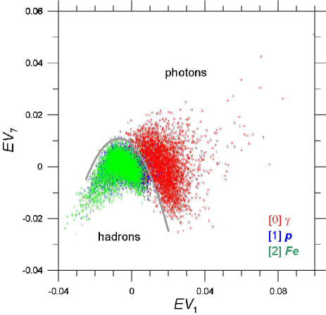
Figure 1: PCA results on the illustrative parameter space. The best separation between nuclei and photons is obtained for the projection on the plane defined by the first and seventh eigenvectors. The thick line misclassifies $4$% of the nuclei as photons and $3$% of the photons as nuclei.

Once the photons have been separated, the same process could be applied, in principle, to the further separation of nuclei among themselves. However, this is a much more complicated problem as can be seen in Fig. 1 or even in Fig. 2, which show that proton and iron nuclei are truly mixed in these parameter space regardless of what projection is chosen for the analysis. The necessity of a more powerful technique is obvious and, as we will show in the following section, a potentially useful diagnostic tool can be obtained by resorting to neural network simulations.

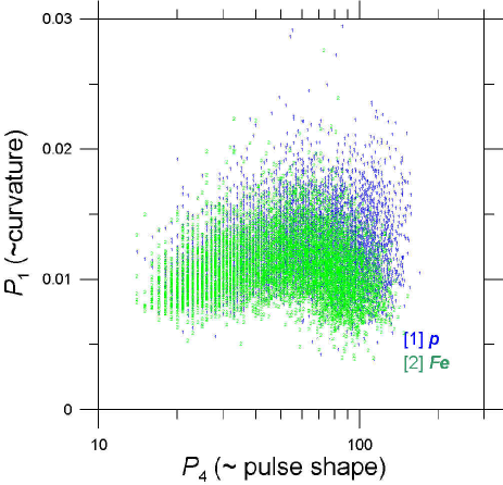
Figure 2: Projection onto the $P_{1}$–$P_{4}$ plane of the sample points, once the photon events have been extracted, showing the difficulty involved in the separation of light and heavy nuclei.

4 Neural Networks applied to nuclei separation

An alternative approach for hadronic primary separation can be obtained by applying neural network technics to the problem.

4.1 Neural Network design

A neural network (NN), is structured in parallel layers of neurons, connected to neurons in adjacent layers. Each connection has a statistic weight (or just weight) since two neurons of the same layer, should not “see” the same input coming from a neuron of the previous layer.

In general terms, a NN is formed by: the input layer, which is connected to the input data vector; an indefinite number of hidden layers and the output layer, the last layer of neurons (see Fig. 3).

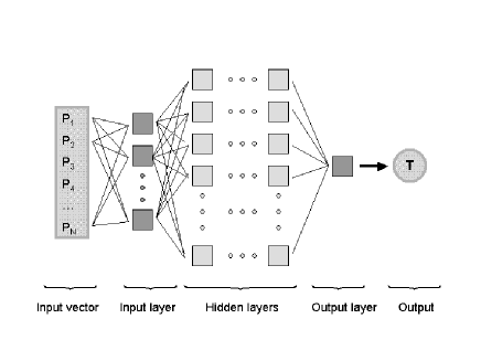
Figure 3: A general network, with an input layer, an hidden layer (multi-layer) and an output layer. Each square box represents a neuron unit showed in Fig. 4.

The elementary processing unit in a NN is the artificial neuron. The information arrives to the neuron from many input channels. The information coming from each channel is linearly transformed by applying a multiplicative weight and an additive bias and fed to a transfer function which gives the neuron output signal (see Fig. 4). The bias parameter b regulates the threshold activation of the neuron (for boolean neurons). But in our case, the bias is one more parameter to be adjusted by the training algorithm.

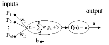
Figure 4: A single neuron from Fig. 3: the input vector p, the weights $w_{i}$ $(i=1,...,R)$, the bias b, the transfer function f and the output signal a. The weight $w_{i}$ shows which importance each input signal has for the neuron.

The training algorithms that we tested, required neurons with differentiable transfer functions. After tests with several transfer functions, we selected basically two types: (a) linear:

$$f(n)=n$$ (7)

and (b) hyperbolic tangent sigmoid:

$$f(n)=\left[\frac{e^{n}-e^{-n}}{e^{n}+e^{-n}}\right]$$ (8)

where:

$$n=\sum_{i=1}^{R}w_{i}p_{i}+b$$ (9)

In our case, the last layer of all networks has one neuron with linear transfer function. All other neurons of the network have hyperbolic tangent sigmoid as transfer function.

For simplicity, we adopt hereafter the following notation in order to represent a network. The notation 7i-10-10-10-1o, for example, means: one input data vector of dimension 7; three layers, each one with 10 neurons (all hyperbolic tangent sigmoid), and the output layer with one neuron(linear). This network has 311 free parameters: 280 weights and 31 biases. Networks of very different architectures and sizes were tested, running from approximately 80 to more than 1100 weights.

The adopted solution was a supervised training algorithm. The training data set $\Phi$, is a collection of Q events, $\Phi=\{\{\textbf{p}_{q},y_{q}\}\}_{q=1}^{Q}$ where $\textbf{p}_{q}$ is the input data vector (the measured parameters that characterize the event) and $y_{q}$ is the identity of the event (atomic mass of the primary nucleus). The supervised training minimizes the difference between the desired output $y_{q}$ and the computed output $a_{q}$, adjusting the weights and biases of the NN.

The minimization function is generally the square error function

$$F(\textbf{x})=\sum_{q=1}^{Q}(y_{q}(\textbf{x})-a_{q})^{2}$$ (10)

where x is the vector formed by the weights and biases of the NN.

The basic backpropagation algorithm [16] was developed for networks with multiple layers of neurons. This is a feedforward algorithm, whose main characteristic is that the process of weight adjusting progresses from the last to the first neuron layer. Some of the backpropagation algorithms we tested use equation (10) as their minimizing function.

A frequent problem in network training is the lost of generalization capability. The algorithm attains a good training level (i.e., low values of $F(\textbf{x})$) but it is not capable of reproducing the same good performance when faced to an independent test set. This problem can often be traced to the development of some few large weights during the process of minimization of the error function. These large weights are responsible, in turn, for a very sensitive NN, which can react unpredictably when presented with inputs that depart, even slightly, from the original training set.

An attempt to solve this problem, used in the present work, is the Bayesian Regularization Backpropagation Algorithm (BRBA), described by [17] and detailed in [18, 19]. Its minimization function is a modified version of (10), aimed at improving the network generalization capability:

$$F(x(k)) =\alpha(k)\sum_{q=1}^{Q}(y_{q}-a_{q}(k))^{2}+\beta(k)\sum_{i=1}^{\Omega}x(k)^{2}$$ (11)

$$=\alpha(k)E_{er}(k)+\beta(k)E_{x}(k)$$

where $\Omega$ is the number of weights of the NN, $\alpha$ and $\beta$ are parameters that change at each iteration $k$.

Roughly speaking, the term $E_{er}$ is responsible for the network learning, while $E_{w}$ is correlated with its generalization capability because it keeps checked the value of sum of the square of the weights. By minimizing both terms simultaneously, $E_{er}$ and $E_{w}$, one expects an equilibrium between learning and generalization capability.

In all cases after training our networks with a given training data set, their generalization capability was checked with an equivalent independent control set.

4.2 Two components UHECR flux: p-Fe separation

Given a specific problem, there are no rules to design on optimal NN. Each problem is a case study in itself. Therefore, many different NN architectures were tested. Several backpropagation algorithms, number of layers, number of neurons in each layer, transfer functions, number of iterations and input sets of parameters were tried until acceptable results were attained [20].

The best results were obtained by first transforming the parameter space into its eigenvector space employing PCA techniques (reducing at the same time the dimensionality of the input data). As a first example, in Fig. 5, we show the results for a feedforward network 7i-10-10-10-1o.

The input parameters used, $P_{i}$, based in direct observables and reconstructed magnitudes from the surface array detector:

$$P_{1}=\left(\frac{1}{N_{stat}}\right)\sum_{i=1}^{N_{stat}}(vem)_{i}\left(\frac{r_{0,i}}{1000m}\right)^{3}\$$ (12)

$$P_{2}=\left(\frac{1}{N_{stat}}\right)\sum_{i=1}^{N_{stat}}T_{sp,i}\left(\frac{r_{0,i}}{1000m}\right)^{-2}\,$$ (13)

$$P_{3}=\left(\frac{1}{N_{stat}}\right)\sum_{i=1}^{N_{stat}}T_{10,i},$$ (14)

$$P_{4}=\left(\frac{1}{N_{stat}}\right)\sum_{i=1}^{N_{stat}}T_{50,i},$$ (15)

$$P_{5}=\left(\frac{1}{N_{stat}}\right)\sum_{i=1}^{N_{stat}}T_{90,i},$$ (16)

plus initial energy ($P_{6}=E_{0}$), zenith angle ($P_{7}=\theta$) and number of triggered stations ($P_{8}=N_{stat}$); where, for the station i: $(vem)_{i}$ is the signal measured in vertical equivalent muons, $T_{sp,i}$ is the arrival time of the shower plane, $r_{0,i}$ is the distance to the shower axis and $T_{j,i}$ (j=10, 50, 90) are the rising times, at which j% of the integral value of the signal is attained.

A set of cuts was applied to remove events too far from the average behavior of the parameter distributions. The cuts, described in Table 1, eliminate roughly $1/4$ of the events.

Table 1: The cuts eliminate roughly 1/4 of the events. The remaining 3/4 events were randomly split into training and independent control sets.

Cuts
$40\leq P_{1}\leq 3\times 10^{5}$
$7\times 10^{-3}\leq P_{2}\leq 20$
$3\times 10^{-2}\leq P_{3}\leq 80$
$3\leq$ P${}_{5}\leq 250$
$P_{8}=N_{stat}\geq 4$

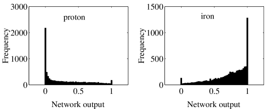
Figure 5: Results of the application of a trained feedforward network to an independent control sample of 13000 events triggered by protons and iron nuclei. The network was trained to output a value of zero (one) for a proton(iron) primary. Tails, therefore, correspond to misclassified events. Only surface array information was included.

The network was trained to output desired $0$ for protons and $1$ for iron nuclei. The training set had 10000 events (5000 for each kind of nucleus).

Fig. 5 shows the result of applying the trained network to independent control samples of 13000 events each one.

If we assume that an output $\leq 0.5$ identifies the event as proton generated and an output$>0.5$ signals to an iron nucleus, then the misclassification probabilities for proton and iron nuclei are, respectively, $P_{p}\sim 27$% and $P_{Fe}\sim 16$%.

In order to asses the impact of using information coming from hybrid events, we performed an additional run including also $X_{max}$. The corresponding output is showed in Fig. 6. A noticeable improvement shows up clearly as the misclassification probability goes down to $\sim 12$% for protons and $\sim 12$% for iron. Furthermore, the number of ambiguous events with intermediate results between 0 and 1 diminishes noticeably producing a cleaner output.

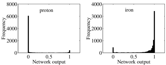
Figure 6: Same as Fig. 5, but now hybrid events were considered (basically through the inclusion of $X_{max}$). A much clearer separation is obtained, despite some events are still misclassified.

Since each shower was reused 20 times to simulate ground events, those events may not be completely independents themselves. This could result in some artificial improvement of the network response. To check this possibility, we eliminated the shower repetitions, lowering the number of available events by a factor of 20, but guaranteing the independence of the events.

We use the same network architecture as before, but this time only one cut was applied, $P_{8}=N_{stat}\geq 4$, since additional cuts would eliminate too many events hindering the analysis. The training set had 900 events (450 of each kind of nucleus) and the independent control samples had roughly 480 events.

The misclassification probabilities for proton and iron nuclei were, respectively, $P_{p}\sim 26$% and $P_{Fe}\sim 20$% for surface events. The same misclassification probabilities, for hybrid events, were $P_{p}\sim 13$% and $P_{Fe}\sim 13$% for proton and iron nuclei. Therefore, there was no artificial improvement in network results because of the not fully independence of the events in the former sample. Note also that this result holds even when the second, completely independent sample, had less cuts in parameter space, which should worsen the results.

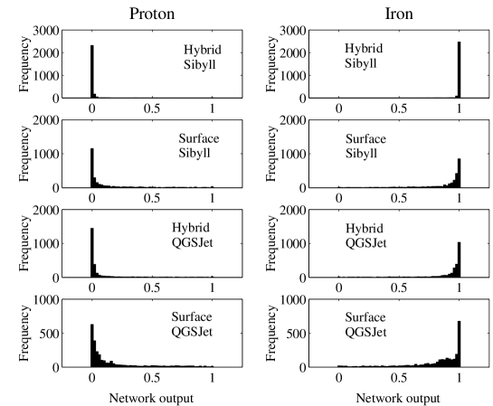
Figure 7: The proton(iron) control samples simulated by the network are in left(right) histograms. The top(down) four histograms were simulated with Sibyll(QGSJet) events. The networks trained with Sibyll events had thinner and clearer output distributions.

In order to maximize the number of events available, training and control data sets of mixed events, of QGSJet and Sibyll interaction models, were used in the previous examples, which hampers the performance of the networks. From now on we show networks simulated with either QGSJet or Sibyll events. Special care was put in selecting equivalent samples of QGSJet and Sibyll events with the same distribution in initial energy $E_{0}$ and zenith angle.

The training set had 6000 events (3000 of each nucleus) and the control independent samples had 2500 events of each nuclei. The same network architecture 7i-10-10-10-1o and the same procedures used before were applied. The results of simulating QGSJet and Sibyll events separately are shown in Fig. 7.

The four upper histograms are the outputs of networks simulated with Sibyll control samples while the four lower histograms correspond to networks simulated with QGSJet control samples. Results are presented for surface and hybrid events. The networks simulated with Sibyll events shows thinner pics around the desired outputs (0 for proton and 1 for iron) and their distributions have a smaller number of ambiguous events than in the case of QGSJet.

The misclassification probabilities of proton and iron nuclei, with surface and hybrid events are in Table 2.

Table 2: The misclassification probabilities of proton($P_{p}$) and iron ($P_{Fe}$) nuclei for networks simulated with control independent samples of different hadronic models.

Hadronic model	Detection	$P_{p}$(%)	$P_{Fe}$(%)
Sibyll	Hybrid	1	1
Sibyll	Surface	12	10
QGSJet	Hybrid	8	9
QGSJet	Surface	15	14

As expected, the results for the misclassification probabilities are much better than in the previous examples, where mixed hadronic interaction models were used.

Table 2 shows that the improvement in misclassification probabilities when going from surface to hybrid events is, for Sibyll events, one order of magnitude. For QGSJet the improving is roughly a factor of two.

In the case of pure surface events, QGSJet and Sibyll misclassification probabilities are approximately equivalent, with a slight advantage in favor of Sibyll. Nevertheless, in the case of hybrid events, those probabilities are very different, being a factor of 10 smaller for Sibyll than for QGSJet. The QGSJet hadronic model has a higher multiplicity than Sibyll, which produces a larger $X_{max}$ dispersion ($\sigma_{X_{max}}^{2}$) and more fluctuations [21]. Apparently, the networks had more difficult in training and recognition of these noisier data sets.

In order to study the effect of our lack of knowledge about the true hadronic interaction model operating in nature at these energies, we trained networks with events simulated with one hadronic model and tested them afterwards with events simulated with the other hadronic interaction model. The same network architecture was used as before. The corresponding misclassification probabilities of control samples are shown in Table 3.

Table 3: The same as in Table 2, but different hadronic interaction models were used for training and testing.

Hadronic model
Trained	Tested	Detection	Pp(%)	PFe(%)
Sibyll	QGSJet	Hybrid	18	15
Sibyll	QGSJet	Surface	27	21
QGSJet	Sibyll	Hybrid	6	10
QGSJet	Sibyll	Surface	21	17

Table 3 shows the important result, that NN should be able to classify primary identity correctly, at least in 70 % of the events, independently of the hadronic interaction model used in the simulations.

Furthermore, if the true hadronic interaction model is unknown, the safest bet is to train with QGSJet and, when possible, to limit the analysis to hybrid events.

The tests performed on binary mixture of proton and iron nuclei show that NN are capable of acceptable classification almost on an event by event bases. However, a binary model for the flux of UHECR, formed only by proton and iron nuclei, is not realistic. If heavy nuclei, say iron, arrive at the top of atmosphere, lighter nuclei should arrive too, even if only due to photodisintegration via interactions with the infrared background in the intergalactic medium. Therefore, we expanded the same NN analysis to a group of eight different nuclei.

4.3 Multi-component UHECR flux: 8 different nuclei

A flat mass spectrum, composed by a mixture of 8 nuclei, was used for training: ¹H, ⁴He, ¹²C, ¹⁶O, ²⁴Mg, ²⁸Si, ⁴⁰Ca and ⁵⁶Fe.

As in the previous case, we tested different NN architectures, learning and training algorithms and sets of parameters. This time, unfortunately, we were unable to design a NN capable of adequately separating individual events.

Consequently, we limited our attempts to a statistical characterization of the mass spectrum.

We were forced to apply additional cuts to the sample of events, based on a series of curve fittings to the lateral distribution of the individual showers. The curve fittings characterize the shape of the lateral distribution function, the curvature of the shower, and the radial dependence of the time structure of the shower front:

$$\it(vem)-(vem)_{90,min}\ =a_{pe}\left(\frac{r}{1000}\right)^{b^{pe}}$$ (17)

$$\it t_{00}\ =a_{0}\left(\frac{r}{1000}\right)^{b^{0}}$$ (18)

$$\it t_{50}-t_{50,min}\ =a_{50}\left(\frac{r}{1000}\right)^{b^{50}}$$ (19)

$$\it t_{90}-t_{90,min}\ =a_{90}\left(\frac{r}{1000}\right)^{b^{90}}$$ (20)

The cuts were applied on the bases of the value of some of the fitted parameters in eq. (17)-(20). The new cuts are given explicitly in Table 4. Again, only high flyers were eliminated. Restrictions were also applyed on the linear regression of the various fittings, $\rho_{i}$. We added an energy cut in energy, similar to Auger energy threshold.

Table 4: The cuts of Table 1 and Table 4, applied together, eliminate roughly 2/3 of the events.

		Cuts
$E_{0}>10^{19}$ eV		$-5\leq b_{pe,i}\leq 0$		$0\leq b_{0,i}\leq 7$
$0\leq b_{50,i}\leq 3$		$0\leq b_{90,i}\leq 2.5$		$\rho_{i}\geq 0.85$

Since event-by-event classification proved too unreliable, we limited ourselves to the statistical determination of the average atomic mass of different composition spectra. As an example we used, arbitrarily, simulated composition spectra of the form $dN/dA\propto A^{\nu}$, with $\nu=-0.5,0.0,0.5,1.0$ and 2.0.

For each value of $\nu$, $1000$ mass spectra of 300 events each, were used to calculate the distribution function of the estimated average mass.

The median output of the network for each nucleus was re-scaled to its actual atomic mass by fitting an exponential function. The criterion used to select among different neural networks was, simultaneously, the goodness of the exponential fitting and the dynamical range of the output between proton and iron.

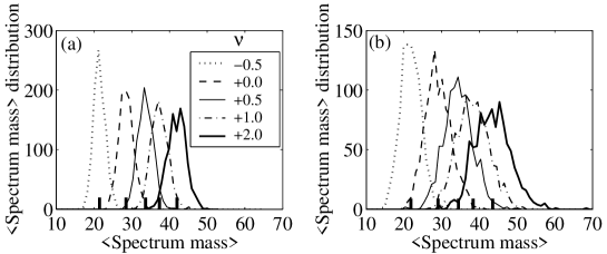
Figure 8: Mass average for 1000 samples of 300 events each simulated with network 7i-4-4-4-1o, for (a) hybrid events (i.e., with $X_{max}$) and (b) pure surface events (i.e., without $X_{max}$). The vertical thick lines are, the true values of the average spectral mass for each $\nu$.

Fig. 8 shows the estimated average masses for different spectral indices $\nu$ for both, hybrid (a) and pure surface events (b). The vertical thick lines are the true values of the average spectral mass for each $\nu$.

We used the set of parameters given by equations (12-16) plus energy, zenith angle and number of triggered stations. The network 7i-4-4-4-1o presented the largest dynamical range between the proton and iron control sample medians among all the network architectures tested. The cuts of Table 1 and Table 4 reduced 2/3 the number of selected events. Therefore, we mixed our QGSJet and the Sibyll samples first to keep a higher number of events for training. This means that the results presented here are a worst case scenario.

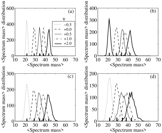
Figure 9: The same of Fig. 8. (a) - Sibyll, hybrid detection; (b) - Sibyll, surface detection; (c) - QGSJet, hybrid detection; (d) - QGSJet, surface detection. Statistical parameters from these distributions are on Table 5.

The errors in the average value of the distributions is of the order of 7% for hybrid (Fig. 8.a) and 12% for surface (Fig. 8.b) events (see Table 5).

Table 5: Statistical parameters of distributions from Fig. 8 and Fig. 9. $\langle A_{t}\rangle$ is the true average distribution (vertical thick lines), $\sqrt{\sigma^{2}}$ is the standard deviation error, $\frac{\sqrt{\sigma^{2}}}{\langle A_{t}\rangle}$ is standart mean error.

			Hybrid detec.		Surface detec.
H. model	$\nu$	$\langle A_{t}\rangle$	$\sqrt{\sigma^{2}}$	$\frac{\sqrt{\sigma^{2}}}{\langle A_{t}\rangle}$ (%)	$\sqrt{\sigma^{2}}$	$\frac{\sqrt{\sigma^{2}}}{\langle A_{t}\rangle}$ (%)
QGSJet	-0.5	21.45	1.59	7	2.79	13
+	+0.0	28.50	1.90	7	3.45	12
Sibyll	+0.5	33.68	2.06	6	3.96	12
	+1.0	37.35	2.28	6	4.29	11
	+2.0	42.00	2.42	6	4.82	11
Sibyll	-0.5	21.45	0.81	4	1.32	6
	+0.0	28.50	0.99	3	1.61	6
	+0.5	33.68	1.14	3	1.84	5
	+1.0	37.35	1.13	3	1.92	5
	+2.0	42.00	1.16	3	2.10	5
QGSJet	-0.5	21.45	1.74	8	2.20	10
	+0.0	28.50	1.99	7	2.64	10
	+0.5	33.68	2.28	7	3.29	10
	+1.0	37.35	2.43	7	3.40	9
	+2.0	42.00	2.55	6	3.61	9

The same analysis, but discriminating by hadronic interaction model is presented in Fig. 9. The training set had 12,000 events (1,500 for each nucleus) and control samples had 2,000 events for each nucleus. The upper panels show the networks trained and simulated with Sibyll events, while the lower panels show the same but for QGSJet events.

As in the case of the proton-iron mixture, the networks were able to classify better when trained with Sibyll events than with QGSJet.

The errors on the determination of the average mass of the distributions are given in Table 5. For Sibyll(QGSJet) events, they were of the order of 6%(10%), for surface detection, and can go down by as much as a factor of two for hybrid events.

With the aim of testing the effect of our lack of knowledge of the true hadronic interaction model, we trained NN with events of one interaction model and simulated them with events of the other interaction model. The tested networks were the same as in the previous example.

The networks trained with Sibyll events and tested with QGSJet events presented smaller standard deviation and standard mean error than those trained with QGSJet and simulated with Sibyll (see, Table 6).

In the worst possible scenario, in which we have only surface information and employ the wrong hadronic interaction model, our neural networks can still calculate the average of the mass spectrum with an error inferior to 20%.

These results show, surprisingly, that NN are only weakly dependent of the hadronic interaction model used.

Table 6: The same of Table 5, but now the networks were trained and tested with events of different hadronic models.

Had. model				Hybrid det.		Surface det.
Trained	Tested	$\nu$	$\langle A_{t}\rangle$	$\sqrt{\sigma^{2}}$	$\frac{\sqrt{\sigma^{2}}}{\langle A_{t}\rangle}$ (%)	$\sqrt{\sigma^{2}}$	$\frac{\sqrt{\sigma^{2}}}{\langle A_{t}\rangle}$ (%)
Sibyll	QGSJet	-0.5	21.45	2.43	11	3.58	17
		+0.0	28.50	2.88	10	3.93	14
		+0.5	33.68	3.02	9	4.21	13
		+1.0	37.35	3.36	9	4.25	11
		+2.0	42.00	3.38	8	4.38	10
QGSJet	Sibyll	-0.5	21.45	3.43	16	4.57	21
		+0.0	28.50	4.98	17	5.18	18
		+0.5	33.68	5.94	18	5.90	18
		+1.0	37.35	6.43	17	6.48	17
		+2.0	42.00	6.91	16	6.72	16

5 Conclusion

In the present work we showed the potential of both PCA and Neural Networks applied to mass composition analysis of UHECRs.

In particular, we studied mass discrimination in three kinds of cosmic ray mixtures: (a) photon-nuclei, (b) proton-iron and (c) a mass spectrum comprising eight nuclei running from proton to iron.

In cases (a) and (b) we showed that event by event classification was possible while, in a multi-component mixture, only a statistical characterization of the mass spectrum is possible.

The PCA method was applied to the problem of separating photons from hadrons. In this way, and for hybrid events, we were able to attain a probability of misidentification of $\sim 3$% for photons $\sim 4$% for hadrons (p and Fe). Nevertheless, we were unable to separate nuclei among themselves by using PCA alone. Neural networks were used to attack this problem.

In the case of binary mixtures of proton and iron, we were able to design neural networks whose misclassification probabilities are 12%(1%) and 10%(1%) for proton and iron with surface(hybrid) detection, for Sibyll training and testing. For QGSJet events, on the other hand, the misclassification probabilities are 15%(8%) and 14%(9%) for proton and iron with surface(hybrid) detection. The QGSJet hadronic model generates noisier shower than Sibyll because of its higher multiplicity. Apparently, the networks had more difficulty in train and testing the noisier QGSJet event sets.

Since the true hadronic interaction model at UHECR energies is still very much under debate, we also trained networks with events of one hadronic model and simulated them with an independent control sample made up of events of the other hadronic model. The tests showed that the networks are able to classify correctly, at least 70% of the events (iron or proton, surface or hybrid detection), independently of the assumptions made on the hadronic interaction model.

For a mixture of eight nuclei, we were unable to design a network capable of discrimination on an event-by-event bases. Therefore, we attempted only the statistical determination of the average atomic mass of different mass spectra. As an example, we show results here for composition spectra of the form $dA/dN\propto A^{\nu}$, with $\nu=-0.5,0.0,0.5,1.0$ and 2.0.

For networks trained with a mixture of QGSJet and Sibyll events, the errors in the average of mass spectrum distributions were of order of 12% (7%) for surface(hybrid) detection. When separating the events by hadronic model, the errors in the determination of the average mass of the spectra went down to $\sim$ 6%(3%) for Sibyll events, and $\sim$ 10%(7%) for QGSJet events, for surface(hybrid) detection.

A weak dependence with hadronic interaction model was confirmed again for the NN, by training and testing the same network with different hadronic interaction models. The errors incurred in the determination of the average spectral mass, in this case, were less than 20%, for surface or hybrid detection regardless of the assumed model.

6 Acknowledgments

This work was supported by the Brazilian agencies CAPES, CNPq and FAPESP. The authors thank Jeferson A. Ortiz and Vitor de Souza for useful discussions.

References

- [1] K. Greisen, Phys. Rev. Lett. 16 (1966) 748; G. T. Zatsenpin, V. A. Kuz’min, Zh. Eksp. Teor. Fiz. Pis’ma Red. 4 (1966) 144 .
- [2] A. M. Hillas, Annu. Rev. Astron. Astrophys. 22 (1984) 425.
- [3] V. S. Berezinsky, M. Kachelriess, A. Vilenkin, Phys. Rev. Lett. 79 (1997) 237.
- [4] Auger Collaboration, Nucl. Inst. and Meth. A 523 (2004) 50 .
- [5] EUSO Collaboration, www.euso-mission.org.
- [6] P. Billoir, Auger technical note GAP-00-025 (2000).
- [7] J. D. Bird et al., Astrophys. J. 441 (1995) 144.
- [8] F. Halzen, A. R. Vazquez, T. Stanev, H. P. Vankov, Astropar. Phys. 3 (1995) 151.
- [9] M. Nagano et al., Astropart. Phys. 13 (2000) 4.
- [10] M. Ave et al., Phys. Rev. Lett. 85 (2000) 2244.
- [11] S. J. Sciutto, in Proceedings of 27th International Cosmic Ray Conference, Hamburg, Germany, 2001 (Copernicus Gesellshaft, Katlemburg-Lindau, 2001) p 237; avaliable electronically, www.fisica.unlp.edu.ar/auger/aires
- [12] N. N. Kalmykov, S. S. Ostapchenko, A. I. Pavlov, Nucl. Phys. (Proc. Suppl.) 52B (1997) 17.
- [13] R. S. Fletcher, T. K. Gaisser, P. Lipari, T. Stanev, Phys. Rev. D 50 (1994) 5710.
- [14] M. H. Hassoun, Fundamentals of Artificial Neural Networks (1995) (The MIT Press, Massachusetts, U.S.).
- [15] G. A. Medina-Tanco, S. J. Sciutto, in Proceedings of 27th ICRC, Hamburg, Germany, 2001 (Copernicus Gesellshaft, Katlemburg-Lindau, 2001) p 518.
- [16] D. E. Rummelhart, J. McCelelland, Parallel Distributed Processing (1986) (The MIT Press, Cambridge, Massachusetts).
- [17] H. Demuth, M. Beale, Neural Network Tool Box -MATLab - Use’s Guide (1999), verson 4.
- [18] F. D. Foresee, and M. T. Hagan, in Proceedings of the 1997 Inter. Joint Conf. on Neural Network (1997) pp 1930-1935.
- [19] M. T. Hagan, H. B. Demuth, M. Beale, Neural Network Design (1996), (PWS Publishing Company, Boston,).
- [20] G. A. Medina-Tanco, S. J. Sciutto, A. K. O. Tiba, in Proceedings of 28th International Cosmic Ray Conference, Tsukuba, Japan, (2003).
- [21] J. Alvarez-Muñiz et al., Phys. Rev. D 69 (2004) 103003.