Third-order perturbative solutions in the Lagrangian perturbation theory with pressure

Abstract

Lagrangian perturbation theory for cosmological fluid describes structure formation in the quasi-nonlinear stage well. We present a third-order perturbative equation for Lagrangian perturbation with pressure in both the longitudinal and transverse modes. Then we derive the perturbative solution for simplest case.

I Introduction

The structure formation scenario based on gravitational instability has been studied for a long time. The Lagrangian perturbative method for the cosmological fluid describes the nonlinear evolution of density fluctuation rather well. Zel’dovich zel proposed a linear Lagrangian approximation for dust fluid. This approximation is called the Zel’dovich approximation (ZA) zel ; Arnold82 ; Shandarin89 ; buchert89 ; coles ; saco . ZA describes the evolution of density fluctuation better than the Eulerian approximation Munshi94 ; Sahni96 ; yoshisato . After that, the second- and the third-order perturbative solution for dust fluid were derived Barrow93 ; Bouchet92 ; Bouchet95 ; Buchert92 ; Buchert93 ; Buchert94 ; Catelan95 ; Sasaki98 .

Recently the effect of the pressure in the cosmological fluid has been considered. At first, the effect of the pressure is originated from velocity dispersion using the collisionless Boltzmann equation BT ; budo . Buchert and Domínguez budo showed that when the velocity dispersion is regarded as small and isotropic it produces effective ”pressure” or viscosity terms. Furthermore, they posited the relation between mass density $\rho$ and pressure $P$, i.e., an ”equation of state”. Adler and Buchert Adler99 have formulated the Lagrangian perturbation theory for a barotropic fluid. Morita and Tatekawa Morita01 and Tatekawa et al. Tatekawa02 solved the Lagrangian perturbation equations for a polytropic fluid up to the second order. Hereafter, we call this model the ”pressure model”.

Although the higher-order perturbative solution is expected to improve the approximation, there is a counterargument. Let us consider the evolution of the spherical void for dust fluid. Because the exact solution has already been derived, we can discuss the accuracy of the perturbative solutions. In this case, when we increase the order of Lagrangian approximation, contrary to expectation, the description becomes worse Munshi94 ; Sahni96 ; Tatekawa05 . Especially, when we stop the order of the perturbation until even order (the second-order), the perturbative solution describes the contraction of a void at a later.

For the pressure model, although we do not know the exact solution for the evolution of the spherical void, the same problem may arise. In fact, according to a comparison between the first-order solution and the full-order numerical solution for the spherical symmetric model, the difference of these solutions obviously appears at a late time (density fluctuation $\delta>1$ or $\delta<-0.5$)  Tatekawa04B .

In this paper, we present the third-order perturbative equation for the pressure model. Then we derive the perturbative solution for the simplest case, i.e., where the background is given by the Einstein-de Sitter (E-dS) Universe model and the polytropic index $\gamma=4/3$. Furthermore, we compare the evolution of the density fluctuation between the first-, second-, and third-order approximations for one-dimensional model.

This paper is organized as follows. In Sec. II, we present a Lagrangian description of basic equations for cosmological fluids. In Sec. III, we show perturbative equations and derive perturbative solutions for the pressure model up to the third order. In Sec. III.1, we show the perturbative equations and solutions of the first- and the second-order perturbation. For the higher-order perturbation, we ignore the first-order transverse modes. In Sec. III.2, we present the perturbative equations for the third-order approximation. In general, it is extremely hard to solve the third-order perturbative equations. Therefore in Sec. III.3, we derive the solutions for the simplest case (E-dS Universe model, $\gamma=4/3$).

In Sec. IV, we introduce spacial symmetry. We consider a planar model and compare the evolution of the density fluctuation between the first-, second-, and third-order approximations. In Sec. V, we summarize our conclusions.

In Appendix A, we present the second-order perturbative equation for a spherical symmetric model in the pressure model. Because of mode-coupling of the first-order perturbations, it seems difficult to solve.

II Basic equations

Here we briefly introduce the Lagrangian description for cosmological fluid. In the comoving coordinates, the basic equations for cosmological fluid are described as

$$\frac{\partial\delta}{\partial t}+\frac{1}{a}\nabla_{x}\cdot\{\bm{v}(1+\delta)\} = 0\,,$$ (1)

$$\frac{\partial\bm{v}}{\partial t}+\frac{1}{a}(\bm{v}\cdot\nabla_{x})\bm{v}+\frac{\dot{a}}{a}\bm{v} = \frac{1}{a}\tilde{\bm{g}}-\frac{1}{a\rho}\nabla_{x}P\,,$$ (2)

$$\nabla_{x}\times\tilde{\bm{g}} = \bm{0}\,,$$ (3)

$$\nabla_{x}\cdot\tilde{\bm{g}} = -4\pi G\rho_{b}a\delta\,,$$ (4)

$$\delta \equiv \frac{\rho-\rho_{b}}{\rho_{b}}\,.$$ (5)

In the Eulerian perturbation theory, the density fluctuation $\delta$ is regarded as a perturbative quantity. On the other hand, in the Lagrangian perturbation theory, the displacement from homogeneous distribution is considered.

$$\bm{x}=\bm{q}+\bm{s}(\bm{q},t)\,,$$ (6)

where $\bm{x}$ and $\bm{q}$ are the comoving Eulerian coordinates and the Lagrangian coordinates, respectively. $\bm{s}$ is the displacement vector that is regarded as a perturbative quantity. From Eq. (6), we can solve the continuous equation Eq. (1) exactly. Then the density fluctuation is given in the formally exact form.

$$\delta=1-J^{-1},~{}~{}J\equiv\det\left(\frac{\partial x_{i}}{\partial q_{j}}\right)\,.$$ (7)

$J$ means the Jacobian of the coordinate transformation from Eulerian $\bm{x}$ to Lagrangian $\bm{q}$. Therefore, when we derive the solutions for $\bm{s}$, we can know the evolution of the density fluctuation.

The peculiar velocity is given by

$$\bm{v}=a\dot{\bm{s}}\,.$$ (8)

Then we introduce the Lagrangian time derivative:

$$\frac{\rm d}{{\rm d}t}\equiv\frac{\partial}{\partial t}+\frac{1}{a}\bm{v}\cdot\nabla_{x}\,.$$ (9)

Taking divergence and rotation of Eq. (2), we obtain the evolution equations for the Lagrangian displacement:

$$\nabla_{x}\cdot\left(\ddot{\bm{s}}+2\frac{\dot{a}}{a}\dot{\bm{s}}-\frac{\kappa\gamma\rho_{b}^{\gamma-1}}{a^{2}}J^{-\gamma}\nabla_{x}J\right) = -4\pi G\rho_{b}(J^{-1}-1)\,,$$ (10)

$$\nabla_{x}\times\left(\ddot{\bm{s}}+2\frac{\dot{a}}{a}\dot{\bm{s}}\right) = 0\,,$$ (11)

where $(\dot{})$ means the Lagrangian time derivative (Eq. (9)). To solve the perturbative equations, we decompose the Lagrangian perturbation to the longitudinal and transverse modes:

$$\bm{s} = \nabla S+\bm{s}^{T}\,,$$ (12)

$$\nabla\cdot\bm{s}^{T} = 0\,,$$ (13)

where $\nabla$ means the Lagrangian spacial derivative.

Here we expand the Jacobian:

$$J = 1+s_{i,i}+\frac{1}{2}\left(s_{i,i}s_{j,j}-s_{i,j}s_{j,i}\right)+\det\left(s_{i,j}\right)$$ (15)

$$= 1+\nabla^{2}S+\frac{1}{2}\left\{(\nabla^{2}S)^{2}-S_{,ij}S_{,ji}-s^{T}_{i,j}s^{T}_{j,i}-2S_{,ij}s^{T}_{j,i}\right\}$$

$$+\det\left(S_{,ij}+s^{T}_{i,j}\right)\,.$$

Because Eqs. (10) and (11) include the Eulerian spacial derivative, we change to the Lagrangian spacial derivative.

$$\frac{\partial}{\partial x_{i}} = \frac{\partial}{\partial q_{i}}-s_{j,i}\frac{\partial}{\partial x_{j}}$$

$$= \frac{\partial}{\partial q_{i}}-s_{j,i}\frac{\partial}{\partial q_{j}}+s_{j,i}s_{k,j}\frac{\partial}{\partial x_{k}}$$

$$= \frac{\partial}{\partial q_{i}}-s_{j,i}\frac{\partial}{\partial q_{j}}+s_{j,i}s_{k,j}\frac{\partial}{\partial q_{k}}+\cdots\,.$$

III The Lagrangian perturbative solutions

III.1 The first- and second-order perturbative solutions

From Eqs. (10) and (11), we obtain the first-order perturbative equations:

$$\nabla^{2}\left(\ddot{S}^{(1)}+2\frac{\dot{a}}{a}\dot{S}^{(1)}-4\pi G\rho_{b}S^{(1)}-\frac{\kappa\gamma\rho_{b}^{\gamma-1}}{a^{2}}\nabla^{2}S^{(1)}\right) = 0\,,$$ (16)

$$\nabla\times\left(\ddot{\bm{s}}^{T(1)}+2\frac{\dot{a}}{a}\dot{\bm{s}}^{T(1)}\right) = {\bm{0}}\,.$$ (17)

The first-order solutions for the longitudinal mode depend on spacial scale. Therefore the solutions are described with a Lagrangian wavenumber. In this paper, we discuss only perturbative solutions in the E-dS Universe model.

$$\widehat{S}^{(1)}(\bm{K},t) = C^{+}(\bm{K})D^{+}(\bm{K},t)+C^{-}(\bm{K})D^{-}(\bm{K},t)\,,$$ (18)

$$D^{\pm}(\bm{K},t) = \left\{\begin{array}[]{lcl}t^{-1/6}{\cal J}_{\pm\nu}(A|\bm{K}|t^{-\gamma+4/3})&\mbox{for}&\gamma\neq\frac{4}{3}\,,\\ t^{-1/6\pm\sqrt{25/36-B|\bm{K}|^{2}}}&\mbox{for}&\gamma=\frac{4}{3}\,,\\ \end{array}\right.$$ (21)

$$A\equiv\frac{3\sqrt{\kappa\gamma}(6\pi G)^{(1-\gamma)/2}}{|4-3\gamma|},~{}B\equiv\frac{4}{3}\kappa(6\pi G)^{-1/3}\,,$$

where ${\cal J}$ means Bessel function. $C^{\pm}(\bm{K})$ is given by the initial condition.

For the transverse mode, the solutions are same as for dust model:

$${\bf s}^{T(1)}\propto\mbox{const.},t^{-1/3}\,.$$ (22)

The transverse mode does not have a growing solution. Therefore, in first-order approximation, the longitudinal mode dominate during evolution. Hereafter we consider only the longitudinal mode solutions for the first-order solutions.

From Eqs. (10) and (11), we obtain the second-order perturbative equations. For the longitudinal mode, the equation becomes

$$\nabla^{2}\left(\ddot{S}^{(2)}+2\frac{\dot{a}}{a}\dot{S}^{(2)}-4\pi G\rho_{b}S^{(2)}-\frac{\kappa\gamma\rho_{b}^{\gamma-1}}{a^{2}}\nabla^{2}S^{(2)}\right)=Q^{L(2)}\,,$$ (23)

$$Q^{L(2)} = 2\pi G\rho_{b}\left[S^{(1)}_{,ij}S^{(1)}_{,ij}-\left(\nabla^{2}S^{(1)}\right)^{2}\right]-\frac{\kappa\gamma^{2}\rho_{b}^{\gamma-1}}{a^{2}}\left(\nabla^{2}S^{(1)}_{,i}\nabla^{2}S^{(1)}_{,i}\right)$$ (24)

$$-\frac{\kappa\gamma(\gamma-1)\rho_{b}^{\gamma-1}}{a^{2}}\left(\nabla^{2}\nabla^{2}S^{(1)}\nabla^{2}S^{(1)}\right)-\frac{\kappa\gamma\rho_{b}^{\gamma-1}}{a^{2}}\left(S^{(1)}_{,ijk}S^{(1)}_{,ijk}+2S^{(1)}_{,ij}\nabla^{2}S^{(1)}_{,ij}\right)\,.$$

For the transverse mode, after some arrangement, we can describe as follows:

$$\nabla^{2}\left(\ddot{s}^{T(2)}_{,i}+2\frac{\dot{a}}{a}\dot{s}^{T(2)}_{,i}\right)=Q_{i}^{T(2)}\,,$$ (25)

$$Q_{i}^{T(2)}=\frac{\kappa\gamma\rho_{b}^{\gamma-1}}{a^{2}}\left(S^{(1)}_{,ijk}\nabla^{2}S^{(1)}_{,jk}+S^{(1)}_{,ij}\nabla^{2}\nabla^{2}S^{(1)}_{,j}-\nabla^{2}S^{(1)}_{,j}\nabla^{2}S^{(1)}_{,ij}-S^{(1)}_{,jk}\nabla^{2}S^{(1)}_{,ijk}\right)\,.$$ (26)

Here we notice for the second-order transverse mode solutions. In the pressure model, even if we consider only the longitudinal mode for the first-order, the second-order perturbation for the transverse mode appears. In dust model, it does not appear. Therefore, when we derive the third-order perturbative solutions, we must consider the second-order transverse mode.

The second-order solutions are formally written as follows:

$$\widehat{S}^{(2)} = -\frac{1}{|\bm{K}|^{2}}\int^{t}{\rm d}t^{\prime}G(\bm{K},t,t^{\prime})\widehat{Q}^{L(2)}(\bm{K},t)\,,$$ (27)

$$\widehat{s}^{T(2)} = -\frac{1}{|\bm{K}|^{2}}\int^{t}{\rm d}t^{\prime}G^{T}(t,t^{\prime})\widehat{Q}^{T(2)}(\bm{K},t)\,,$$ (28)

$$G^{T}(t,t^{\prime}) = 3(t^{\prime}-t^{-1/3}t^{\prime 4/3})\,.$$ (29)

$G^{L}(\bm{K},t,t^{\prime})$ depends on the equation of state. If $\gamma\neq 4/3$ and $\nu=5/(8-6\gamma)$ is not an integer, we have

$$G^{L}(\bm{K},t,t^{\prime}) = -\frac{\pi}{2\sin\nu\pi}\left(-\gamma+\frac{4}{3}\right)^{-1}t^{-1/6}t^{\prime 7/6}\left[\mathcal{J}_{-\nu}\left(A|\bm{K}|t^{-\gamma+4/3}\right)\mathcal{J}_{\nu}\left(A|\bm{K}|t^{\prime-\gamma+4/3}\right)\right.$$ (30)

$$~{}~{}\left.-\mathcal{J}_{\nu}\left(A|\bm{K}|t^{-\gamma+4/3}\right)\mathcal{J}_{-\nu}\left(A|\bm{K}|t^{\prime-\gamma+4/3}\right)\right]\,,$$

and if $\gamma=4/3$,

$$G^{L}(\bm{K},t,t^{\prime}) = -\frac{1}{2b(\bm{K})}t^{-1/6}t^{\prime 7/6}\left(t^{-b(\bm{K})}t^{\prime b(\bm{K})}-t^{b(\bm{K})}t^{\prime-b(\bm{K})}\right)\,,$$ (31)

$$b(\bm{K}) \equiv \sqrt{\frac{25}{36}-B|\bm{K}|^{2}}\,.$$ (32)

The second-order perturbative solution for the case of $\gamma=4/3$ in the E-dS universe model is described by

$$\hat{S}^{(2)}(\bm{K}) = \int{\rm d}\bm{K}^{\prime}~{}\Xi^{L}(\bm{K},\bm{K}^{\prime})E^{L}(\bm{K},\bm{K}^{\prime},t)\,,$$ (33)

$$\hat{s}_{j}^{T(2)}(\bm{K}) = \int{\rm d}{\bf K}^{\prime}~{}\Xi^{T}_{j}(\bm{K},\bm{K}^{\prime})E^{T}(\bm{K},\bm{K}^{\prime},t)\,,$$ (34)

$$\Xi^{L}(\bm{K},\bm{K}^{\prime}) = -\frac{1}{(2\pi)^{3}}\frac{1}{|\bm{K}|^{2}}\left[\frac{1}{3}\left\{(\bm{K}^{\prime}\cdot(\bm{K}-\bm{K}^{\prime}))^{2}-|\bm{K}^{\prime}|^{2}|\bm{K}-\bm{K}^{\prime}|^{2}\right\}\right.$$ (35)

$$~{}~{}\left.+B\left\{\frac{4}{3}|\bm{K}^{\prime}|^{2}|\bm{K}-\bm{K}^{\prime}|^{2}(\bm{K}^{\prime}\cdot(\bm{K}-\bm{K}^{\prime}))+\frac{1}{3}|\bm{K}^{\prime}|^{4}|\bm{K}-\bm{K}^{\prime}|^{2}\right.\right.$$

$$~{}~{}~{}~{}~{}~{}~{}~{}~{}~{}~{}~{}\left.\left.+\left((\bm{K}^{\prime}\cdot(\bm{K}-\bm{K}^{\prime}))^{3}+2|\bm{K}-\bm{K}^{\prime}|^{2}(\bm{K}^{\prime}\cdot(\bm{K}-\bm{K}^{\prime}))^{2}\right)\right\}\right]\,.$$

$$\Xi^{T}_{j}(\bm{K},\bm{K}^{\prime}) = -\frac{i}{(2\pi)^{3}}\frac{B}{|\bm{K}|^{2}}|\bm{K}-\bm{K}^{\prime}|^{2}(\bm{K}^{\prime}\cdot(\bm{K}-\bm{K}^{\prime}))$$ (36)

$$~{}~{}~{}~{}\left[(\bm{K}^{\prime}\cdot(\bm{K}-\bm{K}^{\prime}))K^{\prime}_{j}+|\bm{K}-\bm{K}^{\prime}|^{2}K^{\prime}_{j}-|\bm{K}^{\prime}|^{2}(K_{j}-K^{\prime}_{j})-(\bm{K}^{\prime}\cdot(\bm{K}-\bm{K}^{\prime}))(K_{j}-K^{\prime}_{j})\right]\,,$$

$$E^{L}(\bm{K},\bm{K}^{\prime},t) = \frac{1}{2b(\bm{K})}\sum_{(\oplus=\pm)}\sum_{(\otimes=\pm)}\left[\frac{C^{\oplus}(\bm{K}^{\prime})C^{\otimes}(\bm{K}-\bm{K}^{\prime})t^{-1/3\oplus b(\bm{K}^{\prime})\otimes b(\bm{K}-\bm{K}^{\prime})}}{((\oplus b(\bm{K}^{\prime})\otimes b(\bm{K}-\bm{K}^{\prime})-\frac{1}{6})^{2}-b(\bm{K})^{2})}\right]\,,$$ (37)

$$E^{T}(\bm{K},\bm{K}^{\prime},t) = 3\sum_{(\oplus=\pm)}\sum_{(\otimes=\pm)}\left[\frac{C^{\oplus}(\bm{K}^{\prime})C^{\otimes}(\bm{K}-\bm{K}^{\prime})t^{-1/3\oplus b(\bm{K}^{\prime})\otimes b(\bm{K}-\bm{K}^{\prime})}}{(\oplus b(\bm{K}^{\prime})\otimes b(\bm{K}-\bm{K}^{\prime})-\frac{1}{3})(\oplus b(\bm{K}^{\prime})\otimes b(\bm{K}-\bm{K}^{\prime}))}\right]\,,$$ (38)

where $\sum_{(\oplus=\pm)}$ means

$$\sum_{(\oplus=\pm)}(\alpha^{\oplus}\oplus\beta)\equiv(\alpha^{+}+\beta)+(\alpha^{-}-\beta)\,.$$ (39)

III.2 The third-order perturbative equations

The third-order perturbative equation becomes very complicated. Here we introduce scalar quantities generated by Lagrangian perturbation.

$$\mu_{1}({\bm{A}}) \equiv \nabla\cdot{\bm{A}}\,,$$ (40)

$$\mu_{2}({\bm{A}},{\bm{B}}) \equiv \frac{1}{2}\left((\nabla\cdot{\bm{A}})(\nabla\cdot{\bm{B}})-A_{i,j}B_{j,i}\right)\,,$$ (41)

$$\mu_{2}({\bm{A}}) \equiv \mu_{2}({\bm{A}},{\bm{A}})\,,$$ (42)

$$\mu_{3}({\bm{A}}) \equiv \mbox{det}\left(A_{i,j}\right)\,,$$ (43)

where ${\bm{A}}$ and ${\bm{B}}$ are vector quantities.

First, we show the longitudinal mode equation. As in the second-order perturbative equation, we separate the terms of the third-order perturbation from the others. Then the terms consisting of the first- and the second-order perturbations are collected to the source term $Q^{L(3)}$.

$$\nabla^{2}\left(\ddot{S}^{(3)}+2\frac{\dot{a}}{a}\dot{S}^{(3)}-4\pi G\rho_{b}S^{(3)}-\frac{\kappa\gamma\rho_{b}^{\gamma-1}}{a^{2}}\nabla^{2}S^{(3)}\right)=Q^{L(3)}\,.$$ (44)

We consider the source term. Using Eqs. (40)-(43), the terms are written as follows:

$$Q^{L(3)} = 4\pi G\rho_{b}\left[\mu_{1}(S^{(1)}_{,i})^{3}+\mu_{2}(S^{(1)}_{,i},S^{(2)}_{,i}+s^{T(2)}_{i})+\mu_{3}(S^{(1)}_{,i})\right]$$ (45)

$$+\frac{\kappa\gamma\rho_{b}^{\gamma-1}}{a^{2}}\left[\mu_{2}(S^{(1)}_{,i},S^{(2)}_{,i}+s^{T(2)}_{i})+\mu_{3}(S^{(1)}_{,i})\right.$$

$$~{}~{}~{}~{}~{}~{}~{}~{}~{}~{}\left.-S^{(1)}_{,jk}\left\{\partial_{j}\partial_{k}\left(\mu_{1}(S^{(2)}_{,i})+\mu_{2}(S^{(1)}_{,i})\right)\right\}\right.$$

$$~{}~{}~{}~{}~{}~{}~{}~{}~{}~{}\left.+\gamma\partial_{j}\left\{\mu_{1}(S^{(1)}_{,i})~{}\partial_{j}\left(\mu_{1}(S^{(2)}_{,i})+\mu_{2}(S^{(1)}_{,i})\right)\right\}\right.$$

$$~{}~{}~{}~{}~{}~{}~{}~{}~{}~{}\left.+\partial_{j}\left\{S^{(1)}_{,jk}~{}\partial_{k}\left(\mu_{1}(S^{(2)}_{,i})+\mu_{2}(S^{(1)}_{,i})\right)\right\}\right.$$

$$~{}~{}~{}~{}~{}~{}~{}~{}~{}~{}\left.-\left\{(S^{(2)}_{,jk}+s^{T(2)}_{j,k})~{}\partial_{j}\partial_{k}\mu_{1}(S^{(1)}_{,i})-S^{(1)}_{,jk}S^{(1)}_{,kl}~{}\partial_{j}\partial_{l}\mu_{1}(S^{(1)}_{,i})\right\}\right.$$

$$~{}~{}~{}~{}~{}~{}~{}~{}~{}~{}\left.+\partial_{j}\left\{\left(-\gamma\mu_{1}(S^{(2)}_{,i})-\gamma\mu_{2}(S^{(1)}_{,i})+\frac{\gamma(\gamma+1)}{2}\mu_{1}(S^{(1)}_{,i})^{2}\right)\partial_{j}\mu_{1}(S^{(1)}_{,i})\right\}\right.$$

$$~{}~{}~{}~{}~{}~{}~{}~{}~{}~{}\left.+\partial_{j}\left\{-(S^{(2)}_{,jk}+s^{T(2)}_{j,k})~{}\partial_{k}\mu_{1}(S^{(1)}_{,i})+S^{(1)}_{,jk}S^{(1)}_{,kl}~{}\partial_{l}\mu_{1}(S^{(1)}_{,i})\right\}\right.$$

$$~{}~{}~{}~{}~{}~{}~{}~{}~{}~{}\left.-S^{(1)}_{,jk}\partial_{k}\left\{-\gamma\mu_{1}(S^{(1)}_{,i})~{}\partial_{j}\mu_{1}(S^{(1)}_{,i})-S^{(1)}_{,jl}~{}\partial_{l}\mu_{1}(S^{(1)}_{,i})\right\}\right.$$

$$~{}~{}~{}~{}~{}~{}~{}~{}~{}~{}\left.+\partial_{j}\left\{\gamma\mu_{1}(S^{(1)}_{,i})~{}S^{(1)}_{,jk}~{}\partial_{k}\mu_{1}(S^{(1)}_{,i})\right\}\right]\,.$$

The transverse mode also seems complicated. However, if we neglect the first-order transverse mode, the evolution equation is described as

$$-\nabla^{2}\left(\ddot{s}^{T(3)}_{i}+2\frac{\dot{a}}{a}\ddot{s}^{T(3)}_{i}\right)=Q_{i}^{T(3)}\,,$$ (46)

$$Q_{i}^{T(3)} = \left\{S_{,ij}^{(1)}\left(\ddot{s}^{(2)}_{k,j}+2\frac{\dot{a}}{a}\dot{s}^{(2)}_{k,j}\right)\right\}_{,k}-\left\{S_{,jk}^{(1)}\left(\ddot{s}^{(2)}_{i,j}+2\frac{\dot{a}}{a}\dot{s}^{(2)}_{i,j}\right)\right\}_{,k}$$ (47)

$$+\left\{s_{i,j}^{(2)}\left(4\pi G\rho_{b}S^{(1)}_{,jk}+\frac{\kappa\gamma\rho_{b}^{\gamma-1}}{a^{2}}\nabla^{2}S^{(1)}_{,jk}\right)\right\}_{,k}-\left\{s_{j,k}^{(2)}\left(4\pi G\rho_{b}S^{(1)}_{,ij}+\frac{\kappa\gamma\rho_{b}^{\gamma-1}}{a^{2}}\nabla^{2}S^{(1)}_{,ij}\right)\right\}_{,k}$$

$$+\frac{\kappa\gamma\rho_{b}^{\gamma-1}}{a^{2}}\left(\nabla^{2}S_{,il}^{(1)}S_{,jk}^{(1)}S_{,jkl}^{(1)}+\nabla^{2}S_{,il}^{(1)}\nabla^{2}S_{,j}^{(1)}S_{,jl}^{(1)}+\nabla^{2}S_{,ikl}^{(1)}S_{,jk}^{(1)}S_{,jl}^{(1)}\right.$$

$$~{}~{}~{}~{}~{}~{}~{}~{}\left.-S_{,ijk}^{(1)}S_{,jl}^{(1)}\nabla^{2}S_{,kl}^{(1)}-S_{,ij}^{(1)}S_{,jkl}^{(1)}\nabla^{2}S_{,kl}^{(1)}-S_{,ij}^{(1)}S_{,jk}^{(1)}\nabla^{2}S_{,k}^{(1)}\right)\,.$$

III.3 The third-order perturbative solutions – the simplest case

As in the first- and the second-order solutions, the third-order solutions are described with the Lagrangian wavenumber. Following the method used in the second-order solutions, the third-order solution is given by this integration:

$$\widehat{S}^{(3)} = -\frac{1}{|\bm{K}|^{2}}\int_{t_{0}}^{t}{\rm d}t^{\prime}G(\bm{K},t,t^{\prime})\widehat{Q}^{L(3)}(\bm{K},t)\,,$$ (48)

$$\widehat{s}^{T(3)} = -\frac{1}{|\bm{K}|^{2}}\int_{t_{0}}^{t}{\rm d}t^{\prime}G^{T}(t,t^{\prime})\widehat{Q}^{T(3)}(\bm{K},t)\,,$$ (49)

Here we show the third-order perturbative solutions for simplest case, the case of $\gamma=4/3$ in the E-dS Universe model. In this case, the contribution of the gravitational terms and the pressure terms become identical:

$$4\pi G\rho_{b},\frac{\kappa\gamma\rho_{b}^{\gamma-1}}{a^{2}}\propto a^{-3}\,.$$ (50)

Here we write these terms as $M/a^{3}(M=\mbox{const.})$. From the terms described by the multiplication of $S^{(1)}$ and $S^{(2)}$ in $Q^{L}$, the time evolution of a part of the third order perturbation is contributed a

$$F_{1}^{L}(\bm{K},\bm{K}^{\prime\prime},t)$$ (51)

$$\equiv \int^{t}{\rm d}t^{\prime}G(\bm{K},t,t^{\prime})~{}\frac{M}{a(t^{\prime})^{3}}\left(\widehat{S}^{(1)}(\bm{K}^{\prime\prime},t^{\prime})\widehat{S}^{(2)}(\bm{K}-\bm{K}^{\prime\prime},t^{\prime})\right)$$

$$= -\frac{BM}{4b(\bm{K})b(\bm{K}-\bm{K}^{\prime\prime})|\bm{K}|^{2}}~{}t^{-1/2}\int{\rm d}\bm{K}^{\prime}\Xi^{L}(\bm{K}-\bm{K}^{\prime\prime},\bm{K}^{\prime}-\bm{K}^{\prime\prime})$$

$$\sum_{(\oplus=\pm)}\sum_{(\otimes=\pm)}\sum_{(\oslash=\pm)}\left[\frac{C^{\oplus}(\bm{K}^{\prime\prime})C^{\otimes}(\bm{K}^{\prime}-\bm{K}^{\prime\prime})C^{\oslash}(\bm{K}-\bm{K}^{\prime})}{((\otimes b_{2}\oslash b_{3}-\frac{1}{6})^{2}-b_{4}^{2})((\oplus b_{1}\otimes b_{2}\oslash b_{3}-\frac{1}{3})^{2}-b_{5}^{2})}t^{\oplus b_{1}\otimes b_{2}\oslash b_{3}}\right]\,.$$

$$b_{1}\equiv b(\bm{K}^{\prime\prime}),~{}b_{2}\equiv b(\bm{K}^{\prime}-\bm{K}^{\prime\prime}),~{}b_{3}\equiv b(\bm{K}-\bm{K}^{\prime}),~{}b_{4}\equiv b(\bm{K}-\bm{K}^{\prime\prime}),~{}b_{5}\equiv b(\bm{K})\,.$$ (52)

On the other hand, from the terms described by the triplet of $S^{(1)}$ in $Q^{L}$, time evolution of a part of the third order perturbation is contributed as:

$$F_{2}^{L}(\bm{K},\bm{K}^{\prime},\bm{K}^{\prime\prime},t)$$ (53)

$$\equiv \int^{t}{\rm d}t^{\prime}G(\bm{K},t,t^{\prime})~{}\frac{M}{a(t^{\prime})^{3}}\left(\widehat{S}^{(1)}(\bm{K}^{\prime\prime},t^{\prime})\widehat{S}^{(1)}(\bm{K}^{\prime}-\bm{K}^{\prime\prime},t^{\prime})\widehat{S}^{(1)}(\bm{K}-\bm{K}^{\prime},t^{\prime})\right)$$

$$= -\frac{M}{2b(\bm{K})|\bm{K}|^{2}}~{}t^{-1/2}\cdot$$

$$\sum_{(\oplus=\pm)}\sum_{(\otimes=\pm)}\sum_{(\oslash=\pm)}\left[\frac{C^{\oplus}(\bm{K}^{\prime\prime})C^{\otimes}(\bm{K}^{\prime}-\bm{K}^{\prime\prime})C^{\oslash}(\bm{K}-\bm{K}^{\prime})}{(\oplus b_{1}\ominus b_{2}\oslash b_{3}-\frac{1}{3})^{2}-b_{5}^{2}}t^{\oplus b_{1}\ominus b_{2}\oslash b_{3}}\right]\,.$$

When we consider the effect of pressure, even if ${\bm{s}}^{T(1)}={\bm{0}}$, ${\bm{s}}^{T(2)}$ appears. Therefore, the contribution from the multiplication of $S^{(1)}$ and ${\bm{s}}^{T(2)}$ also exists. The contribution from the multiplication of $S^{(1)}$ and ${\bm{s}}^{T(2)}$ is given as follows:

$$F_{3~{}j}^{L}(\bm{K},\bm{K}^{\prime\prime},t)$$ (54)

$$\equiv \int^{t}{\rm d}t^{\prime}G(\bm{K},t,t^{\prime})~{}\frac{M}{a(t^{\prime})^{3}}\left(\widehat{S}^{(1)}(\bm{K}^{\prime\prime},t^{\prime})\widehat{s}_{j}^{T(2)}(\bm{K}-\bm{K}^{\prime\prime},t^{\prime})\right)$$

$$= -\frac{3M}{2b(\bm{K})|\bm{K}|^{2}}~{}t^{-1/2}\int{\rm d}\bm{K}^{\prime}~{}\Xi^{T}_{j}(\bm{K}-\bm{K}^{\prime\prime},\bm{K}^{\prime}-\bm{K}^{\prime\prime})$$

$$\sum_{(\oplus=\pm)}\sum_{(\otimes=\pm)}\sum_{(\oslash=\pm)}\left[\frac{C^{\oplus}(\bm{K}^{\prime\prime})C^{\otimes}(\bm{K}^{\prime}-\bm{K}^{\prime\prime})C^{\oslash}(\bm{K}-\bm{K}^{\prime})}{(\otimes b_{2}\oslash b_{3}-\frac{1}{3})(\otimes b_{2}\oslash b_{3})((\oplus b_{1}\otimes b_{2}\oslash b_{3}-\frac{1}{3})^{2}-b_{5}^{2})}t^{\oplus b_{1}\otimes b_{2}\oslash b_{3}}\right]\,.$$

Next, we consider the third-order transverse mode ${\bm{s}}^{T(3)}$. In the transverse mode, we must make the contribution not only from the multiplication of longitudinal modes, but also from the multiplication of $S^{(1)}$ and ${\bm{s}}^{T(2)}$:

$$F_{1}^{T}(\bm{K},\bm{K}^{\prime\prime},t)$$ (55)

$$\equiv \int^{t}{\rm d}t^{\prime}G^{T}(t,t^{\prime})~{}\frac{M}{a(t^{\prime})^{3}}\left(\widehat{S}^{(1)}(\bm{K}^{\prime\prime},t^{\prime})\widehat{S}^{(2)}(\bm{K}-\bm{K}^{\prime\prime},t^{\prime})\right)$$

$$= -\frac{M}{2b(\bm{K}-\bm{K}^{\prime\prime})|\bm{K}|^{2}}~{}t^{-1/2}\int{\rm d}\bm{K}^{\prime}~{}\Xi^{L}(\bm{K}-\bm{K}^{\prime\prime},\bm{K}^{\prime}-\bm{K}^{\prime\prime})$$

$$\sum_{(\oplus=\pm)}\sum_{(\otimes=\pm)}\sum_{(\oslash=\pm)}\left[\frac{C^{\oplus}(\bm{K}^{\prime\prime})C^{\otimes}(\bm{K}-\bm{K}^{\prime})C^{\oslash}(\bm{K}^{\prime}-\bm{K}^{\prime\prime})}{(\oplus b_{1}\otimes b_{2}\oslash b_{3}-\frac{1}{6})(\oplus b_{1}\otimes b_{2}\oslash b_{3}-\frac{1}{2})((\otimes b_{2}\oslash b_{3}-\frac{1}{6})^{2}-b_{4}^{2})}t^{\oplus b_{1}\otimes b_{2}\oslash b_{3}}\right]\,.$$

$$F_{2}^{T}(\bm{K},\bm{K}^{\prime},\bm{K}^{\prime\prime},t)$$ (56)

$$\equiv \int^{t}{\rm d}t^{\prime}G^{T}(t,t^{\prime})~{}\frac{M}{a(t^{\prime})^{3}}\left(\widehat{S}^{(1)}(\bm{K}^{\prime\prime},t^{\prime})\widehat{S}^{(1)}(\bm{K}^{\prime}-\bm{K}^{\prime\prime},t^{\prime})\widehat{S}^{(1)}(\bm{K}-\bm{K}^{\prime},t^{\prime})\right)$$

$$= -\frac{M}{|\bm{K}|^{2}}~{}t^{-1/2}$$

$$~{}\sum_{(\oplus=\pm)}\sum_{(\otimes=\pm)}\sum_{(\oslash=\pm)}\left[\frac{C^{\oplus}(\bm{K}^{\prime\prime})C^{\otimes}(\bm{K}-\bm{K}^{\prime})C^{\oslash}(\bm{K}^{\prime}-\bm{K}^{\prime\prime})}{(\oplus b_{1}\otimes b_{2}\oslash b_{3}-\frac{1}{6})(\oplus b_{1}\otimes b_{2}\oslash b_{3}-\frac{1}{2})}t^{\oplus b_{1}\otimes b_{2}\oslash b_{3}}\right]\,.$$

$$F_{3}^{T}(\bm{K},\bm{K}^{\prime\prime},t)$$ (57)

$$\equiv \int^{t}{\rm d}t^{\prime}G^{T}(t,t^{\prime})~{}\frac{M}{a(t^{\prime})^{3}}\left(\widehat{S}^{(1)}(\bm{K}^{\prime\prime},t^{\prime})\widehat{s}_{j}^{T(2)}(\bm{K}-\bm{K}^{\prime\prime},t^{\prime})\right)$$

$$= -\frac{3M}{|\bm{K}|^{2}}~{}t^{-1/2}\int{\rm d}\bm{K}^{\prime}~{}\Xi^{T}_{j}(\bm{K}-\bm{K}^{\prime\prime},\bm{K}^{\prime}-\bm{K}^{\prime\prime})$$

$$\sum_{(\oplus=\pm)}\sum_{(\otimes=\pm)}\sum_{(\oslash=\pm)}\left[\frac{C^{\oplus}(\bm{K}^{\prime\prime})C^{\otimes}(\bm{K}-\bm{K}^{\prime})C^{\oslash}(\bm{K}^{\prime}-\bm{K}^{\prime\prime})}{(\otimes b_{2}\oslash b_{3}-\frac{1}{3})(\otimes b_{2}\oslash b_{3})(\otimes b_{1}\oplus b_{2}\oslash b_{3}-\frac{1}{6})(\otimes b_{1}\oplus b_{2}\oslash b_{3}-\frac{1}{2})}t^{\oplus b_{1}\otimes b_{2}\oslash b_{3}}\right]\,.$$

The third-order perturbative solutions for the case of $\gamma=4/3$ in the E-dS Universe model is described with Eqs. (51)-(56). Even if we restrict ourselves to the simplest case, the third-order perturbative solutions become very complicated. For other case, although we can derive the solutions following similar procedures, the solutions may become difficult to analyze structure formation.

IV The time evolution in the planar models

In the previous section, we derived the third-order perturbative solutions for the simplest case. Although we restricted ourselves to the simplest case, the solutions are still complicated. For analyses of the perturbative solutions, we introduce spacial symmetry. If we consider a planar model, the nonlinear terms in the gravitational term disappear. The evolution equation for Lagrangian displacement becomes

$$\ddot{\vec{s}}+2\frac{\dot{a}}{a}\dot{\vec{s}}-4\pi G\rho_{b}\vec{s}=\frac{\kappa\gamma\rho_{b}^{\gamma-1}}{a^{2}(1+\vec{s}_{,1})^{\gamma+1}}\vec{s}_{,11}\,,$$ (58)

where $\vec{s}$ is Lagrangian displacement, not longitudinal mode potential Adler99 . From the expansion of Eq. (58), we obtain perturbative equations.

$$\ddot{\vec{s}}^{(1)}+2\frac{\dot{a}}{a}\dot{\vec{s}}^{(1)}-4\pi G\rho_{b}\vec{s}^{(1)}-\frac{\kappa\gamma\rho_{b}^{\gamma-1}}{a^{2}}\vec{s}^{(1)}_{,11} = 0\,,$$ (59)

$$\ddot{\vec{s}}^{(2)}+2\frac{\dot{a}}{a}\dot{\vec{s}}^{(2)}-4\pi G\rho_{b}\vec{s}^{(2)}-\frac{\kappa\gamma\rho_{b}^{\gamma-1}}{a^{2}}\vec{s}^{(2)}_{,11} = -\frac{\kappa\gamma\rho_{b}^{\gamma-1}}{a^{2}}(\gamma+1)\vec{s}^{(1)}_{,1}\vec{s}^{(1)}_{,11}\,,$$ (60)

$$\ddot{\vec{s}}^{(3)}+2\frac{\dot{a}}{a}\dot{\vec{s}}^{(3)}-4\pi G\rho_{b}\vec{s}^{(3)}-\frac{\kappa\gamma\rho_{b}^{\gamma-1}}{a^{2}}\vec{s}^{(3)}_{,11} = \frac{\kappa\gamma\rho_{b}^{\gamma-1}}{a^{2}}\left[(\gamma+1)(\vec{s}^{(1)}_{,1}\vec{s}^{(2)}_{,11}+\vec{s}^{(2)}_{,1}\vec{s}^{(1)}_{,11})\right.$$ (61)

$$~{}~{}~{}~{}~{}~{}~{}~{}\left.+\frac{(\gamma+1)(\gamma+2)}{2}\left\{(\vec{s}^{(1)}_{,1})^{2}\vec{s}^{(1)}_{,11}\right\}\right]\,.$$

For the simplest case, i.e. the Einstein-de Sitter model and $\gamma=4/3$, using Eqs. (51) and (53), we can describe the perturbative solution for a planar model:

$$\widehat{\vec{s}}^{(1)}(K,t) = C^{+}(K)t^{-1/6+b(K)}+C^{-}(K)t^{-1/6-b(K)}\,,$$ (62)

$$\widehat{\vec{s}}^{(2)}(K,t) = \frac{28i}{9}\int{\rm d}K^{\prime}~{}(K^{\prime}(K-K^{\prime})^{2})E^{L}(K,K^{\prime},t)\,,$$ (63)

$$\widehat{\vec{s}}^{(3)}(K,t) = \frac{784}{81}\int{\rm d}K^{\prime}\int{\rm d}K^{\prime\prime}\left[(K\cdot K^{\prime\prime}\cdot(K-K^{\prime\prime}))(K^{\prime\prime}-K^{\prime})K^{\prime}\right]$$ (64)

$$~{}~{}~{}\sum_{(\oplus=\pm)}\sum_{(\otimes=\pm)}\sum_{(\oslash=\pm)}\left[\frac{C^{\oplus}(K^{\prime\prime})C^{\otimes}(K^{\prime}-K^{\prime\prime})C^{\oslash}(K-K^{\prime})}{((\otimes b_{2}\oslash b_{3}-\frac{1}{6})^{2}-b_{4}^{2})((\oplus b_{1}\otimes b_{2}\oslash b_{3}-\frac{1}{3})^{2}-b_{5}^{2})}t^{\oplus b_{1}\otimes b_{2}\oslash b_{3}}\right]$$

$$+\frac{140}{27}\int{\rm d}K^{\prime}\int{\rm d}K^{\prime\prime}\left[K^{\prime}K^{\prime\prime}(K-K^{\prime}-K^{\prime\prime})^{2}\right]$$

$$~{}~{}~{}\sum_{(\oplus=\pm)}\sum_{(\otimes=\pm)}\sum_{(\oslash=\pm)}\left[\frac{C^{\oplus}(K^{\prime\prime})C^{\otimes}(K^{\prime}-K^{\prime\prime})C^{\oslash}(K-K^{\prime})}{(\oplus b_{1}\ominus b_{2}\oslash b_{3}-\frac{1}{3})^{2}-b_{5}^{2}}t^{\oplus b_{1}\ominus b_{2}\oslash b_{3}}\right]\,.$$

Here we compute power spectra ${\mathcal{P}}(k)\equiv\left<\widehat{\delta}^{2}(k)\right>$ of density fluctuation. We choose the initial spectrum index as $n=+1,0$, and $-1$. The initial amplitude of density fluctuation is set as $\delta_{\mbox{max}}\simeq 10^{-3}$ at $a=1$. The Jeans wavenumber is given by hand, $K_{J}=80$. In general, the Jeans wavenumber depends on time. However, the Jeans wavenumber will still be constant in our calculations, because we choose the polytropic index $\gamma=4/3$.

Initial conditions for two independent quantities are required to determine $C^{\pm}$. To determine $C^{\pm}$, we set the initial density fluctuation $\delta_{0}$ and the initial peculiar velocity $v_{0}$ by growing mode solution in ZA. The procedure was shown by Morita and Tatekawa Morita01 .

In ZA, the density fluctuation diverges at $a\simeq 1000$. Here we observe the difference between first-, second-, and third-order approximations. Therefore, we calculate the evolution just before shell-crossing, i.e., density divergence.

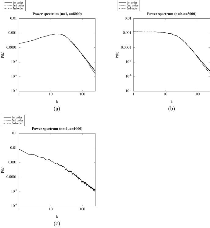
Figure 1: Power spectra of density fluctuation computed from Lagrangian first-, second-, and third-order approximations. (a) The initial spectrum index is $n=1$. The power spectra are at $a=8000$. The difference between the results by the first-, second-, and third-order Lagrangian approximation appears. (b) The power spectra are at $a=3000$ for $n=0$. In this case, the effect of the third-order approximation also appears. (c) The power spectra are at $a=1000$ for $n=-1$. The difference from Lagrangian approximation will still be very small just before shell-crossing.

Fig. 1 shows the power spectra for $n=+1,0,-1$ at $a=8000~{}(n=1)$, $a=3000~{}(n=0)$, and $a=1000~{}(n=-1)$. In these figures, we take an ensemble average of 900 samples. For $n=1$ and $n=0$, a difference between the results by the first-, second-, and third-order Lagrangian approximations appears. The effect of the higher-order approximation suppresses the evolution of the density fluctuation. However, for $n=-1$, because the initial power in the large wavenumber component is small, the pressure does not surpress the evolution well. Therefore, the difference between the Lagrangian approximations still be very small even just before shell-crossing.

In the one-dimensional model, the pressure only affects the nonlinear effect. However, in the three-dimensional realistic model, the gravitational force also affects the nonlinear effect, and the difference between first-, second-, and third-order approximation obviously appears. In fact, according to the comparison between the first-order approximation and full-order numerical calculation, the difference becomes large in the strongly nonlinear region Tatekawa04B .

V Summary and Concluding Remarks

In this paper, we showed the third-order Lagrangian perturbative equations for the cosmological fluid with pressure. Then we derived third-order perturbative solutions for a simple case.

In our analysis for a planar model, the effect of the third-order perturbation seems very small even at the nonlinear stage. However, our result does not show that we can ignore the third-order perturbation easily. As mentioned in Sec. IV, when we introduce planar symmetry, the nonlinear term of the gravitational force disappears. When we consider the effect of nonlinear pressure and gravitational force, the third-order perturbation is expected as a powerful tool to treat high-density regions.

Recently several dark matter models have been proposed DarkMatter . If the interaction in some kind of dark matter can be described by the effective pressure, we can examine the behavior of the density fluctuation in a quasi-nonlinear stage. Furthermore, when we compare the observations and the structure that is formed by using the pressure model, we can delimit the nature of the dark matter. Especially when we consider high-density regions, the third-order perturbative solutions may become useful.

Appendix A Second-order equation for spherical symmetric model with pressure

When we consider spherical collapse or expansion of a spherical void, we introduce spherical symmetry.

The second order perturbative equation (Eq. (23)) is changed as follows:

$$\nabla^{2}\left(\ddot{\zeta}+2\frac{\dot{a}}{a}\dot{\zeta}-4\pi G\rho_{b}\zeta-\frac{1}{a^{2}}\frac{{\rm d}P}{{\rm d}\rho}(\rho_{b})\nabla^{2}\zeta\right)$$ (65)

$$= 2\pi G\rho_{b}\left[\frac{-2S^{\prime}(S^{\prime}+2rS^{\prime\prime})}{r^{2}}\right]$$

$$-\frac{{\rm d}P}{{\rm d}\rho}(\rho_{b})\left[\frac{(-2S^{\prime}+2rS^{\prime\prime}+r^{2}S^{\prime\prime\prime})^{2}}{r^{4}}\right.$$

$$~{}~{}~{}~{}\left.+\frac{6(S^{\prime})^{2}-12rS^{\prime}S^{\prime\prime}+6r^{2}(S^{\prime\prime})^{2}+r^{4}(S^{\prime\prime\prime})^{2}}{r^{4}}\right.$$

$$~{}~{}~{}~{}\left.+2\frac{S^{\prime}(-4S^{\prime}+8rS^{\prime\prime}+2r^{2}S^{\prime\prime\prime})+r^{2}S^{\prime\prime}(-4S^{\prime\prime}+2rS^{\prime\prime\prime}+r^{2}S^{\prime\prime\prime\prime})}{r^{4}}\right]$$

$$-\frac{{\rm d}^{2}P}{{\rm d}\rho^{2}}(\rho_{b})\rho_{b}\left[\frac{(4S^{\prime\prime\prime}+rS^{\prime\prime\prime\prime})(2S^{\prime}+rS^{\prime\prime})}{r^{2}}+\frac{(-2S^{\prime}+2rS^{\prime\prime}+r^{2}S^{\prime\prime\prime})^{2}}{r^{4}}\right]$$

$$= -4\pi G\rho_{b}\frac{S^{\prime}(S^{\prime}+2rS^{\prime\prime})}{r^{2}}$$

$$-\frac{1}{r^{4}}\frac{{\rm d}P}{{\rm d}\rho}(\rho_{b})\left[2(S^{\prime})^{2}-4rS^{\prime}S^{\prime\prime}+2r^{2}(S^{\prime\prime})^{2}+8r^{3}S^{\prime\prime}S^{\prime\prime\prime}+2r^{4}((S^{\prime\prime\prime})^{2}+S^{\prime\prime}S^{\prime\prime\prime\prime})\right]$$

$$-\frac{1}{r^{4}}\frac{{\rm d}^{2}P}{{\rm d}\rho^{2}}(\rho_{b})\rho_{b}\left[4(S^{\prime})^{2}-8rS^{\prime}S^{\prime\prime}+4r^{2}((S^{\prime\prime})^{2}+S^{\prime}S^{\prime\prime\prime})+2r^{3}(S^{\prime}S^{\prime\prime\prime\prime}+4S^{\prime\prime}S^{\prime\prime\prime})+r^{4}(S^{\prime\prime}S^{\prime\prime\prime\prime}+(S^{\prime\prime\prime})^{2})\right]\,,$$

where $S$ and $\zeta$ are the first- and the second-order Lagrangian perturbation, respectively. Because the mode-coupling of the first-order perturbation becomes very complicated, it seems very difficult to solve the equation (65).

References

• (1) Ya. B. Zel’dovich, Astron. Astrophys. 5, 84 (1970).
• (2) V. I. Arnol’d, S. F. Shandarin, and Ya. B. Zel’dovich, Geophys. Astrophys. Fluid Dynamics 20, 111 (1982).
• (3) S. F. Shandarin and Ya. B. Zel’dovich, Rev. Mod. Phys. 61, 185 (1989).
• (4) T. Buchert, Astron. Astrophys. 223, 9 (1989).
• (5) P. Coles and F. Lucchin, Cosmology: The Origin and Evolution of Cosmic Structure (John Wiley & Sons, Chichester, 1995).
• (6) V. Sahni and P. Coles, Phys. Rep. 262, 1 (1995).
• (7) D. Munshi, V. Sahni, and A. A. Starobinsky, Astrophys. J. 436, 517 (1994).
• (8) V. Sahni and S. F. Shandarin, Mon. Not. R. Astron. Soc. 282, 641 (1996).
• (9) A. Yoshisato, T. Matsubara, and M. Morikawa, Astrophys. J. 498, 48 (1998).
• (10) J. D. Barrow and P. Saich, Class. Quantum Grav. 10, 79 (1993).
• (11) F. R. Bouchet, R. Juszkiewicz, S. Colombi, and R. Pellat, Astrophys. J. 394, L5 (1992).
• (12) F. R. Bouchet, S. Colombi, E. Hivon, and R. Juszkiewicz, Astron. Astrophys. 296, 575 (1995).
• (13) T. Buchert, Mon. Not. R. Astron. Soc. 254, 729 (1992).
• (14) T. Buchert and J. Ehlers, Mon. Not. R. Astron. Soc. 264, 375 (1993).
• (15) T. Buchert, Mon. Not. R. Astron. Soc. 267, 811 (1994).
• (16) P. Catelan, Mon. Not. R. Astron. Soc. 276, 115 (1995).
• (17) M. Sasaki and M. Kasai, Prog. Theor. Phys. 99, 585 (1998).
• (18) T. Buchert and A. Domínguez, Astron. Astrophys. 335, 395 (1998).
• (19) J. Binney and S. Tremaine, Galactic Dynamics (Princeton University Press, Princeton, NJ, 1987).
• (20) S. Adler and T. Buchert, Astron. Astrophys. 343, 317 (1999).
• (21) M. Morita and T. Tatekawa, Mon. Not. R. Astron. Soc. 328, 815 (2001).
• (22) T. Tatekawa, M. Suda, K. Maeda, M. Morita, and H. Anzai, Phys. Rev. D66, 064014 (2002).
• (23) T. Tatekawa, astro-ph/0412025.
• (24) T. Tatekawa, Phys. Rev. D70, 064010 (2004).
• (25) J. P. Ostriker and P. Steinhardt, Science 300, 1909 (2003).