GRMHD Simulations of Disk/Jet Systems: Application to the Inner Engines of Collapsars

Abstract

We have carried out 2D and 3D general relativistic magnetohydrodynamic simulations of jets launched self-consistently from accretion disks orbiting Kerr black holes and applied the results to the inner engine of the collapsar model of gamma-ray bursts. The accretion flow launches energetic jets in the axial funnel region of the disk/jet system, as well as a substantial coronal wind. The jets feature knot-like structures of extremely hot, ultra-relativistic gas; the gas in these knots begins at moderate velocities near the inner engine, and is accelerated to ultra-relativistic velocities (Lorentz factors of 50, and higher) by the Lorentz force in the axial funnel. The increase in jet velocity takes place in an acceleration zone extending to at least a few hundred gravitational radii from the inner engine. The overall energetics of the jets are strongly spin-dependent, with high-spin black holes producing the highest energy and mass fluxes. In addition, with high-spin black holes, the ultra-relativistic outflow is cylindrically collimated within a few hundred gravitational radii of the black hole, whereas in the zero-spin case the jet retains a constant opening angle of approximately 16 degrees. The simulations also show that the coronal wind, though considerably slower and colder than the jets, also carries a significant amount of mass and energy. When simulation data is scaled to the physical dimensions of a collapsar the jets operate for a period ranging from 0.1 to 1.4 seconds, until the accretion disk is depleted, delivering $10^{48}$ to $10^{49}$ erg. Longer duration and higher energies are inferred for more massive disks. However, the presence of a strong coronal wind has important implications for any remnant stellar fallback material that has not migrated to the main accretion disk before the wind is established; our simulations suggest that such material would be blown out by the coronal wind.

1 Introduction

The numerical study of black hole accretion has been an area of ongoing research, beginning with the pioneering studies of Wilson (1972). Simulations of accretion mediated by the Magneto-Rotational Instability (MRI; Balbus & Hawley, 1998) also have a long history, with various approximations used to mimic the properties of the inner engine (e.g., the pseudo-Newtonian simulations of Hawley & Krolik, 2001). More recently, codes such as the GRMHD code of De Villiers & Hawley (2003; hereafter DH03) have been used to study accretion disks orbiting Kerr black holes and the jets that arise self-consistently from the accretion flow (De Villiers, Hawley & Krolik, 2003; hereafter DHK). The key result from these simulations is that GRMHD is required to correctly capture the effect of black hole spin on the energy of the jets (De Villiers et al., 2005; hereafter D05), which are powered by an MHD interaction between the accretion flow and the spinning black hole.

In this paper, we analyze in greater detail the jets that arise in accretion simulations. We use a new version of the GRMHD code which features an expanded dynamic range, to better handle the large density contrast between disk and jet, as well as a significantly higher upper bound on the Lorentz factor ($W_{\rm max}=$ 50, instead of 8 in the older code, as discussed in the Appendix). Our 2D and 3D simulations follow the evolution of thick accretion tori located close to the marginally stable orbit, $r_{\rm ms}$, of the black hole. This choice of initial conditions is meant to establish whether the basic dynamics of the disk/jet system evolved by the GRMHD code can reproduce the essential features invoked for the inner engine in the collapsar model of gamma-ray bursts (GRBs; Woosley, 1993, hereafter W93). In this scenario, that of failed Type Ib supernovae, the core of Wolf-Rayet star has undergone collapse to a black hole and a thick accretion disk has formed near the marginally stable orbit of the black hole. The accretion flow is thought to power energetic jets along the rotational axis which are responsible for the release of brief, intense bursts of radiation once the jets reach the optically thin region at the surface of the stellar remnant. Collapsar simulations using a variety of techniques have been reported in the literature: hydrodynamic simulations, e.g. MacFadyen & Woosley (1999); pseudo-Newtonian magnetohydronamic simulations, e.g. Proga et al. (2003), which improve upon hydrodynamic models by better representing the turbulent transport of angular momentum; and more recent attempts to apply GRMHD to the problem, e.g. Mizuno et al. (2003). The simulations reported here consider the dynamics of a long-lived disk/jet system in a self-consistent manner using full GRMHD, allowing us to better quantify the energetics of the system and the role played by black hole spin in the energy of the jets.

Given the ability to simulate the relativistic dynamics of the inner engine of a collapsar, we seek to answer three questions: what is the range of Lorentz factors in the jets; how much energy is transported by these jets (and for how long); and how variable is the flux of energy. The answer to these questions should help to establish whether the dynamics of the GRMHD interaction between disk, black hole, and jet in our numerical setup support the basic tenets of the collapsar model. Since the GRMHD code is scale-free, we will discuss the scaling of our results to the collapsar model in a separate section. We follow the notation used in DH03; a summary of the equations evolved by the GRMHD code and the set of dynamical variables available for analysis is given in the appendix, where a discussion of the numerical determination of the Lorentz factor is also given.

We report all simulation results in geometrodynamic units (Misner, Thorne & Wheeler, 1973), so that time and distance are measured in units of the black hole mass, $M_{\rm BH}$. The GRMHD code uses the test-fluid approximation, so that energy of the orbiting fluid does not alter the background spacetime. We express mass and energy in relation to the maximum initial torus values. The simulation output consists of an extensive collection of data dumps, obtained at increments of $2\,M$ of simulation time; these dumps are used to compute shell-averaged fluxes to measure energy output and temporal variability (see DHK for details).

2 Overview of Disk/Jet Simulations

The initial state of our simulations is similar to that of DHK: a torus with a near-Keplerian rotation profile is seeded with a weak poloidal magnetic field (the strength of the field is set using the ratio of average gas to magnetic pressure in the torus, $\beta_{\rm disk}=\langle P_{\rm gas}\rangle/\langle P_{\rm mag}\rangle=$ 100) to trigger the MRI and generate an accretion flow. As noted above, two important code improvements allow us to probe the dynamics of the axial funnel more thoroughly: an expanded dynamic range and a significantly increased ceiling on the Lorentz factor (now at 50). These improvements are crucial to addressing issues of jet dynamics. Furthermore, to follow the evolution of the jets away from the inner engine, we use a greatly extended radial range (in the 2D simulations). Also, the grid outside the initial torus contains a radially infalling dust (the Bondi solution discussed in Hawley, Smarr & Wilson, 1984; hereafter HSW) to provide an influx of matter against which the emerging jets must compete. The density contrast between dust and torus, at $10^{-6}$ (see Table 1), was chosen to be larger than the typical value of a collapsar environment (W93) for reasons that will be touched upon in the following sections. In some simulations, this torus is also embedded in an external vertical magnetic field (Wald, 1974; hereafter W74) to gain insights into the possible effects of such ambient fields. The strength of these fields was chosen so that they could potentially interact with the MRI-generated fields, as measured by $\beta_{\rm dust}$, the ratio of gas to magnetic pressure outside the initial torus. The choice of initial strength (see Table 1) was established in tests which revealed that strong fields tended to disrupt the initial torus through magnetic tension; “intermediate” values were chosen for these simulations.

The set of simulations consists of 6 models: the S (Schwarzschild, specific angular momentum $a/M=$ 0), R (Rapidly rotating Kerr hole, $a/M=$ 0.9), and E (Extreme Kerr hole, $a/M=$ 0.995) models, with or without an external vertical field (distinguished by the subscript “vf”, e.g., models E and ${\rm E}_{\rm vf}$). As shown in Table 1, the structural parameters of the initial tori place the initial pressure maximum close to the black hole; this approximates collapsar initial conditions (W93) and also provides a rapid evolution since the MRI which drives accretion operates on the orbital time scale of the initial torus, $T_{\rm orb}/M\approx$ 400. Simulations follow the evolution of the accretion disk through 5 orbits ($t_{\rm max}/M=$ 2000) for models R and E, and roughly 8 orbits for the S models. We also carried out one 3D simulation analogous to model ${\rm R}_{\rm vf}$, though with a smaller radial extent. Such a simulation is important to shed light on possible artifacts due to axisymmetry.

The data collection interval, which begins at $t/M=$ 1200 for the high-spin models ($t/M=$ 2400 for Schwarzschild) and extends for two full orbits of the main accretion disk. The start of the interval is chosen to avoid the early transient stage when the initial torus transforms into a turbulent accretion disk; the mass and energy fluxes during this transient phase would generate highly misleading results. After the transient phase, the accretion disk enters a quasi-steady state where the MRI-driven turbulence transports angular momentum outward, and accretion and ejection also proceed in a sustained manner. Extending the data gathering interval for two orbits ensures that representative time-averaged fluxes are obtained.

3 Simulation Results

The broad features of the simulations are similar to those discussed in DHK and D05: the formation of a turbulent accretion flow after roughly two orbits of the main torus and the emergence of an evacuated funnel containing an unbound outflow driven by a largely radial magnetic field. An extensive unbound coronal wind occupies the space between the main accretion disk and the funnel outflow. We use specific binding energy, $e_{\rm bind}=-h\,U_{t}$, to distinguish the jet ($e_{\rm bind}>1.5$) from the unbound coronal outflow ($1.5\geq e_{\rm bind}\geq 1$) and the main disk ($e_{\rm bind}<1$). Jets launched by a rapidly spinning black hole ($a/M=$ 0.9, 0.995) are energetic; those launched by a non-rotating hole are considerably weaker. The jets have a two-component structure: a hot, fast, tenuous outflow in the funnel proper, and a slower, colder, massive jet along the funnel wall. The funnel-wall jets are episodic in nature, fed by injection events where the accretion flow, corona, and funnel converge, at a radial distance comparable to the marginally stable orbit, $r_{\rm ms}$. The most significant difference between the S models and the high-spin models is that jet material in the S models is much slower to reach the outer radial boundary (hence the extended simulation time). Animations of gas density show that the 2D R- and E-model jets have displaced the initial radially infalling gas from the funnel by $t/M\approx$ 1200, whereas the S-model jets only do so by $t/M\approx$ 2400.

3.1 Jet Launching Mechanism

The mechanism by which jets are launched was discussed in D05; the following summary reiterates the salient points of the complex dynamics by which unbound outflows emerge from the accretion flow. In the region of the accretion flow near the marginally stable orbit (the inner torus region in the terminology of DHK), both pressure gradients and the Lorentz force act to lift material away from the equatorial plane. Some of this material is launched magneto-centrifugally in a manner reminiscent of the scenario of Blandford & Payne (1982), generating the coronal wind; some of this material, which has too much angular momentum to penetrate the centrifugal barrier, also becomes part of the massive funnel-wall jet. There is also evidence that the low-angular momentum funnel outflow originates deeper in the accretion flow. Some of this material is produced in a gravitohydromagnetic (GHM) interaction in the ergosphere (Punsly & Coroniti, 1990; Punsly, 2005), and possibly in a process similar to that proposed by Blandford & Znajek (1977) where conditions in the ergosphere approach the force-free limit. The material in the funnel outflow is accelerated by a relatively strong, predominantly radial Lorentz force; gas pressure gradients in the funnel do not contribute significantly. There is also a significant amount of entrainment at the interface between the funnel wall and corona.

3.2 Lorentz Factor and Enthalpy Knots

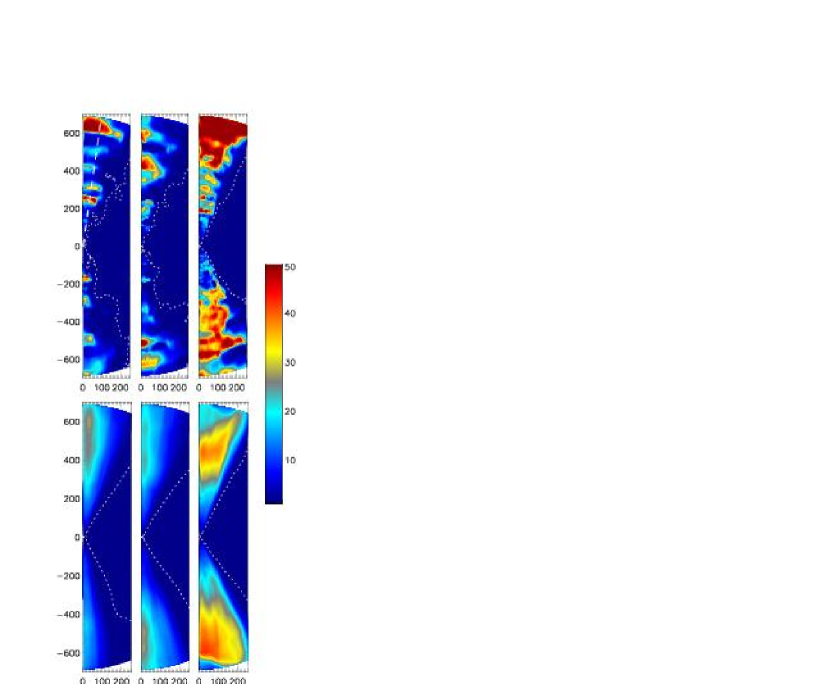
Figure 1: Lorentz factor, $W$, in the funnel outflow. In all panels, the axes are in units of $M$ ($1\,M\approx 4$ km scaled to collapsar dimensions). The black hole is located at the origin. The top row, left to right, shows plots of $W(r,\theta)$ for models ${\rm E}_{\rm vf}$ and ${\rm R}_{\rm vf}$ at $t/M=$ 2000M, and ${\rm S}_{\rm vf}$ at $t/M=$ 3200. The dotted contour corresponds to $e_{\rm bind}=1.5$ and marks the boundary of the jets. The only region where elevated values of $W$ are found is in the jets (and also in the bound plunging inflow near the black hole, which is not resolved at the scale of this figure). Maximum values of $W$ are found in knots that appear episodically in the upper and lower parts of the funnel. The bottom three panels show, from left to right, the time-averaged value of the Lorentz factor, $\langle W(r,\theta)\rangle_{t}$, for models ${\rm E}_{\rm vf}$ and ${\rm R}_{\rm vf}$ ($1200\,M\leq t\leq 2000\,M$), and ${\rm S}_{\rm vf}$ ($2400\,M\leq t\leq 3200\,M$). These plots show evidence of an extended acceleration zone: large Lorentz factors are built up over the full radial range. The plots also show evidence of spin-dependent collimation: for $r/M\gtrsim 300$, cylindrical collimation is seen in the high-spin models (E,R), while the zero-spin model shows no such collimation. The plots also show a model-dependent asymmetry; this feature does not depend on the presence of an initial vertical field. The dashed line in the top left panel is the line of constant $\theta$ along which the cut shown in Figure 2 was taken.

Turning now to the question of Lorentz factor, $W$, in the funnel outflow, Figure 1 shows $W(r,\theta)$ for the ${\rm E}_{\rm vf}$, ${\rm R}_{\rm vf}$, and ${\rm S}_{\rm vf}$ models at the end of the simulations, as well as time-averaged values, $\langle W(r,\theta)\rangle_{t}$ for each model. Elevated values of the Lorentz factor are found in compact, hot, evacuated knots that ascend the funnel radially; the combination of low density and high temperature in the knots yields high specific enthalpy, $h=1+\epsilon+P/\rho$. The highest values of Lorentz factor reach the maximum allowed by the code ($W_{\rm max}=50$, and test runs show that much higher values could be reached with a higher ceiling [see Appendix]), and these are only found at large radii, suggesting the presence of an extensive region where the knots are gradually accelerated to higher Lorentz factors. The time-averaged plots contain three interesting features: i) maxima at large radii, ii) asymmetry, and iii) spin-dependent collimation.

i) Time-averaging smoothes out the passage of the knots and reinforces the notion of an extensive acceleration zone; the Lorentz factor increases smoothly from the base of the jet, near $r_{\rm ms}$, outward to $r/M\approx$ 400—600, where the maxima are found.

ii) The asymmetry in the north and south components of the jets, which is seen both in the instantaneous and time-averaged plots, depends on the details of injection at the base of the jet and on the time interval for data collection (the dominance of one or the other funnel will reverse in the course of long simulations).

iii) Perhaps the most striking feature of the time-averaged plots is the suggestion of strong cylindrical collimation in the high-spin models; whereas the S model shows a time-averaged pattern with a constant opening angle of approximately 16 degrees, the plots of the high-spin models indicate that the ultra-relativistic components of the jets run roughly parallel to the axis for $r/M\gtrsim$ 300. For the models with no initial vertical field, we find similar patterns for $W(r,\theta)$ and $\langle W(r,\theta)\rangle_{t}$ with one important exception: the maximum values seen in the time-averaged plots are systematically lower where no initial external field is present. Collimation is not enhanced by the initial external field in our simulations; as is the case in the simulations with no initial external field, the properties of the funnel magnetic field are largely determined by the accretion flow (D05).

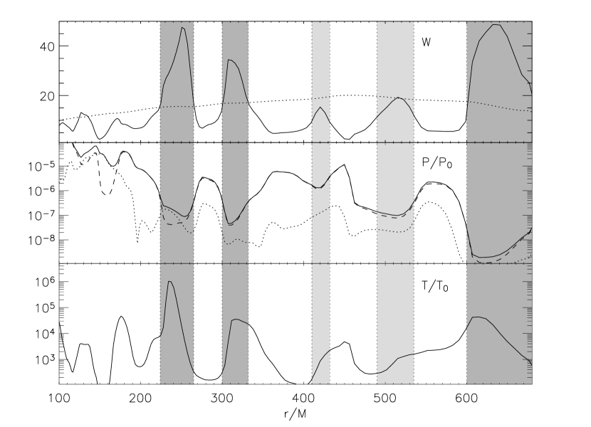
Figure 2: Radial cut through the upper funnel at $t=2000M$ for model ${\rm E}_{\rm vf}$ ($a/M=0.995$; see Figure 1 for location of the cut). The top panel shows the Lorentz factor, $W(r)$, at $t/M=$ 2000 (solid line), and $\langle W(r)\rangle_{t}$ (dotted line). Knots with $W>20$ are shaded in dark gray; knots with $10<W<20$ are shaded lighter gray. The shading is extended to lower panels to help align features in other quantities. The second panel from the top shows pressure (total — solid line, gas — dashed, magnetic — dotted line) scaled to the maximum pressure in the initial torus. The bottom panel shows temperature, scaled to the maximum temperature in the initial torus; the knots with elevated $W$ are $10^{4}$ to $10^{6}$ times hotter than the initial torus.

The dashed line in the top left panel of Figure 1 indicates the angle at which a cut was taken through the knots for model ${\rm E}_{\rm vf}$. Data along this cut is shown in Figure 2. The top panel shows $W(r)$ as a solid line and $\langle W(r)\rangle_{\rm t}$ as a dashed line. The grey shaded regions extending to the lower panels help locate the knots against other code variables. The second panel from the top shows pressure (total, gas, and magnetic), referenced to the initial torus maximum pressure; the knots sit in the troughs of outbound pressure waves. The bottom panel shows temperature, referenced to the initial torus maximum temperature; the knots, which are at least in part heated by shocks, are significantly hotter than the surrounding jet material, and considerably hotter than the initial torus.

3.3 Jet Variability

The jets show a great deal of temporal variability. Figure 3 shows the time dependence of shell-averaged radial mass flux ($\dot{M}=\langle\rho\,U^{r}\rangle$) and energy flux ($\dot{E}=\langle{T^{r}}_{t}\rangle$, including both the dominant fluid enthalpy component and the electromagnetic component) of jet material ($e_{\rm bind}>1.5$) at $r/M=$ 15, near the base of the jet, and at $r/M=$ 100, in the acceleration zone for model ${\rm E}_{\rm vf}$. Close to the black hole, fine structure is detectable at a time scale comparable to the horizon light-crossing time. Energy flux comes in intense bursts corresponding to the passage of knots through the region, followed by extensive quiescent periods. At larger radii, variability follows a similar pattern, but the fine structure tends to be smoothed out by processes taking place higher in the funnel, such as entrainment (D05) and shocks.

3.4 Mass and Energy Flux

Table 2 summarizes the normalized rates of mass ($\dot{M}$) and energy ($\dot{E}$) transported by the jets and coronal wind; these quantities are computed by integrating numerical fluxes through shells at $r/M=$ 100 (to compare 2D and 3D models) and normalized to initial torus mass ($M_{0}$) and energy ($E_{0}$), and hence are in units of inverse simulation time ($M^{-1}$). It is important to emphasize that these calculations are done in a region where the funnel outflow is well established and the numerical ceiling on the Lorentz factor does not come into play.

To account for mass loss from the disk to the black hole, we compute the rate of mass accretion through the inner radial boundary. The mass and energy carried by the jets and coronal wind increase with increasing black hole spin, while the mass accreted onto the black hole decreases with increasing spin, consistent with the findings of D05. However, the energy in the jets is higher than in the analogous models in D05, in part due to initial conditions, but also due to improvements to the GRMHD code’s ability to handle the dynamics of the jets. The mass and energy carried by the jets and coronal wind in 3D model ${\rm R_{vf}}$3D are comparable to the analogous 2D model ${\rm R_{vf}}$; this suggests that the other axisymmetric models are adequately capturing the fluxes of unbound mass and energy. The main difference between the 3D model and its 2D analog is that the jet is slightly more energetic than the coronal wind in 3D, while the situation is reversed in 2D.

4 Comparison to Collapsar Scenario

To extract physical units from the mass and energy fluxes, we use the light-crossing time $t_{\rm lc}=G\,M_{\rm BH}/c^{3}$ and the gravitational length $r_{g}=G\,M_{\rm BH}/c^{2}$ to rescale time and distance measurements. We take collapsar fiducial parameters comparable to those of W93, namely a black hole mass of $M_{\rm BH}=3\,M_{\odot}$ and an initial torus of mass $0.3\,M_{\odot}$, a value consistent with the initial torus parameters and a central density in the range of $10^{11}$—$10^{12}\,{\rm g}\,{\rm cm}^{-3}$.

In 3D simulations, the lifetime of the jets is set by the reservoir of mass in the main disk; as long as turbulence drives the transport of angular momentum, accretion and ejection will continue. In axisymmetry, the MRI which drives accretion is not sustainable, so a premature end to the accretion/ejection process occurs when the MRI subsides (after approximately 10 orbits of the main disk). Nevertheless, we use the mass fluxes ($\dot{M}$) of the axisymmetric models to infer the lifetime of the jets. This lifetime is determined by the depletion of disk mass, i.e. mass carried by the jet and coronal wind (through $r/M$=100 here) and the mass accreted into the black hole. Table 2 lists the jet lifetimes inferred from the simulation data; the values range from 0.1 to 0.2 s for the high-spin simulations to 1.0 to 1.4 s for the zero-spin case. Since the lifetime for model ${\rm R_{vf}}$3D is comparable to its axisymmetric analog, we can infer that jet lifetimes of a few tenths to a few seconds are predicted by these simulations, with longer lifetimes produced by the lower mass fluxes generated by low-spin black holes.

The jet lifetime is used to calculate the energy transported by the jets through the simple relation $E_{\rm total}=t_{\rm eject}\,\dot{E}\,E_{\rm torus}$, where $E_{\rm torus}=0.3\,M_{\odot}\,c^{2}$ is the rest mass of the initial torus. In all simulations, the energy carried by the jets is between $10^{48}$ and $10^{49}$ erg and some fraction of this energy should be converted to radiation once jet material reaches the optically thin outer region of the collapsar. An analogous calculation shows that the coronal wind carries a comparable amount of energy. These energetic coronal winds flow through a much larger surface area than the jets, but their physical effects on the outer layers of the remnant fallback stellar material are likely non-negligible. Our choice of density contrast between initial torus and infalling dust reinforces this observation: the coronal winds had to reverse a substantial influx of material to become established.

5 Summary and Discussion

We have carried out a series of GRMHD simulations of accretion disk/jet systems in the spacetime of Kerr black holes. One of the most significant aspects of these simulations is that the entire accretion/ejection system is evolved in a self-consistent manner from a weakly magnetized initial torus. Our main motivation for this work was to determine what such simulations could say about the inner engine of the canonical collapsar model of $\gamma$-ray bursts (W93). GRBs are energetic explosions thought to originate during the collapse of massive stars; a significant fraction of the rest mass of the progenitor can be released during such bursts. Recent evidence (Sazonov et al., 2004; Soderberg et al., 2004) suggests that the energy liberated in the form of $\gamma$-rays spans a broader range than previously thought, from $10^{47}$ to $10^{51}$ erg. The duration of the bursts also spans a considerable range, in two broad classes: short duration bursts, less than $\sim 2$ s, featuring a hard $\gamma$-ray spectrum, and longer duration bursts $\sim 20$ s, featuring a softer spectrum (e.g. Mészáros, 2002).

The simulations discussed here, which probe the basic dynamics of the disk/black-hole/jet interaction using full GRMHD, suggest that the collapsar scenario favours events at the low end of the distribution of long-duration bursts, on the order of a few seconds. The lifetime of the jets is set by the depletion of disk mass by the jets and a significant coronal wind, as well as by accretion onto the black hole. With a inner engine consisting of a high-spin black hole, and an initial torus of a few tenths of a solar mass, the jets have a lifetime of a few tenths of a second. In addition, the jet material shows a great deal of temporal variability, associated with the passage of knots of shock-heated gas through the funnel. These knots are progressively accelerated to higher Lorentz factors as they ascend the funnel. Results suggest that the Lorentz factor saturates, in a time-averaged sense, to $W\approx$ 30 to 50 at a radius of $r/M\approx$ 500 to 600 (220 to 260 km scaled to collapsar dimensions); however, this saturation may be an artifact of the ceiling on the Lorentz factor ($W_{\rm max}=50$) in the GRMHD code, and true saturation may occur at greater radii. Fendt and Ouyed (2004), using a relativistic MHD wind model, suggest that Lorentz factors on the order of a few hundred to a few thousand are obtainable at $r/M\gtrsim$ 2000.

In the simulations, the energy transported by the jets is approximately $10^{49}$ erg. Since this energy is channeled into ultra-relativistic axial outflows (cylindrically collimated when driven by a high-spin black hole), strong beaming effects are to be expected. Given that the flux of mass and energy in the jets are good indicators of temporal variability in observables, the time-dependence of the fluxes suggests that emissions from the jets should show bursts of activity on the order of a few milliseconds, with slightly longer quiescent periods. Our simulations indicate that the presence of an initial external (vertical) field can enhance some aspects of the jets, such as the maximum time-averaged Lorentz factor in the jets, while leaving other quantities essentially unchanged; in general terms, the magnetic field generated by the MRI is the main driver of the accretion flow and hence the jets, which are fed by magnetized fluid injected at their base from the accretion flow. The time- averaged distribution of Lorentz factor shows a spin-dependent collimation of the ultra-relativistic jet material; in the high-spin simulations, the jets seem to become cylindrically collimated for $r/M\gtrsim$ 300 (130 km scaled to collapsar dimensions).

Based on our simulations, the action of the inner engine in the canonical collapsar model of W93 can only power GRBs at the low end of the distribution of long-duration bursts. However, the collapsar model also envisages feeding the accretion disk over time from the outer layer of a Wolf-Rayet star. Our results show that such a process would be disrupted following the establishment of the strong coronal winds (which can easily displace a considerable amount of infalling dust). Assuming that some remnant material does manage to make its way to the main accretion disk, then the lifetime and total energy of the inner engine could be plausibly extended. However, this finding does not necessarily argue against the collapsar model in explaining extreme duration bursts; as discussed by Toma et al. (2005), the GRBs at the upper end of the distribution for long-duration bursts can be explained as statistical outliers related to observational effects.

It is important to emphasize that these simulations probe only the dynamics of the collapsar model in a fixed background spacetime. More sophisticated treatments should ideally incorporate a dynamical black hole spacetime (especially if more massive accretion disks are to be modeled) as well as self- consistent calculations of radiative transport. Such a code is not yet available; however, it is hoped that some progress can be made at extracting observables from the fluxes reported here by coupling the GRMHD code to a ray tracer and a suitable emission model, which will provide a more complete picture of the time-dependent signals received by distant observers. This work is currently underway, and should be reported in the near future.

Appendix: Equations of GRMHD; Lorentz Factor Calculations

The GRMHD code, described in detail in DH03, is used to study the dynamical properties of a magnetized fluid in the background spacetime of a Kerr black hole by numerically solving the equation of continuity, $\nabla_{\mu}\left(\rho\,U^{\mu}\right)=0$, the energy-momentum conservation law, $\nabla_{\mu}\,T^{\mu\nu}=0$, and the Maxwell’s equations, $\nabla_{\mu}F^{\mu\nu}=4\,\pi\,J^{\nu}$ and $\nabla_{\mu}{}^{*}F^{\mu\nu}=0$, which, in the MHD approximation, reduce to the induction equation $\partial_{\delta}\,F_{\alpha\beta}+\partial_{\alpha}\,F_{\beta\delta}+\partial_{\beta}\,F_{\delta\alpha}=0$. The GRMHD code evolves a set of primitive and secondary code variables directly; these variables were chosen to correspond directly, or through simple relations, to physical variables (e.g. magnetic field, gas density, velocity). This avoids costly calculations to extract physical variables from tensor quantities. In the above expressions, $\rho$ is the density, $U^{\mu}$ the 4-velocity, $T^{\mu\nu}$ the energy-momentum tensor, and $F_{\alpha\beta}$ the electromagnetic field strength tensor. The energy momentum tensor is given by $T^{\mu\nu}=\left[\left(\rho\,h+{\|b\|}^{2}\right)\,U^{\mu}\,U^{\nu}+\left(P+{{\|b\|}^{2}\over 2}\right)\,g^{\mu\nu}-b^{\mu}\,b^{\nu}\right]$ where $h=1+\epsilon+P/\rho$ is the specific enthalpy, with $\epsilon$ the specific internal energy and $P=\rho\,\epsilon\,(\Gamma-1)$ the ideal gas pressure ($\Gamma$ is the adiabatic exponent); ${\|b\|}^{2}=b^{\mu}\,b_{\mu}$ is the magnetic field intensity; and $b^{\mu}={}^{*}F^{\mu\nu}\,U_{\nu}/(4\,\pi)$ is the magnetic field 4-vector. The induction equation is rewritten in terms of the Constrained Transport (CT; Evans & Hawley, 1988) magnetic field variables ${\cal B}^{i}=\epsilon_{ijk}\,F_{jk}$, as $\partial_{t}{\cal B}^{i}-\partial_{j}\left(V^{i}\,{\cal B}^{j}-V^{j}\,{\cal B}^{i}\right)=0$, where $V^{i}=U^{i}/U^{t}$ is the transport velocity, and $U^{t}=W/\alpha$, with $W$ the Lorentz factor. The CT algorithm ensures that the constraint $\partial_{i}{\cal B}^{i}=0$ is satisfied to rounding error. The Kerr metric is expressed in Boyer-Lindquist coordinates, for which ${ds}^{2}=g_{tt}\,{dt}^{2}+2\,g_{t\phi}\,{dt}\,{d\phi}+g_{rr}\,{dr}^{2}+g_{\theta\theta}\,{d\theta}^{2}+g_{\phi\phi}\,{d\phi}^{2}$; $\alpha={(-g^{tt})}^{-1/2}$ is the lapse function.

The 4-velocity is subject to the constraint $U^{\mu}\,U_{\mu}=-1$. Defining the 4-momentum as $S_{\mu}=(\rho\,h\ +{\|b\|}^{2})\,W\,U_{\mu}$, we obtain the equivalent condition $S^{\mu}S_{\mu}=-{(\rho\,h\,W+{\|b\|}^{2}\,W)}^{2}$. In the GRMHD code, the fundamental variables $D=\rho\,W$ and $E=D\,\epsilon$ are used to write $\rho\,h\,W=D+\Gamma\,E$; the spatial components of the 4-momentum are treated as fundamental variables and evolved using the momentum equations (equation (30) of DH03); and the Lorentz factor, $W$, is extracted using the normalization condition at the end of each time step (along with $V^{i}$). It is straightforward to show that the normalization condition yields the following quartic expression for $W$,

$$\eta^{2}+{(1+\xi\,W)}^{2}\,(1-W^{2})=0$$ (1)

where $\eta={\|\tilde{S}\|}/(D+\Gamma\,E)$, $\xi={\|b\|}^{2}/(D+\Gamma\,E)$, and ${\|\tilde{S}\|}^{2}=S_{r}^{2}/g_{rr}+S_{\theta}^{2}/g_{\theta\theta}+S_{\phi}^{2}/g_{\phi\phi}$. In this approach, the solutions for the Lorentz factor span a two-dimensional parameter space, $W(\eta,\xi)$, with $\eta$ analogous to a fluid velocity and $\xi$ analogous to an Alfvén velocity. Using the analytic expression for the physically allowed root of equation (1) provides a significant improvement over the simpler (and faster) calculation used in earlier versions of the GRMHD code. Though costlier from a numerical point of view, this quartic solution significantly raises the maximum allowable value of the Lorentz factor from $W_{\rm max}=$ 8 in the original code to 50 in the current version. This upper bound, which occurs in the limit of $\xi/\eta\gg 1$, is set by rounding error (in double-precision arithmetic $W_{\rm safe}\lesssim 80$, but the more conservative limit of $W_{\rm max}=50$ has been used in the simulations reported here).

Table 1: Model-specific Initial Conditions and Simulation Parameters

Parameter		Schwarzschild (S)	Rapid Kerr (R)	Extreme Kerr (E)
Black hole:
spin	$a/M$	0.000	0.900	0.995
marg. stable orbit	$r_{\rm ms}/M$	6.00	2.32	1.34
Torus:
inner edge	$r_{\rm in}/M$	9.5	9.5	9.5
pressure max.	$r_{\rm{P}_{\rm max}}/M$	16.9	16.1	16.1
outer edge	$r_{\rm out}/M$	31	36	38
maximum height	$H/M$	5	9	10
orb. period (at $r_{\rm{P}_{\rm max}}$)	$T_{\rm orb}/M$	436	422	424
mass	$M_{0}$	0.225	5.32	8.26
rest energy	$E_{0}$	0.219	5.19	8.08
ang. momentum	$L_{0}$	1.07	24.6	38.5
Background:
density contrast	$\bar{\rho}_{\rm dust}/\bar{\rho}_{\rm disk}$	$10^{-6}$	$10^{-6}$	$10^{-6}$
energy contrast	$\bar{\epsilon}_{\rm dust}/\bar{\epsilon}_{\rm disk}$	$10^{-11}$	$10^{-11}$	$10^{-11}$
vertical field	$B_{0}$	$10^{-6}$	$10^{-6}$	$10^{-8}$
	$\beta_{\rm dust}$	$\sim 10^{3}-10^{4}$	$\sim 10^{2}-10^{3}$	$\sim 10^{4}-10^{5}$
Grid:
Inner boundary	$r_{\rm min}/M$	2.10	1.45	1.25
End time	$t_{\rm max}/M$	4000	2000	2000

Table 2: Normalized Mass and Energy Fluxes

Model	S	${\rm S}_{\rm vf}$	R	${\rm R}_{\rm vf}$	${\rm R}_{\rm vf}$3D	E	${\rm E}_{\rm vf}$
Jets (Funnel Outflow):
$\dot{M}\left(\times{10}^{-5}\right)$	0.010	0.009	0.653	0.836	1.302	1.767	1.150
$\dot{E}\left(\times{10}^{-5}\right)$	0.106	0.091	2.880	3.003	4.131	5.906	3.478
Coronal Wind:
$\dot{M}\left(\times{10}^{-5}\right)$	0.041	0.044	6.093	5.108	2.840	11.430	7.265
$\dot{E}\left(\times{10}^{-5}\right)$	0.045	0.049	6.896	5.843	3.243	13.138	8.387
Black hole accretion:
$\dot{M}\left(\times{10}^{-5}\right)$	1.111	0.825	0.011	0.026	0.064	0.008	0.012
Cummulative:
$t_{\rm eject}$ (s)	1.084	1.380	0.214	0.237	0.316	0.109	0.170
$E_{\rm jet}\left(\times{10}^{48}\,{\rm erg}\right)$	0.615	0.782	3.298	3.804	6.961	3.440	3.162
$E_{\rm wind}\left(\times{10}^{48}\,{\rm erg}\right)$	0.262	0.334	7.896	7.400	5.465	7.652	7.626

Note. — Fluxes computed at $r/M=100$ (jet/wind) and at $r=r_{\rm min}$ (accreted mass). Jet component satisfies $e_{\rm bind}>1.5$; coronal wind satisfies $1.5\geq e_{\rm bind}\geq 1.0$. Fluxes are expressed as fractions of initial torus mass and energy: $\dot{M}=\langle\rho\,U^{r}\rangle/\left(M_{0}\,\Delta t\right)$ and $\dot{E}=\langle-{T^{r}}_{t}\rangle/\left(E_{0}\,\Delta t\right)$, where the flux consists of both the dominant fluid enthalpy component and the electromagnetic component). Angle brackets denote integration $\langle{\cal F}\rangle=\int\int\int{{\cal F}\,\sqrt{-g}\,d\theta\,d\phi\,dt}$; $\Delta t$ denotes the interval of integration (1200 to 2000 M for 2D (R, E) models, 2400 to 3200 M for S models, 1200 to 1700 M for ${\rm R}_{\rm vf}$3D). Ejection time is computed using $t_{\rm eject}=t_{\rm M}/\dot{M}_{\rm tot}$ where $\dot{M}_{\rm tot}\equiv\dot{M}_{\rm(r/M=100)}+\dot{M}_{\rm(r=r_{min})}$ represents total mass loss through jets and coronal wind at $r/M=$ 100 and accretion onto the black hole, converted to seconds using the light-crossing time $t_{\rm M}=G\,M\,c^{-3}$. The total energy is computed using $E_{\rm jet/wind}=t_{\rm eject}\,\dot{E}_{\rm jet/wind}\,E_{\rm torus}$ where $E_{\rm torus}=0.3\,M_{\odot}\,c^{2}$ is the initial torus rest mass in erg.

Figure 3: Shell-averaged mass and energy flux in the jets at $r/M=15.0$ (solid line) and at $r/M=100$ (dashed line) for model ${\rm E}_{\rm vf}$ ($a/M=0.995$). The horizontal axis is in units of M (1 M $\approx 10^{-5}$ s, scaled to collapsar dimensions). The plots show that fluctuations occur on the order of the horizon-crossing time near the black hole, and that bursts of elevated readings are followed by extended quiescent periods, on the order 100 horizon-crossing times. At larger radii, the pattern of bursts and quiescent periods persists, but small-scale fluctuations are smoothed out by processes taking place higher in the funnel (e.g. entrainment, shocks). The bursts in these figures correspond to the passage of knots through the funnel.

References

- Balbus & Hawley (1998) Balbus, S. A., & Hawley, J. F. 1998, Rev. Mod. Phys., 70, 1
- Blandford & Znajek (1977) Blandford, R. D. & Znajek, R. 1977, MNRAS, 179, 433
- Blandford & Payne (1982) Blandford, R. D. & Payne, D. 1982, MNRAS, 199, 833
- De Villiers, & Hawley (2003) De Villiers, J. P. & Hawley, J. F. 2003, ApJ, 589, 458 (DH03)
- De Villiers, Hawley, & Krolik (2003) De Villiers, J. P., Hawley, J. F., & Krolik, J. H. 2003, ApJ, 599, 1238 (DHK)
- De Villiers, Hawley, Krolik, & Hirose (2005) De Villiers, J. P., Hawley, J. F., Krolik, J. H., & Hirose, S. 2005, ApJ, 620, in press (D05)
- Fendt & Ouyed (2004) Fendt, Ch. & Ouyed, R., 2004, ApJ, 608, 378
- Hawley & Krolik (2001) Hawley, J. F. & Krolik, J. H., 2001, ApJ, 548, 348
- Hawley, Smarr & Wilson (1984) Hawley, J. F., Smarr, L. L., & Wilson, J. R., 1984, ApJ, 277, 296 (HSW)
- MacFadyen & Woosley (1999) MacFadyen, A. I. & Woosley, S. E., 1999, ApJ, 524, 262
- Mészáros (2002) Mészáros, P., 2002, ARAA, 40, 137
- Mizuno et al. (2004) Mizuno, Y., Yamada, S., Koide, S. & Shibata, K.,, A. I. & Woosley, S. E., 2004, ApJ, 606, 395
- Misner, Thorne, & Wheeler (1973) Misner, C. W., Thorne, K. S., & Wheeler, J. A, 1973, Gravitation (San Francisco: W.H. Freeman)
- Ouyed et at. (1997) Ouyed, R., Pudritz, R. E., & Stone, J. M.1997, Nature, 385, 409
- Proga et al. (2003) Proga, D., MacFadyen, A. I., Armitage, P. J., & Begelman, M. C., 2003, ApJ, 599, L5
- Punsly (2005) Punsly, B., 2005, astro-ph/0505083
- Punsly & Coroniti (1990) Punsly, B., & Coroniti, F. V. 1990, ApJ, 354, 583
- Sazonov et al. (2004) Sazonov, S. Yu., Lutovinov, A. A. & Sunyaev, R. A., 2004, Nature, 430, 646
- Soderberg et al. (2004) Soderberg, A. M., et al., 2004, Nature, 430, 648
- Toma et al. (2005) Toma, K., Yamazaki, R. and Nakamura, T., 2005, ApJ, 620, 835
- Wald (1974) Wald, R. M., 1974, PrD, 10, 1680 (W74)
- Wilson (1972) Wilson, J. R. 1972, ApJ, 173, 431
- Woosley (1993) Woosley, S. E. 1993, ApJ, 405, 273 (W93)