Measuring the Three-Dimensional Structure of Galaxy Clusters. I. Application to a Sample of 25 Clusters.

Abstract

We discuss a method to constrain the intrinsic shapes of galaxy clusters by combining X-Ray and Sunyaev-Zeldovich observations. The method is applied to a sample of $25$ X-Ray selected clusters, with measured Sunyaev-Zeldovich temperature decrements. The sample turns out to be slightly biased, with strongly elongated clusters preferentially aligned along the line of sight. This result demonstrates that X-Ray selected cluster samples may be affected by morphological and orientation effects even if a relatively high threshold signal-to-noise ratio is used to select the sample. A large majority of the clusters in our sample exhibit a marked triaxial structure; the spherical hypothesis is strongly rejected for most sample members. Cooling flow clusters do not show preferentially regular morphologies. We also show that identification of multiple gravitationally-lensed images, together with measurements of the Sunyaev-Zeldovich effect and X-Ray surface brightness, can provide a simultaneous determination of the three-dimensional structure of a cluster, of the Hubble constant, and the cosmological energy density parameters.

1. Introduction

The intrinsic, three-dimensional (hereafter 3-D) shape of clusters of galaxies is an important cosmological probe. The structure of galaxy clusters is sensitive to the mass density in the universe, so knowledge of this structure can help in discriminating between different cosmological models. It has long been clear that the formation epoch of galaxy clusters strongly depends on the matter density parameter of the universe (Richstone et al., 1992). The growth of structure in a high-matter-density universe is expected to continue to the present day, whereas in a low density universe the fraction of recently formed clusters, which are more likely to have substructure, is lower. Therefore, a sub-critical value of the density parameter $\Omega_{\rm M0}$ favors clusters with steeper density profiles and rounder isodensity contours. Less dramatically, a cosmological constant also delays the formation epoch of clusters, favoring the presence of structural irregularity (Suwa et al., 2003).
An accurate knowledge of intrinsic cluster shape is also required to constrain structure formation models via observations of clusters. The asphericity of dark halos affects the inferred central mass density of clusters, the predicted frequency of gravitational arcs, nonlinear clustering (especially high-order clustering statistics) and dynamics of galactic satellites (see Jing & Suto (2002) and references therein).
Asphericity in the gas density distribution of clusters of galaxies is crucial in modeling X-Ray morphologies and in using clusters as cosmological tools. (Inagaki et al., 1995; Cooray, 1998; Sulkanen, 1999). Assumed cluster shape strongly affects absolute distances obtained from X-Ray/Sunyaev-Zeldovich (SZ) measurements, as well as relative distances obtained from baryon fraction constraints  (Allen et al., 2004; Cooray, 1998). Finally, all cluster mass measurements derived from X-Ray and dynamical observations are sensitive to the assumptions about cluster symmetry.
Of course, only the two-dimensional (2-D) projected properties of clusters can be observed. The question of how to deproject observed images is a well-posed inversion problem that has been studied by many authors (Lucy, 1974; Ryden, 1996; Reblinsky, 2000). Since information is lost in the process of projection it is in general impossible to derive the intrinsic 3-D shape of an astronomical object from a single observation. To some extent, however, one can overcome this degeneracy by combining observations in different wavelengths. For example, Zaroubi et al. (1998, 2001) introduced a model-independent method of image deprojection. This inversion method uses X-Ray, radio and weak lensing maps to infer the underlying 3-D structure for an axially symmetric distribution. Reblinsky (2000) proposed a parameter-free algorithm for the deprojection of observed two dimensional cluster images, again using weak lensing, X-Ray surface brightness and SZ imaging. The 3-D gravitational potential was assumed to be axially symmetric and the inclination angle was required as an input parameter. Strategies for determining the orientation have been also discussed. Doré et al. (2001) proposed a method that, with a perturbative approach and with the aid of SZ and weak lensing data, could predict the cluster X-Ray emissivity without resolving the full 3-D structure of the cluster. The degeneracy between the distance to galaxy clusters and the elongation of the cluster along the line of sight (l.o.s.) was thoroughly discussed by Fox & Pen (2002). They introduced a specific method for finding the intrinsic 3-D shape of triaxial cluster and, at the same time, measuring the distance to the cluster corrected for asphericity, so providing an unbiased estimate of the Hubble constant $H_{0}$. Lee & Suto (2004) recently proposed a theoretical method to reconstruct the shape of triaxial dark matter halos using X-Ray and SZ data. The Hubble constant and the projection angle of one principal axis of the cluster on the plane of the sky being independently known, they constructed a numerical algorithm to determine the halo eccentricities and orientation. However, neither Fox & Pen (2002) nor Lee & Suto (2004) apply their method to real data.
In this paper we focus on X-Ray surface brightness observations and SZ temperature decrement measurements. We show how the intrinsic 3-D shape of a cluster of galaxies can be determined through joint analyses of these data, given an assumed cosmology. We constrain the triaxial structure of a sample of observed clusters of galaxies with measured X-Ray and SZ maps. To break the degeneracy between shape and cosmology, we adopt cosmological parameters which have been relatively well-determined from measurements of the cosmic microwave background (CMB) anisotropy, Type Ia supernovae and the spatial distribution of galaxies. We also show how, if multiply-imaging gravitational lens systems are observed, a joint analysis of strong lensing, X-Rays and SZ data allows a determination of both the 3-D shape of a cluster and the geometrical properties of the universe.
The paper is organized as follows. The basic dependencies of cluster X-Ray emission and the SZE on geometry are reviewed in § 2. In § 3, we show how to reconstruct the 3-D cluster structure from these data, presuming cosmological parameters to be known. In passing we note how the addition of suitable strong gravitational lensing data can constrain the cosmological parameters as well, although we do not impose lensing constraints in this paper. We then turn to face the data. Our cluster sample is introduced in § 4, and in § 5, we present 2-D X-Ray surface brightness parameters for each sample member. The triaxial structure of the clusters is then estimated and analyzed in § 6. § 7 is devoted to a summary and discussion of the results. In Appendix A, we provide details on the triaxial ellipsoidal $\beta$-model, used to describe the intra-cluster gas distribution, while Appendix B is devoted to a discussion of the consequences of our assumption of clusters being triaxial ellipsoids aligned along the line of sight. In Appendix C the identifications of multiple sets of images of background galaxies in strong lensing events is discussed. Throughout this paper, unless otherwise stated, we quote errors at the $68.3\%$ confidence level.

2. Multi-Wavelength Approach

In this section, we summarize the relationships between SZ and X-Ray observables, on the one hand, and cluster shape and distance on the other.

2.1. The Sunyaev-Zeldovich Effect

The gravitational potential wells of galaxy clusters contain plasma at temperatures of about $k_{\rm B}T_{\rm e}\approx 8$-$10\ {\rm keV}$. CMB photons that pass through a cluster interact with the energetic electrons of its hot intra-cluster medium (ICM) through inverse Compton scattering, with a probability $\tau\sim 0.01$. This interaction causes a small distortion in the CMB spectrum, known as the Sunyaev-Zeldovich effect (SZE) (Sunyaev & Zeldovich, 1970; Birkinshaw, 1999), which is proportional to the electron pressure integrated along the l.o.s., i.e. to the first power of the plasma density. The measured temperature decrement $\Delta T_{\rm SZ}$ of the CMB is given by:

$$\frac{\Delta T_{\rm SZ}}{T_{\rm CMB}}=f(\nu,T_{\rm e})\frac{\sigma_{\rm T}k_{\rm B}}{m_{\rm e}c^{2}}\int_{\rm l.o.s.}n_{e}T_{\rm e}dl\$$ (1)

where $T_{\rm e}$ is the temperature of the ICM, $k_{\rm B}$ the Boltzmann constant, $T_{\rm CMB}=2.728^{\circ}$K is the temperature of the CMB, $\sigma_{\rm T}$ the Thompson cross section, $m_{\rm e}$ the electron mass, $c$ the speed of light in vacuum and $f(\nu,T_{\rm e})$ accounts for frequency shift and relativistic corrections.
If we assume that the ICM is described by an isothermal triaxial $\beta$-model distribution, substituting Eq. (A10) into (1) with $m=1$, we obtain:

$$\Delta T_{\rm SZ}=\Delta T_{0}\left(1+\frac{\theta_{1}^{2}+e_{\rm proj}^{2}\theta_{2}^{2}}{\theta_{c,\rm proj}^{2}}\right)^{1/2-3\beta/2}$$ (2)

where $\Delta T_{0}$ is the central temperature decrement which includes all the physical constants and the terms resulting from the l.o.s. integration

$$\Delta T_{0} \equiv T_{\rm CMB}f(\nu,T_{\rm e})\frac{\sigma_{\rm T}k_{\rm B}T_{\rm e}}{m_{\rm e}c^{2}}n_{e0}\sqrt{\pi}$$ (3)

$$\times \frac{D_{\rm c}\theta_{\rm c,proj}}{h^{3/4}}\sqrt{\frac{e_{1}e_{2}}{e_{\rm proj}}}g\left(\beta/2\right)$$

with:

$$g(\alpha)\equiv\frac{\Gamma\left[3\alpha-1/2\right]}{\Gamma\left[3\alpha\right]}.$$

$D_{\rm c}$ is the angular diameter distance to the cluster, $\theta_{i}\equiv x_{i,\rm obs}/D_{\rm c}$ is the projected angular position (on the plane of the sky) of the intrinsic orthogonal coordinate $x_{i,\rm obs}$, $h$ is a function of the cluster shape and orientation (Eq. A11), $e_{\rm proj}$ is the axial ratio of the major to the minor axes of the observed projected isophotes and $\theta_{c,\rm proj}$ the projection on the plane of the sky (p.o.s.) of the intrinsic angular core radius (Eq. A12). In a Friedmann-Lemaître-Robertson-Walker universe filled with pressure-less matter and with a cosmological constant, the angular diameter distance between an observer at a redshift $z_{\rm d}$ and a source at $z_{\rm c}$ is:

$$\left.D_{\rm c}\right|_{\rm Cosm}(z_{\rm d},z_{\rm c})=\frac{c}{H_{0}}\frac{1}{1+z_{\rm c}}\frac{1}{|\Omega_{\rm K0}|}{\rm Sinn}\left(\int_{z_{\rm d}}^{z_{\rm c}}\frac{|\Omega_{\rm K0}|}{{\cal E}(z)}dz\right)$$ (4)

with

$${\cal E}(z) \equiv \frac{H(z)}{H_{0}}$$

$$= \sqrt{\Omega_{\rm M0}(1+z)^{3}+\Omega_{\Lambda 0}+\Omega_{\rm K0}(1+z)^{2}}$$

where $H_{0}$, $\Omega_{\rm M0}$ and $\Omega_{\Lambda 0}$ are the Hubble parameter, the normalized energy density of pressure-less matter and the reduced cosmological constant at $z=0$, respectively. $\Omega_{\rm K0}$ is given by $\Omega_{\rm K0}\equiv 1-\Omega_{M0}-\Omega_{\Lambda 0}$, and Sinn is defined as being $\sinh$ when $\Omega_{\rm K0}>0$, $\sin$ when $\Omega_{\rm K0}<0$, and as the identity when $\Omega_{\rm K0}=0$. A more general expression of the angular diameter distance, also accounting for dark energy and inhomogeneity in matter distribution, can be found in Sereno et al. (2001, 2002).

2.2. X-Ray Surface Brightness

Cluster X-Ray emission is due to bremsstrahlung and line radiation resulting from electron-ion collisions; the X-Ray surface brightness $S_{X}$ is proportional to the integral along the l.o.s. of the square of the electron density:

$$S_{X}=\frac{1}{4\pi(1+z_{\rm c})^{4}}\int_{\rm l.o.s.}n_{e}^{2}\Lambda_{eH}dl$$ (6)

where $\Lambda_{eH}$ is the X-Ray cooling function of the ICM in the cluster rest frame. Substituting Eq. (A10) into (6) with $m=2$, we get:

$$S_{X}=S_{X0}\left(1+\frac{\theta_{1}^{2}+e_{\rm proj}^{2}\theta_{2}^{2}}{\theta_{c,\rm proj}^{2}}\right)^{1/2-3\beta}$$ (7)

where the central surface brightness $S_{X0}$ reads:

$$S_{X0}\equiv\frac{\Lambda_{eH}\ \mu_{e}/\mu_{H}}{4\sqrt{\pi}(1+z_{\rm c})^{4}}n_{e0}^{2}\frac{D_{\rm c}\theta_{\rm c,proj}}{h^{3/4}}\sqrt{\frac{e_{1}e_{2}}{e_{\rm proj}}}\ g(\beta)$$ (8)

$\mu$ is the molecular weight given by: $\mu_{i}\equiv\rho/n_{i}m_{p}$.

3. Combining Heterogeneous Data Sets

Here we discuss how 2-D SZE and X-Ray maps of a cluster can be used to constrain its 3-D shape. We follow a parametric approach. We model the cluster using an isothermal, triaxial $\beta$ profile, and adopt a concordance model for the cosmological distance-redshift relationships. Details of the cluster model are given in Appendix A.
This model has long been used to describe the electron distributions of galaxy clusters. It was originally introduced specifically for dynamically relaxed, isothermal clusters (Cavaliere & Fusco-Femiano, 1978), but it was then observed to fit the X-Ray emission of most galaxy clusters reasonably well. A serious drawback of this model is that electron density profiles with extreme axial ratios lead either to unlikely total mass density distributions, i.e. dumbbell shaped clusters, or to regions with unphysical (negative) density. Nevertheless, we believe its extreme versatility makes it a useful tool for our purposes.
For an ellipsoidal distribution, the 3-D shape of a cluster is described by two axis ratios, $e_{1}$ and $e_{2}$, and the orientation of the cluster is fixed by three Euler angles, $\theta_{\rm Eu},\phi_{\rm Eu}$ and $\psi_{\rm Eu}$. As shown in Eqs. (A1, C2), in our model the density profile of a cluster is characterized by three additional parameters: the central density $n_{e0}$, the slope $\beta$ and a core radius, $r_{\rm c3}$. Under the hypothesis of isothermal ICM, a single value, $T_{\rm e}$, characterizes the temperature profile of the cluster. In all, nine parameters describe the cluster.
As discussed in the previous section, the cosmological dependence of the model enters through the luminosity-redshift relationship. For a flat model universe, this relationship is in turn determined by two parameters: the Hubble constant, $H_{0}$, and the matter density $\Omega_{\rm M0}$.
A projected axis ratio, $e_{\rm proj}$, and an orientation angle, $\psi$, characterize a family of ellipses in the p.o.s. derived from the 2-D projection of 3-D ellipsoids. By fitting an elliptical profile to the X-Ray and/or SZE data, these two parameters can (in principle) be measured. Two other observables, the slope $\beta$ of the profile and the projected core radius $\theta_{c,\rm proj}$ can also be determined from data. Two independent geometrical constraints relate 2-D and 3-D quantities (Eqs. A3, A7).
So far we have discussed only quantities derivable from spatial distributions. Besides these, the cluster central electron density and the temperature of the ICM can be inferred from X-Ray observations with sufficient energy resolution. The observed values of the central temperature decrement, $\Delta T_{0}$ in Eq. (3) and of the central surface brightness, $S_{X0}$ in Eq. (8), provide two further constraints. If some assumption is made on the orientation of the cluster, with eight independent equations and eight unknown physical parameters a full determination of the cluster shape can be obtained. If a rotational ellipsoidal morphology is chosen, a lower number of parameters is needed to describe the three-dimensional shape of clusters; in this case no additional assumption on the inclination is required allowing a full determination of the cluster shape and orientation. This case is treated in details in a subsequent paper (Sereno et al., 2004).

3.1. Adding Strong Lensing Data

We wish to point that, even though we do not do so in this work, strong lensing data can be combined with the X-Ray and SZE observations to break the degeneracy between the intrinsic shape of the lensing cluster and the cosmological parameters. If this were done, one could obtain simultaneous constraints on the cluster parameters and on the cosmology.
In particular, each set of strong gravitational images identified in a cluster strongly constrains the mass distribution of the lens. The convergence $k$ depends on the cosmology only through the ratio of distances $D_{\rm cs}/D_{\rm s}$. Therefore $k$ depends only the cosmological density parameters $\Omega_{i}$, and not on the Hubble constant $H_{0}$. The value of $k_{0}$ changes according to the redshift $z_{s}$ of the lensed source. Image systems produced by sources at different redshifts probe independent values of the ratio $D_{\rm cs}/{D_{\rm s}}$.
Each image system provides a constraint on central value of the convergence $k_{0}(z_{\rm s})$ (Eq. C7). In turn, if both the positions and the redshift of a multiple image system are known, each measured value of $k_{0}$ provides, through Eq. (C7), a further independent constraint on the cosmological energy densities. Each multiply-imaged source provides an independent constraint which relates the cosmological parameters $\Omega_{i}$ to the 3-D shape and orientation of the cluster ($h^{3/4}/\sqrt{e_{1}e_{2}}$). With a sufficient number of image systems, then, a measure of both the intrinsic shape and orientation of the cluster and a simultaneous estimate of all cosmological parameters involved can therefore be performed.

3.2. Angular Diameter Distances from X-Ray and SZE Observations for Triaxial Clusters

It is of course well known that the angular diameter distance to a spherically symmetric cluster can be be inferred from microwave decrement and X-Ray data. The angular diameter distance enters the SZE and the X-Ray emission through a characteristic length-scale of the cluster along the l.o.s. SZE and X-Ray emission depend differently on the density of ICM, and therefore also on the assumed cosmology. A joint analysis of SZE measurements and X-Ray imaging observations, together with the assumption of spherical symmetry, thus can yield the distance to the cluster (Birkinshaw, 1999; Reese et al., 2002). Specifically, one can solve Eqs. (3) and (8) for the angular diameter distance $D_{\rm c}$, by eliminating $n_{\rm e0}$.
More generally, for a triaxial cluster the inferred angular diameter distance takes the form:

$$D_{\rm c} = \left.D_{\rm c}\right|_{\rm Exp}\frac{\theta_{\rm c,proj}}{\theta_{\rm c3}}h^{1/2}$$ (9)

$$= \left.D_{\rm c}\right|_{\rm Exp}h^{3/4}\left(\frac{e_{\rm proj}}{e_{1}e_{2}}\right)^{1/2}$$

where $\left.D_{\rm c}\right|_{\rm Exp}$ is an experimental quantity given by:

$$\left.D_{\rm c}\right|_{\rm Exp} = \frac{\Delta T_{0}^{2}}{S_{\rm X0}}\left(\frac{m_{\rm e}c^{2}}{k_{\rm B}T_{e0}}\right)^{2}\frac{g\left(\beta\right)}{g(\beta/2)^{2}\ \theta_{\rm c,proj}}$$ (10)

$$\times \frac{\Lambda_{eH0}\ \mu_{e}/\mu_{H}}{4\pi^{3/2}f(\nu,T_{\rm e})^{2}\ T^{2}_{\rm CMB}\ \sigma_{\rm T}^{2}\ (1+z_{\rm c})^{4}}.$$

Under the assumption of spherical symmetry, the 3-D morphology of the cluster is completely known: $h=e_{1}=e_{2}=1$, $\theta_{\rm Eu}=\varphi_{\rm Eu}=\psi_{\rm Eu}=0$ and the observed major core radius $\theta_{\rm c,proj}$ reduces to $\theta_{\rm c}$. Hence Eq. (9) becomes:

$$D_{\rm c}=\left.D_{\rm c}\right|_{\rm Exp}$$

and the cluster angular diameter distance can therefore be obtained directly from Eq. (10). The standard approach in the past decades has been to take advantage of this possibility to estimate $D_{\rm c}$ under the assumption of spherical symmetry, in order to constrain the underlying cosmology. Since in fact it is also true that $D_{\rm c}=\left.D_{\rm c}\right|_{\rm Cosm}$, through Eq. (4) an estimate of $H_{0}$ can be obtained if $\Omega_{M0}$ and $\Omega_{\Lambda 0}$ are known from independent observations (Birkinshaw, 1999; Reese et al., 2002; Mason et al., 2001).
The same approach clearly cannot be applied when the assumption of spherical symmetry is relaxed and clusters are considered as more general triaxial systems. In this case an estimate of the axis ratios, shape and orientation parameters is required before $D_{\rm c}$ can be computed. Conversely, if $D_{\rm c}$ is known from the redshift and prior knowledge of the cosmology, then the X-Ray and SZE data can be used to constrain the 3-D morphology of the cluster. In this paper we will follow this latter approach. We assume the values of $\Omega_{i}$ and of $H_{0}$ to be known; $\left.D_{\rm c}\right|_{\rm Cosm}$ can be then determined through Eq. (4). We will then use Eq. (9) to infer the 3-D morphology of a sample of galaxy clusters. We believe the cosmological distance scale is now known with sufficient accuracy to warrant our approach. An impressive body of evidence from CMB anisotropy, Type Ia supernovae, galaxy clustering, large-scale structure, and the Ly$\alpha$ forest  (Wang et al., 2000) are consistent with a the picture of a universe with sub-critical cold dark matter energy density and with two-thirds of the critical density being in the form of dark energy. Tegmark et al. (2004) combine the three dimensional power spectrum from over $200,000$ galaxies in the Sloan Digital Sky Survey with the first-year Wilkinson Microwave Anisotropy Probe (WMAP) data (Spergel et al., 2003) to measure cosmological parameters. Their results are consistent with a flat ($\Omega_{\rm K}=0$) cosmological model with $H_{0}=70^{+4}_{-3}\ {\rm km\ s^{-1}\ Mpc^{-1}}$, $\Omega_{\rm M}=0.30{\pm}0.04$ and with a non-zero cosmological constant. Thanks to the high precision to which cosmological parameters are known, we are able to constrain measurements of $\left.D_{\rm c}\right|_{\rm Cosm}$ for the sample objects within a $5\%$ error.

3.3. Cluster Elongation Along the Line of Sight

For the remainder of this paper, we will assume that every cluster is triaxial, with one principal axis aligned along the l.o.s. (see § 3). In Appendix B we show that the magnitude of the systematic error in inferred elongation parameters cause by such assumption is small compared to the uncertainties arising from the observational errors. Such a straightforward assumption also leads to an extremely simple formalism to describe the resulting three-dimensional shape of clusters, reducing the errors caused by the uncertainties in the observational data.

The assumption that the cluster is aligned along the l.o.s. implies: $\theta_{\rm Eu}=\varphi_{\rm Eu}=\psi_{\rm Eu}=0,\ h=1,\ j=e_{1}^{2},\ k=0,\ {\rm and}\ l=e_{2}^{2}$; (see Appendix A). We label axes so that major axis is parallel to the $x_{1}$; then the projected axial ratio and core radius are: $e_{\rm proj}=v_{2}/v_{1}$ and $\theta_{c,\rm proj}=\theta_{\rm c}/v_{1}$. The angular diameter distance becomes:

$$D_{\rm c}=\left.D_{\rm c}\right|_{\rm Cosm}=\left.D_{\rm c}\right|_{\rm Exp}\frac{v_{3}}{v_{1}}.$$ (11)

We now introduce the elongation $e_{\rm l.o.s.}$, defined as the ratio of the radius of the cluster along the l.o.s. to its major axis in the p.o.s.,

$$e_{\rm l.o.s.} \equiv \frac{v_{1}}{v_{3}}$$ (12)

$$= \frac{\left.D_{\rm c}\right|_{\rm Exp}}{\left.D_{\rm c}\right|_{\rm Cosm}(z,H_{0},\Omega_{M})}.$$ (13)

Spherical clusters have the same radius along the l.o.s. and in the p.o.s. and for them $e_{\rm l.o.s.}=1$. Clusters which are instead more or less elongated along the l.o.s. than in the p.o.s. will have values of $e_{\rm l.o.s.}>1$ or $e_{\rm l.o.s.}<1$, respectively.

4. Data sample

We now apply the formalism described in § 3.3 to a sample of galaxy clusters to infer new information about the extent of the clusters along the l.o.s.
We use two samples of clusters for which combined X-Ray and SZ analysis has already been reported. The sample discussed by Reese et al. (2002) consists of $18$ X-Ray selected clusters with $z\geq 0.14$ and $\delta\geq-15\arcdeg$ and $L_{\rm X}(0.1-2.4\ {\rm keV})\geq 5{\times}10^{44}h_{50}^{-2}\ {\rm erg\ s}^{-1}$ and for which high S/N detections of SZE, high-S/N X-Ray imaging and electron temperatures were available. To these we add the sample of Mason et al. (2001), which contains $7$ clusters from X-Ray-flux-limited sample of Ebeling et al. (1996). Details on the completeness of the latter subsample are given by Mason & Myers (2000).
Basic data for our $25$ clusters, including previously published redshift, plasma temperature and microwave decrement information (Reese et al., 2002; Mason et al., 2001) are presented in Table 1.

Table 1Clusters in the Sample

Cluster	$z$	$k_{\rm B}T_{\rm e}$	$\Delta T_{0}$
		(keV)	($\mu K$)
MS 1137.5+6625	$0.784$	$5.7^{+1.3}_{-0.7}$	$-818^{+98}_{-113}$
MS 0451.6-0305	$0.550$	$10.4^{+1.0}_{-0.8}$	$-1431^{+98}_{-105}$
Cl 0016+1609	$0.546$	$7.55^{+0.72}_{-0.58}$	$-1242^{+105}_{-105}$
RXJ1347.5-1145	$0.451$	$9.3^{+0.7}_{-0.6}$	$-3950^{+350}_{-350}$
A 370	$0.374$	$6.6^{+0.7}_{-0.5}$	$-785^{+118}_{-118}$
MS 1358.4+6245	$0.327$	$7.48^{+0.50}_{-0.42}$	$-784^{+90}_{-90}$
A 1995	$0.322$	$8.59^{+0.86}_{-0.67}$	$-1023^{+83}_{-77}$
A 611	$0.288$	$6.6^{+0.6}_{-0.6}$	$-853^{+120}_{-140}$
A 697	$0.282$	$9.8^{+0.7}_{-0.7}$	$-1410^{+160}_{-180}$
A 1835	$0.252$	$8.21^{+0.19}_{-0.17}$	$-2502^{+150}_{-175}$
A 2261	$0.224$	$8.82^{+0.37}_{-0.32}$	$-1697^{+200}_{-200}$
A 773	$0.216$	$9.29^{+0.41}_{-0.36}$	$-1260^{+160}_{-160}$
A 2163	$0.202$	$12.2^{+1.1}_{-0.7}$	$-1900^{+140}_{-140}$
A 520	$0.202$	$8.33^{+0.46}_{-0.40}$	$-662^{+95}_{-95}$
A 1689	$0.183$	$9.66^{+0.22}_{-0.20}$	$-1729^{+105}_{-120}$
A 665	$0.182$	$9.03^{+0.35}_{-0.31}$	$-728^{+150}_{-150}$
A 2218	$0.171$	$7.05^{+0.22}_{-0.21}$	$-731^{+125}_{-100}$
A 1413	$0.142$	$7.54^{+0.17}_{-0.16}$	$-856^{+110}_{-110}$
A 2142	$0.091$	$7.0\pm 0.2$	$-437^{+25}_{-25}$
A 478	$0.088$	$8.0\pm 0.2$	$-375^{+28}_{-28}$
A 1651	$0.084$	$8.4\pm 0.7$	$-247^{+30}_{-30}$
A 401	$0.074$	$6.4\pm 0.2$	$-338^{+20}_{-20}$
A 399	$0.072$	$9.1\pm 0.4$	$-164^{+21}_{-21}$
A 2256	$0.058$	$9.7\pm 0.8$	$-243^{+29}_{-29}$
A 1656	$0.023$	$6.6\pm 0.2$	$-302^{+48}_{-48}$

Note. — Clusters in the sample; their redshift, gas temperature and central temperature decrement.

5. X-Ray Morphology in Two Dimensions

Chandra and XMM observations of clusters in the past few years have shown that in general clusters exhibit elliptical surface brightness maps, and so cannot be spherically symmetric. In order to obtain a uniform set of X-Ray observables for our sample objects, we have re-analyzed archival X-Ray data for each of them. We have used Chandra and/or XMM data for all objects except A 520, for which only ROSAT data are available.
We modeled the emission of all clusters in the $0.3-7.0\ {\rm keV}$ band. Pixel values of all detected point sources were replaced with values interpolated from the surrounding background regions; the CIAO tools wavdetect and dmfilth were used for this purpose.
Using the SHERPA software, we fitted the cluster surface brightness to elliptical 2-D $\beta$-models (see Eq. 7). Results are listed in Table 2. Fitted models from Chandra and XMM observations are roughly consistent.
The 25 clusters have a weighted median projected axis ratio of $e_{\rm proj}=1.24{\pm}0.09$, in very good agreement with the value of $\langle e_{\rm proj}\rangle=1.25{\pm}0.19$ obtained by Mohr et al. (1995) from Einstein data of a lower-redshift sample of 65 objects. Only six of the $25$ clusters have a projection in the p.o.s. close to be circular ($e_{\rm proj}<1.2$).

Table 2Two-Dimensional Analysis

	$x_{\rm c},y_{\rm c}$
Cluster	R.A.	Decl.	$e_{\rm proj}$	$\theta$	$r_{c}$	$\beta$	Satellite
				(deg)	(arcsec)
MS 1137.5+6625	$11\ 40\ 22.3$	$+66\ 08\ 15.3$	$1.113\pm 0.014$	$63.9\pm 1.0$	$11.28\pm 0.55$	$0.58\pm 0.01$	$1$
MS 0451.6-0305	$04\ 54\ 11.4$	$-03\ 00\ 51.3$	$1.307\pm 0.015$	$84.1\pm 1.1$	$45.1\pm 1.2$	$0.88\pm 0.02$	$1$
Cl 0016+1609	$00\ 18\ 33.5$	$+16\ 26\ 12.9$	$1.205\pm 0.013$	$310.8\pm 1.7$	$36.42\pm 0.93$	$0.63\pm 0.01$	$1$
Cl 0016+1609	$00\ 18\ 33.1$	$+16\ 26\ 10.5$	$1.168\pm 0.019$	$314\pm 3$	$39.0\pm 1.1$	$0.65\pm 0.08$	$2$
RXJ1347.5-1145	$13\ 47\ 30.7$	$-11\ 45\ 09.1$	$1.453\pm 0.019$	$21.5\pm 1.0$	$6.36\pm 0.15$	$0.533\pm 0.003$	$1$
A 370	$02\ 39\ 53.3$	$-01\ 34\ 39.0$	$1.564\pm 0.018$	$353.8\pm 0.7$	$50.1\pm 1.8$	$0.52\pm 0.01$	$1$
MS 1358.4+6245	$13\ 59\ 50.7$	$+62\ 31\ 04.1$	$1.325\pm 0.019$	$23.4\pm 1.4$	$14.23\pm 0.49$	$0.526\pm 0.004$	$1$
A 1995	$14\ 52\ 57.9$	$+58\ 02\ 55.8$	$1.242\pm 0.010$	$122.2\pm 1.0$	$45.78\pm 0.88$	$0.73\pm 0.01$	$1$
A 611	$08\ 00\ 56.8$	$+36\ 03\ 23.5$	$1.14\pm 0.05$	$326\pm 9$	$21.84\pm 0.62$	$0.596\pm 0.006$	$1$
A 697	$08\ 42\ 57.6$	$+36\ 21\ 56.8$	$1.334\pm 0.016$	$16.2\pm 1.2$	$54.3\pm 1.7$	$0.64\pm 0.01$	$1$
A 1835	$14\ 01\ 02.0$	$+02\ 52\ 42.9$	$1.225\pm 0.012$	$7.0\pm 1.4$	$8.34\pm 0.14$	$0.511\pm 0.002$	$1$
A 2261	$17\ 22\ 27.1$	$+32\ 07\ 57.4$	$1.022\pm 0.017$	$0.0\pm 1.7$	$20.58\pm 0.75$	$0.578\pm 0.007$	$1$
A 773	$09\ 17\ 53.1$	$+51\ 43\ 37.9$	$1.237\pm 0.022$	$0.0\pm 2.5$	$49.5\pm 1.9$	$0.63\pm 0.02$	$1$
A 773	$09\ 17\ 52.7$	$+51\ 43\ 37.0$	$1.184\pm 0.019$	$0.0\pm 2.9$	$45.2\pm 2.3$	$0.58\pm 0.06$	$2$
A 2163	$16\ 15\ 46.6$	$-06\ 08\ 44.9$	$1.206\pm 0.004$	$0.0\pm 0.6$	$94.80\pm 0.95$	$0.720\pm 0.005$	$1$
A 2163	$16\ 15\ 46.0$	$-06\ 08\ 46.9$	$1.163\pm 0.009$	$0.0\pm 1.4$	$91.3\pm 1.3$	$0.71\pm 0.01$	$2$
A 520	$04\ 54\ 09.8$	$+02\ 55\ 22.4$	$1.06\pm 0.05$	$347\pm 20$	$115.2\pm 11.8$	$0.59\pm 0.04$	$3$
A 1689	$13\ 11\ 29.6$	$-01\ 20\ 28.0$	$1.141\pm 0.012$	$342.4\pm 2.2$	$27.01\pm 0.73$	$0.582\pm 0.005$	$1$
A 665	$08\ 30\ 57.1$	$+65\ 51\ 01.8$	$1.238\pm 0.012$	$33.7\pm 1.2$	$63.0\pm 1.3$	$0.582\pm 0.006$	$1$
A 2218	$16\ 35\ 51.9$	$+66\ 12\ 34.6$	$1.162\pm 0.009$	$83.5\pm 1.5$	$56.0\pm 0.84$	$0.591\pm 0.004$	$1$
A 2218	$16\ 35\ 52.4$	$+66\ 12\ 33.5$	$1.201\pm 0.013$	$85.4\pm 1.7$	$58.5\pm 1.1$	$0.603\pm 0.009$	$2$
A 1413	$11\ 55\ 17.9$	$+23\ 24\ 16.2$	$1.473\pm 0.019$	$182.2\pm 0.9$	$43.0\pm 1.4$	$0.573\pm 0.007$	$1$
A 2142	$15\ 58\ 20.1$	$+27\ 14\ 03.5$	$1.540\pm 0.007$	$52.3\pm 0.3$	$73.1\pm 1.1$	$0.598\pm 0.005$	$1$
A 478	$04\ 13\ 25.3$	$+10\ 27\ 53.5$	$1.477\pm 0.006$	$43.5\pm 0.3$	$30.53\pm 0.16$	$0.533\pm 0.001$	$1$
A 1651	$12\ 59\ 21.9$	$-04\ 11\ 44.6$	$1.184\pm 0.013$	$272.4\pm 1.9$	$73.4\pm 2.0$	$0.598\pm 0.007$	$1$
A 401	$02\ 58\ 57.1$	$+13\ 34\ 37.8$	$1.303\pm 0.008$	$325.1\pm 0.6$	$142.8\pm 3.0$	$0.625\pm 0.007$	$1$
A 399	$02\ 57\ 52.0$	$+13\ 02\ 38.7$	$1.207\pm 0.009$	$337.5\pm 1.2$	$139.8\pm 3.8$	$0.536\pm 0.008$	$2$
A 2256	$17\ 04\ 00.4$	$+78\ 38\ 37.1$	$1.327\pm 0.008$	$61.3\pm 0.5$	$529\pm 16$	$1.33\pm 0.06$	$2$
A 1656	$12\ 59\ 44.1$	$+27\ 56\ 43.0$	$1.141\pm 0.006$	$0.0\pm 0.6$	$540\pm 34$	$0.65\pm 0.07$	$2$

Note. — Fit parameters of the elliptical $\beta$ model: $x_{\rm c},y_{\rm c}$ is the central position; $e_{proj}$ is the projected axial ratio; $\theta$ is the orientation angle (north over east); $r_{c}$ and $\beta$ are the model core radius and slope, respectively. In the last column, label $1$ is for Chandra, $2$ for XMM and $3$ for ROSAT HRI observation.

5.1. Circular Versus Elliptical $\beta$ Models

Although clusters are rarely circular in projection, some previous joint analyses of X-Ray and SZE data have assumed spherical symmetry. In order to bound the effects of this simplification, we have also modeled the surface brightness profiles of each sample cluster with a circular $\beta$-model. The choice of circular rather than elliptical $\beta$ model does not affect the resulting of the central surface brightness, as shown in the top panel in Fig. 1. For a few clusters the fitted value of the slope $\beta$ differs slightly between circular and elliptical models (middle panel of Fig. 1). As would be expected, however, significantly different values for the core radius are obtained with these two models (bottom panel of Fig.  1). This behavior has already been noted by Hughes & Birkinshaw (1998).
Therefore, relaxing the assumption of circular projection on the p.o.s. when measuring the angular diameter distance (Eq. 10), mainly affects the value of the projected core radius $\theta_{c,\rm proj}$. The bottom panel in Fig. 1 shows that the core radius obtained using a circular $\beta$-model ($\theta_{c,\rm Circ}$) is consistently lower (black squares) than that obtained from an elliptical model ($\theta_{c,\rm Ell}$). $\theta_{c,\rm Circ}$ can in fact be well approximated by the arithmetic mean of the two semi-axes of the elliptical isophotes in the p.o.s.
The angular diameter distance obtained assuming spherical symmetry (Table 3) can therefore, in first approximation, be corrected for the observed ellipticity of the cluster in the p.o.s. multiplying $\left.D_{\rm c}\right|_{\rm Exp}^{\rm Circ}$ by the correction factor $f_{\rm cor}$:

$$\left.D_{\rm c}\right|_{\rm Exp}^{\rm Circ,Corr}=\left.D_{\rm c}\right|_{\rm Exp}^{\rm Circ}f_{\rm cor}=\left.D_{\rm c}\right|_{\rm Exp}^{\rm Circ}\frac{1+e_{\rm proj}}{2e_{\rm proj}}.$$ (14)

As shown in the bottom panel of Fig. 1, the corrected values of the core radii $\left.\theta_{\rm c}\right|_{\rm Circ}^{\rm Cor}$

$$\left.\theta_{\rm c}\right|_{\rm Circ}^{\rm Cor}=\theta_{c,\rm Circ}\ \frac{1}{f_{\rm cor}}$$ (15)

provide a good approximation to $\theta_{c,\rm ell}$ (gray squares).

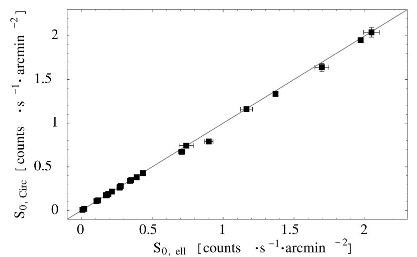
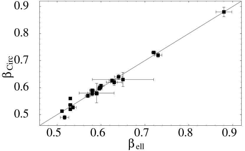
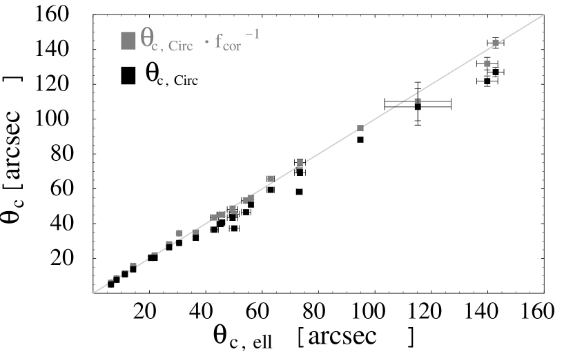
Figure 1.— Comparison of central surface brightness (top), slope $\beta$ (middle) and core radius (bottom) obtained fitting circular and elliptical $\beta$-models to the X-Ray surface brightness maps of sample clusters. In the bottom panel the gray symbols show core radii corrected for the ellipticity as in Eq. 15.

6. Cluster Morphology in Three Dimensions

6.1. Angular Diameter Distances

In order to estimate the l.o.s. extent of clusters, then, we need only to obtain values of $\left.D_{\rm c}\right|_{\rm Exp}$ from the X-Ray and SZE data (via Eq. 10) and compare them (via Eq. 13) to the angular size distance obtained from the measured redshift and our adopted cosmological model. Since only the X-Ray data are publically available, however, we are unable to jointly fit both SZE and X-Ray data. For this reason we must rely on published values of central CMB temperature decrement ($\Delta T_{0}$) for our analysis.
A potential difficulty with this approach is that the available values of $\Delta T_{0}$, from Reese et al. (2002) and Mason et al. (2001), have been inferred assuming that clusters are circularly symmetric when seen in projection on the sky. While this assumption is quite reasonable given the limited spatial resolution of the data available to these authors, it is not, in general, consistent with the results of our analysis of higher-resolution X-Ray data (see Table 2). In the limit of very high spatial resolution SZE data, we would expect this inconsistency to have negligible effect on our results, just as we find that with high-resolution X-Ray data, the same central X-Ray surface brightness is inferred from fits of circular and elliptical models (see the top panel in Fig. 1).
We have computed values of the angular diameter distances for all clusters in the sample both under the assumption of spherical symmetry, and relaxing the assumption to a more general triaxial morphology. For the spherical case results obtained modeling the cluster X-Ray surface brightness profiles with circular $\beta$-models (§ 5.1) were substituted into Eq. (10). For the triaxial case results from the elliptical $\beta$-models were instead used (§ 5). The term $f(\nu,T_{e})$, which accounts for the frequency shift and also includes relativistic corrections, was computed as described by Itoh et al. (1998). Central values of the CMB temperature decrement ($\Delta T_{0}$) were taken from Reese et al. (2002) and Mason et al. (2001). The resulting values of $\left.D_{\rm c}\right|_{\rm Exp}^{\rm Ell}$ are listed in Table 3. The largest source of error (about $70\%$ of the total) is the uncertainty on the SZE measurement of $\Delta T_{0}$. The second most significant error source is the uncertainty in the X-Ray measurement of the intra-cluster plasma temperature (about $20\%$). Both $\left.D_{\rm c}\right|_{\rm Exp}^{\rm Ell}$ and $\left.D_{\rm c}\right|_{\rm Exp}^{\rm Circ}$ are plotted in Fig. 2. A comparison between the experimental quantities $\left.D_{\rm c}\right|_{\rm Exp}^{\rm Circ}$ and $\left.D_{\rm c}\right|_{\rm Exp}^{\rm Ell}$ and the values of $\left.D_{\rm c}\right|_{\rm Cosm}$, together with their relative errors, highlights the high precision to which the cosmological angular distance is known, compared to the two experimental estimates, in support of our approach of a fixed cosmological model.

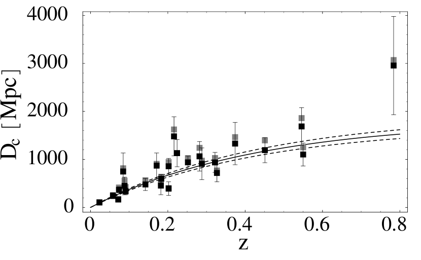
Figure 2.— $\left.D_{\rm c}\right|_{\rm Cosm}$ as a function of redshift (solid line); dashed lines represent the 1$\sigma$ confidence level. Black and grey point represent $\left.D_{\rm c}\right|_{\rm Exp}^{\rm Ell}$ and $\left.D_{\rm c}\right|_{\rm Exp}^{\rm Circ}$ computed in this work, respectively.

Table 3Angular Diameter Distance

Cluster	$\left.D_{\rm c}\right|_{\rm Cosm}$	$\left.D_{\rm c}\right|_{\rm Exp}^{\rm Circ}$	$\left.D_{\rm c}\right|_{\rm Exp}^{\rm Ell}$
	(Mpc)	(Mpc)	(Mpc)
MS 1137.5+6625	$1537^{+71}_{-91}$	$3179^{+1103}_{-1640}$	$2479\pm 1023$
MS 0451.6-0305	$1322^{+58}_{-76}$	$1278^{+265}_{-299}$	$1073\pm 238$
Cl 0016+1609	$1318^{+58}_{-76}$	$2041^{+484}_{-514}$	$1635\pm 391$
RXJ1347.5-1145	$1189^{+52}_{-68}$	$1221^{+368}_{-343}$	$1166\pm 262$
A 370	$1063^{+46}_{-61}$	$4352^{+1388}_{-1245}$	$1231\pm 441$
MS 1358.4+6245	$974^{+41}_{-55}$	$866^{+248}_{-310}$	$697\pm 183$
A 1995	$964^{+41}_{-54}$	$1119^{+247}_{-282}$	$885\pm 207$
A 611	$893^{+38}_{-50}$	$995^{+325}_{-293}$	$934\pm 331$
A 697	$880^{+37}_{-49}$	$998^{+298}_{-250}$	$1099\pm 308$
A 1835	$811^{+37}_{-45}$	$1027^{+194}_{-198}$	$946\pm 131$
A 2261	$743^{+31}_{-41}$	$1049^{+306}_{-272}$	$1118\pm 283$
A 773	$722^{+30}_{-40}$	$1450^{+361}_{-332}$	$1465\pm 407$
A 2163	$686^{+29}_{-38}$	$828^{+181}_{-205}$	$806\pm 163$
A 520	$686^{+29}_{-38}$	$723^{+270}_{-236}$	$387\pm 141$
A 1689	$634^{+27}_{-35}$	$688^{+172}_{-163}$	$604\pm 84$
A 665	$632^{+26}_{-35}$	$466^{+217}_{-179}$	$451\pm 189$
A 2218	$601^{+25}_{-33}$	$1029^{+339}_{-352}$	$809\pm 263$
A 1413	$515^{+21}_{-29}$	$573^{+171}_{-151}$	$478\pm 126$
A 2142	$349^{+14}_{-19}$	$187^{+212}_{-97}$	$335\pm 70$
A 478	$340^{+14}_{-19}$	$406^{+237}_{-135}$	$448\pm 185$
A 1651	$327^{+14}_{-18}$	$373^{+202}_{-122}$	$749\pm 385$
A 401	$289^{+12}_{-16}$	$610^{+593}_{-254}$	$369\pm 62$
A 399	$282^{+12}_{-16}$	$107^{+85}_{-41}$	$165\pm 45$
A 2256	$232^{+10}_{-13}$	$296^{+127}_{-90}$	$242\pm 61$
A 1656	$96^{+4}_{-5}$	$235^{+218}_{-98}$	$103\pm 42$

Note. — Cosmological angular diameter distance, its experimental estimate as reported by Reese et al. (2002) and  Mason et al. (2001) assuming spherical symmetry, and the experimental quantity $\left.D_{\rm c}\right|_{\rm Exp}^{\rm Ell}$, defined by Eq. (10), computed in this paper assuming the clusters are oblate spheroids.

6.2. Elongation Along the Line of Sight

Assuming a general triaxial morphology, the ratio between $\left.D_{\rm c}\right|_{\rm Exp}^{\rm Ell}$ and $\left.D_{\rm c}\right|_{\rm Cosm}$ provides an estimate of the ratio of the cluster axis along the l.o.s. and the cluster major axis in the p.o.s. We have computed values of $\left.D_{\rm c}\right|_{\rm Exp}^{\rm Ell}$ for all clusters in the sample (§ 6.1). For each cluster we have then also computed $\left.D_{\rm c}\right|_{\rm Cosm}$ (Eq. 4) and have then estimated their $e_{\rm l.o.s.}$. Resulting values are listed in Table 4.
Since the observables in our analysis have asymmetric uncertainties, we apply corrections given by D’Agostini (2004) to obtain estimates of sample mean and standard deviation.
All clusters in our sample were X-Ray selected; X-Ray surveys are surface brightness limited. Clusters close to the detection limit which are elongated along the l.o.s. will be detected, while the ones which are more extended in the p.o.s. will be missed. If a surface brightness limit is fixed which is far above the detection limit of the survey, the problem should be eliminated.
In both the Reese et al. (2002) and the Mason et al. (2001) samples this “correction” limit was applied. Our final sample shows in fact only mild signs of preferential elongation of the clusters along the l.o.s. (see Fig. 3). Of the $25$ clusters, $15$ clusters are in fact more elongated along the l.o.s ($e_{\rm l.o.s.}>1$), while the remaining $10$ clusters are compressed. The mean of the distribution of the elongations is $\langle e_{\rm l.o.s.}\rangle=1.15{\pm}0.08$. In presence of likely outliers, the median is a more stable estimator (Gott et al., 2001). The median of the $e_{\rm l.o.s.}$’s is $1.08\pm 0.17$. While on average we observe only a very slight preferential elongation of the clusters along the l.o.s., residual of X-Ray selection effects, clusters with extreme axes ratios are still preferentially selected if the elongation lies along the l.o.s. This is a clear example of how deeply X-Ray selected cluster samples are affected by morphological and orientation issues.

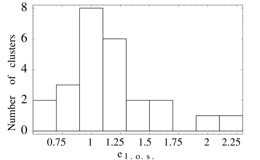
Figure 3.— Distribution of elongation along the l.o.s. for all clusters in our sample.

Table 43-D Morphology

Cluster	$e_{\rm l.o.s.}$	qmax
MS 1137.5+6625	$1.61\pm{0.69}$	$1.79\pm{0.68}$
MS 0451.6-0305	$0.81\pm{0.18}$	$1.31\pm{0.11}$
Cl 0016+1609	$1.24\pm{0.30}$	$1.49\pm{0.32}$
RXJ1347.5-1145	$0.98\pm{0.22}$	$1.45\pm{0.19}$
A 370	$1.16\pm{0.42}$	$1.81\pm{0.48}$
MS 1358.4+6245	$0.72\pm{0.19}$	$1.40\pm{0.12}$
A 1995	$0.92\pm{0.21}$	$1.24\pm{0.14}$
A 611	$1.05\pm{0.37}$	$1.19\pm{0.27}$
A 697	$1.25\pm{0.35}$	$1.67\pm{0.40}$
A 1835	$1.17\pm{0.16}$	$1.43\pm{0.18}$
A 2261	$1.51\pm{0.38}$	$1.54\pm{0.39}$
A 773	$2.03\pm{0.56}$	$2.51\pm{0.71}$
A 2163	$1.18\pm{0.24}$	$1.37\pm{0.23}$
A 520	$0.56\pm{0.20}$	$1.77\pm{0.26}$
A 1689	$0.95\pm{0.13}$	$1.14\pm{0.08}$
A 665	$0.71\pm{0.30}$	$1.40\pm{0.29}$
A 2218	$1.85\pm{0.44}$	$1.57\pm{0.45}$
A 1413	$0.93\pm{0.25}$	$1.47\pm{0.20}$
A 2142	$0.96\pm{0.20}$	$1.54\pm{0.18}$
A 478	$1.32\pm{0.54}$	$1.95\pm{0.65}$
A 1651	$2.29\pm{1.18}$	$2.71\pm{1.39}$
A 401	$1.28\pm{0.21}$	$1.67\pm{0.27}$
A 399	$0.58\pm{0.16}$	$1.71\pm{0.12}$
A 2256	$1.04\pm{0.26}$	$1.38\pm{0.22}$
A 1656	$1.08\pm{0.43}$	$1.23\pm{0.32}$

Note. — Cluster elongation along the l.o.s. and maximum axial ratio.

6.3. Maximum Axis Ratio

We can estimate the three ellipsoidal axis lengths ($v_{1}$, $v_{2}$ and $v_{3}$ ) from the measured values of $e_{\rm l.o.s.}$ and $e_{\rm proj}$, and from these the ratio of the semi-major to the semi-minor axis, $q_{\rm max}$. $q_{\rm max}$ is an extremely convenient tool to describe the intrinsic shape of a cluster since it allows, without the aid of further parameters, to quantify how far a cluster is from spherical symmetry. For most clusters in the sample, the confidence regions of $v_{1}$, $v_{2}$ and $v_{3}$ are highly overlapping so that, for example, the upper bound of the 1-$\sigma$ interval for the estimate of the ratio between the median and the minor axis, $q_{\rm mid}$, may be larger than the upper limit of $q_{\rm max}$.
To obtain well defined estimates of the errors of the maximum, intermediate and minimum axis ratios for each cluster, assuming the $v_{i}$’s to be normally distributed, we have obtained $10^{5}$ random samples from each distribution. We have then selected the maximum, the intermediate and the minimum values of each set of three in order to build the distribution of the maximum, intermediate and minimum axis ratios. We have finally computed the standard deviations of such three distributions, that provide estimates for the errors for the axes ratios. The resulting values of $q_{max}$ are listed in Table 4 and their distribution is shown in Fig. 4.
$q_{\rm max}$ has a mean value of $\langle q_{\rm max}\rangle=1.59{\pm}0.07$, and a median of $1.49\pm 0.17$. This result is consistent with cosmological simulations in which the mean value of the maximum axial ratio ranges from $1.56$ (Suwa et al., 2003; Kasun & Evrard, 2004) to $1.8$ (Jing & Suto, 2002). The intermediate axis ratios, $q_{\rm mid}$ show a median of $1.21\pm 0.12$. At $1-\sigma$ no cluster in the sample can be approximated as spherical; $11$ clusters are spherical at the $3-\sigma$ confidence level.
Although our estimates are affected by large errors and the data sample is of modest size, we look for trends in the distribution of the maximum axial ratios.
No correlation is observed between the maximum axial ratio and redshift (see Fig. 5 where the solid and dashed lines represent the weighted and non weighted linear best fit to the data, respectively).
A poor correlation is observed also between the maximum axial ratio and the cluster gas temperature. We find at most a weak tendency for hotter clusters to exhibit smaller values of $q_{max}$. The linear weighted best fit to the data is: $q_{\rm max}=(2.02{\pm}0.35)-(0.060{\pm}0.041)\ T$. The trend is plotted in Fig. 6, where the solid and dashed lines represent the weighted and non weighted linear best fit to the data, respectively. The absence of such a correlation may indicate that, in our sample, high cluster temperatures are not predominantly the result of shocks associated with accretion of sub-clusters Randall et al. (2002), since such accretion events seem likely also to produce departures from spherical morphology.
From the distribution of axial shapes of clusters in our sample, we can estimate the effect that the assumption of spherical symmetry has on the determination of the total cluster mass. If the mass is computed at large distances from the cluster center ($\geq 1\ {\rm Mpc}$) the difference between the two models is less than $2\%$ even for the most elongated clusters. If the mass is computed close to the cluster core the effect becomes larger, ranging from $4\%$ to $25\%$, for less to more elongated clusters in our sample, respectively, when the mass is computed within a sphere of radius $100\ {\rm kpc}$. Triaxial cluster distributions could therefore at least partially account for the observed discrepancies in the total mass of clusters computed with lensing and X-Rays measurements.
We then analyze a subsample of the $10$ clusters for which the presence of a cooling flow has been claimed (i.e. for which the upper limit, $90\%$ confidence, to the central cooling time has been measured to be less than $10^{10}\ {\rm yr}$). Cooling flow clusters are typically recognized as dynamically relaxed systems in which the ICM is supported by thermal pressure which dominates over non-thermal processes. Their X-Ray emission is in most cases regular and symmetric and little or no substructures is visible at optical wavelengths. We find no indication, however, that cooling flow clusters are more likely to be spherical. Fig. 4 suggests that the distribution of maximum axial ratios for the cooling flow sample is indistinguishable from that of the sample as a whole; a Kolmogorov-Smirnov test confirms this impression.
Finally, we find no relationship between cluster elongation along the l.o.s. and 2-D ellipticity (see Fig. 7). In particular, a circular (projected) surface brightness profile is not an indicator that a cluster is in fact spherical.

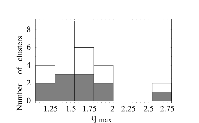
Figure 4.— Distribution of maximum axial ratios. The gray histogram is for cooling-flow systems.

Figure 5.— Maximum axial ratio as a function of the redshift. The solid and dashed lines represent the linear best fit to the data with and without weights, respectively.

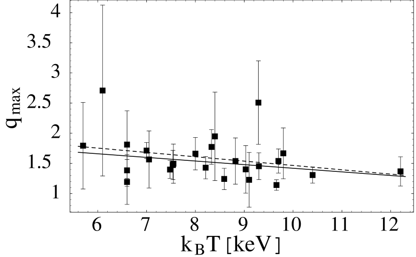
Figure 6.— Maximum axial ratio as a function of temperature. The solid and dashed lines represent the linear best fit to the data with and without weights, respectively.

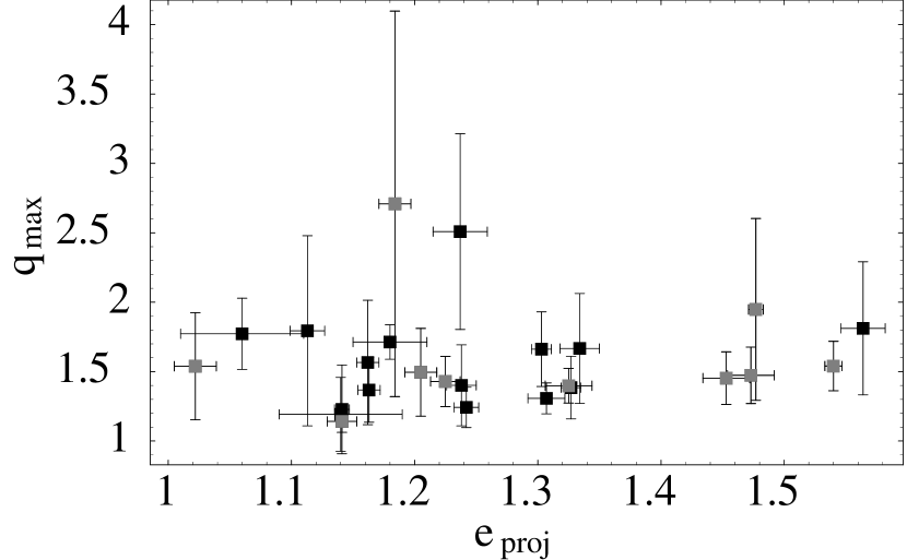
Figure 7.— Cluster maximum axial ratio as function of (projected) ellipticity in the p.o.s. Grey squares denote cooling-flow clusters.

6.4. Ellipticity and Prolateness

Triaxial ellipsoids can be represented in the ellipticity-prolateness plane $(E,P)$ (Thomas et al., 1998; Sulkanen, 1999). The ellipticity is defined as:

$$E=\frac{1}{2}\frac{e_{\rm max}^{2}-e_{\rm min}^{2}}{e_{\rm min}^{2}+e_{\rm med}^{2}+e_{\rm max}^{2}}$$ (16)

and the prolateness as:

$$P=\frac{1}{2}\frac{e_{\rm min}^{2}-2e_{\rm med}^{2}+e_{\rm max}^{2}}{e_{\rm min}^{2}+e_{\rm med}^{2}+e_{\rm max}^{2}}$$ (17)

where the axial ratios satisfy $e_{\rm min}\leq e_{\rm med}\leq e_{\rm max}$. The allowed region in the $(E,P)$ plane is a triangle delimited by the lines on which prolate and oblate clusters fall ($P=-E$ and $P=E$, respectively) and the line connecting their endpoints. Fig. 8 shows the distribution in ellipticity-prolateness for our sample. No cluster in our sample shows extreme values of the ellipticity parameter. As expected from some simulations (Kasun & Evrard, 2004), prolate shapes ($P>0$) may be more likely ($18$ clusters) than oblate ones ($P<0$). Once again, cooling flow clusters (gray boxes) are indistinguishable from the sample as a whole.

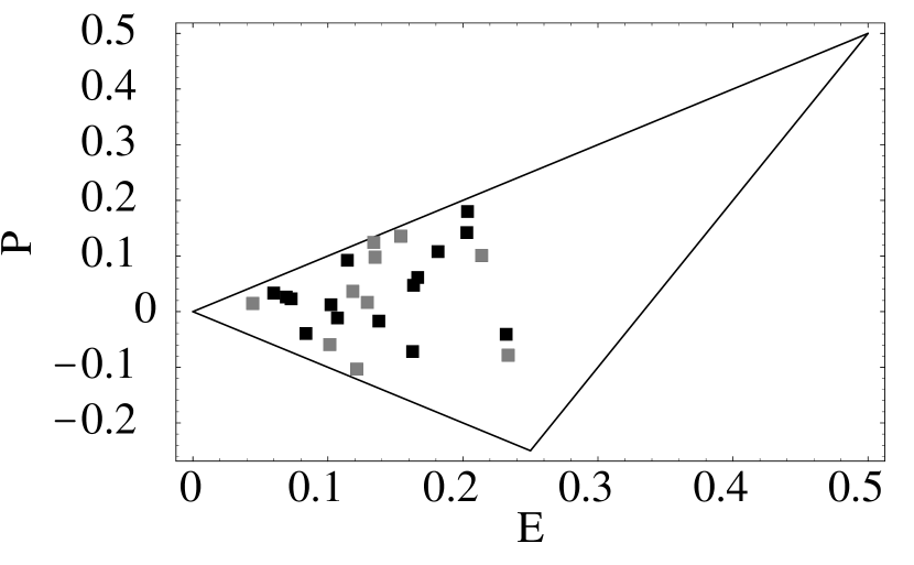
Figure 8.— Distribution in the ellipticity-prolateness plane for our sample. Grey squares highlight cooling-flow clusters.

7. Summary and Discussion

In this paper we have discussed how observations of clusters in the microwave and X-Ray spectral bands can be combined to constrain their intrinsic 3-D shapes, provided that the cosmological model is known. We have applied our method to a combined sample of $25$ clusters of galaxies. In doing so we make the simplifying assumption that the clusters are ellipsoids with one axis parallel to the l.o.s.
Our sample clusters were originally selected on the basis of X-Ray luminosity, with the selection threshold well above the detection limit, in order to avoid selection on the basis of X-Ray surface brightness. Even so, we observe that clusters with extreme axes ratios are still preferentially selected only if the elongation lies along the l.o.s.
The mean value of the axial ratio in low-density cosmological simulations ranges from $1.56$ (Suwa et al., 2003; Kasun & Evrard, 2004) to $1.8$ (Jing & Suto, 2002) and $2.0$ (Thomas et al., 1998). This is consistent with results we present here $\langle q_{\rm max}\rangle=1.59{\pm}0.07$. The spherical hypothesis is generally rejected, with prolate-like shapes being slightly more likely than oblate-like ones. Numerical investigations suggest there should be some tendency for axial ratios to be larger at higher redshift (Jing & Suto, 2002; Suwa et al., 2003; Kasun & Evrard, 2004), though this effect is only marginal: the axial ratio increases only $3\%$ from $z=0$ to $z=0.8$ (Kasun & Evrard, 2004). Our data are not sufficiently precise to test this prediction. A poor correlation is also observed between the maximum axial ratio and the cluster gas temperature. The absence of such a correlation may indicate that high cluster temperatures are not mainly the result of shocks associated with accretion of sub-clusters, since such events would likely produce departures from spherical morphology.
The uncertainties on our results are mainly due to the relatively large errors in the SZE measurements of central temperature decrement, together with the quadratic dependence of the distance estimates on this parameter. More accurate SZE measurements, with better effective angular resolution, are required to extend this analysis to a large sample spanning a greater redshift range.
A relevant number of cosmological tests are today based on the knowledge of the mass of galaxy clusters through X-Ray measurements; these masses are though usually computed assuming a spherical symmetry. It is therefore extremely important to assess the effect that such assumption has on the determination of the total cluster mass. We have estimated that while the effect is negligible when the mass is computed at large distances from the cluster center, the discrepancy between the two mass values becomes much more important as we get closer to the cluster core (i.e. $\approx 25\%$ when the mass is computed within a radius of $100\ {\rm kpc}$). Triaxial cluster shapes may therefore at least partially account for the discrepancies between cluster mass computed with strong lensing and X-Rays data.
Although the presence of a cooling flow is often interpreted as a sign of dynamical relaxation, the properties of the subsample of $10$ cooling flow clusters do not differ from those of the whole sample: cooling flow clusters therefore do not show preferentially spherical morphologies.

Appendix A A. Triaxial Ellipsoids

We consider a cluster electron density distribution described by an ellipsoidal triaxial $\beta$-model. In a $\beta$-model, the electron density of the intra-cluster gas is assumed to be constant on a family of similar, concentric, coaxial ellipsoids. High resolution $N$-body simulations have shown the asphericity of density profiles of dark matter halos and how such profiles can be accurately described by concentric triaxial ellipsoids with aligned axis: ellipsoidal $\beta$-models therefore provide a more detailed description of relatively relaxed simulated halos, respect to the conventional spherically symmetric model (Jing & Suto, 2002).
In a coordinate system relative to the cluster, we then describe the cluster electron density as:

$$n_{e}=n_{e0}\left(1+\frac{\sum_{i=1}^{3}v_{i}^{2}x_{i,\rm int}^{2}}{r_{\rm c}^{2}}\right)^{-3\beta/2}$$ (A1)

where $\left\{x_{i,\rm int}\right\}$, with $i=1,2,3$, define an intrinsic orthogonal coordinate system centered on the cluster’s barycenter and whose coordinates are aligned with its principal axes; $r_{\rm c}$ is the characteristic length scale of the distribution, which in our case is defined as the core radius; along each axis, $v_{i}$ is the inverse of the corresponding core radius in units of $r_{\rm c}$; $n_{e0}$ is the central electron density. The electron density distribution in Eq. (A1) is described by 5 parameters: $n_{e0}$, $\beta$, the axial ratios $e_{1}\equiv v_{1}/v_{3}$ and $e_{2}\equiv v_{2}/v_{3}$, and the core radius $r_{\rm c3}=r_{\rm c}/v_{3}$ along $x_{3,\rm int}$:

$$n_{e}=n_{e0}\left(1+\frac{e_{1}^{2}x_{1,\rm int}^{2}+e_{2}^{2}x_{2,\rm int}^{2}+x_{3,\rm int}^{2}}{r_{\rm c3}^{2}}\right)^{-3\beta/2}$$ (A2)

To write the electron density distribution given by Eq. (A2) in a coordinate system relative to the observer, three additional parameters are needed: the rotation angles -$\theta_{\rm Eu},\varphi_{\rm Eu}$ and $\psi_{\rm Eu}$- of the three principal cluster axes respect to the observer. A rotation through the first two Euler angles is sufficient to align the $x_{3,\rm obs}$-axis of the observer coordinates system $\left\{x_{i,\rm obs}\right\}$ with the l.o.s. of the observer, i.e. the direction connecting the observer to the cluster center. When viewed from an arbitrary direction, quantities constant on similar ellipsoids project themselves on similar ellipses (Stark, 1977). A third rotation -$\psi_{\rm Eu}$- will align $x_{1,\rm obs}$ and $x_{2,\rm obs}$ with the symmetry axes of the ellipses projected on the p.o.s. of the observer (p.o.s.). Eight independent parameters are therefore required to uniquely geometrically characterize the electron density distribution of a triaxial galaxy cluster.
The axial ratio of the major to the minor axes of the observed projected isophotes, $e_{\rm proj}(\geq 1)$, is a function of the shape parameters and of the direction of the l.o.s., defined by the first two Euler angles, $\theta_{\rm Eu}$ and $\phi_{\rm Eu}$. It is given by (Binggeli, 1980):

$$e_{\rm proj}=\sqrt{\frac{j+l+\sqrt{(j-l)^{2}+4k^{2}}}{j+l-\sqrt{(j-l)^{2}+4k^{2}}}},$$ (A3)

where $j,k$ and $l$ are:

$$j = e_{1}^{2}e_{2}^{2}\sin^{2}\theta_{\rm Eu}+e_{1}^{2}\cos^{2}\theta_{\rm Eu}\cos^{2}\varphi_{\rm Eu}+e_{2}^{2}\cos^{2}\theta_{\rm Eu}\sin^{2}\varphi_{\rm Eu}$$ (A4)

$$k = (e_{1}^{2}-e_{2}^{2})\sin\varphi_{\rm Eu}\cos\varphi_{\rm Eu}\cos\theta_{\rm Eu}$$ (A5)

$$l = e_{1}^{2}\sin^{2}\varphi_{\rm Eu}+e_{2}^{2}\cos^{2}\varphi_{\rm Eu}$$ (A6)

The rotation angle between the principal axes of the observed ellipses and the projection onto the sky of the ellipsoid $x_{3,\rm int}$-axis is (Binney, 1985):

$$\psi=\frac{1}{2}\arctan\left[\frac{2k}{j-l}\right].$$ (A7)

The apparent principal axis that lies furthest from the projection onto the sky of the $x_{3,\rm int}$-ellipsoid axis is the apparent major axis if  (Binney, 1985)

$$(j-l)\cos 2\psi+2k\sin 2\psi\leq 0$$ (A8)

or the apparent minor axis otherwise. In what follows, we assume $x_{1,\rm obs}$ to lie along the major axis of the isophotes, so that:

$$\psi_{\rm Eu}=\arctan\left[\frac{2k}{j-l-\sqrt{4k^{2}-(j-l)^{2}}}\right].$$ (A9)

The projected axial ratio $e_{\rm proj}$, the orientation angle of the projected ellipses, the slope $\beta$ and the projection in the p.o.s. of the core radius can be determined fitting observed images to the $\beta$-model; further independent constraints are therefore still required to uniquely determine the gas distribution.
The X-Ray surface brightness and the SZ temperature decrement are given by projection along the l.o.s. of two different powers of the electron density $n_{e}$. Following Stark (1977), we calculate the projection along the l.o.s. of the electron density distribution, given by Eq. (A2), to a generic power $m$ which, in the observer coordinate system, can be written as:

$$\int_{\rm l.o.s.}n_{e}^{m}(x_{1,\rm obs},x_{2,\rm obs},l)dl=n_{e0}^{m}\sqrt{\pi}\frac{\Gamma\left[3m\beta/2-1/2\right]}{\Gamma\left[3m\beta/2\right]}\frac{D_{\rm c}\theta_{\rm c3}}{\sqrt{h}}\left(1+\frac{\theta_{1}^{2}+e_{\rm proj}^{2}\theta_{2}^{2}}{\theta_{c,\rm proj}^{2}}\right)^{(1-3m\beta)/2}$$ (A10)

where $D_{\rm c}$ is the angular diameter distance to the cluster and $\theta_{i}\equiv x_{i,\rm obs}/D_{\rm c}$ is the projected angular position on the p.o.s. of $x_{i,\rm obs}$. $h$ is a function of the cluster shape and orientation:

$$h=e_{1}^{2}\sin^{2}\theta_{\rm Eu}\sin^{2}\varphi_{\rm Eu}+e_{2}^{2}\sin^{2}\theta_{\rm Eu}\cos^{2}\varphi_{\rm Eu}+\cos^{2}\theta_{\rm Eu}$$ (A11)

The observed cluster angular core radius $\theta_{c,\rm proj}$ is the projection on the p.o.s. of the cluster angular intrinsic core radius

$$\theta_{\rm c,proj}\equiv\theta_{\rm c3}\left(\frac{e_{\rm proj}}{e_{1}e_{2}}\right)^{1/2}h^{1/4}$$ (A12)

where $\theta_{\rm c3}\equiv r_{\rm c3}/D_{\rm c}$.

Appendix B B. Inclination Issues

The analysis presented above is based on the main assumption that one cluster principal axis is elongated along the line of sight. Despite this assumption is quite strong, it does not affect significantly the results. To test the effect of inclination on the estimate of the axis ratios, we proceed in the following way. First, we generate a galaxy cluster, characterized by the maximum axis ratio $q_{\mathrm{max}}$ and by a parameter related to the degree of triaxiality, $T\equiv\left(e_{\mathrm{mid}}-e_{\mathrm{min}}\right)/\left(e_{\mathrm{max}}-e_{\mathrm{min}}\right)$; oblate and prolate clusters correspond to $T=0$ and 1, respectively. Since we are only interested in inclination issues, we neglect other measurements errors. Then, we generate a set of 25 viewing angles $\left\{\theta_{\mathrm{Eu}},\varphi_{\mathrm{Eu}}\right\}$. We assume that orientations are completely random, i.e. the angle $\theta_{\mathrm{Eu}}$ is between 0 and $\pi$ and follows the distribution $\sin\theta_{\mathrm{Eu}}/2$, whereas $\varphi_{\mathrm{Eu}}$ follows a uniform distribution between 0 and $2\pi$. For each pair of orientation angles, we compute the projected ellipticity $e_{\mathrm{proj}}$ and the elongation $e_{\mathrm{l.o.s.}}$ and, then, we obtain an estimate of the axial ratios of the cluster in the hypothesis of one principal axis being aligned along the l.o.s. Finally, we calculate mean and standard deviation of the set of axial ratios corresponding to different viewing angles. If the value of such a mean is near that of the simulated cluster, then inclination issues hardly affect our analysis. In Fig. 9, we plot the effect on the estimate of $q_{\mathrm{max}}$ for different values of T in the case of $q_{\mathrm{max}}=1.5$. Error bars equal standard deviations. As we can see, the error is minimum for highly triaxial clusters ($T\sim 0.5$), being $\sim 0.1$. Such an error should be added in quadrature to the value of $\Delta q_{\mathrm{max}}$ estimated in the previous sections, but due to its smallness it does not contribute significantly. The error increases for oblate or prolate clusters, with values $\stackrel{{\scriptstyle<}}{{\sim}}0.4$. In this paper we have been facing with the hypothesis of triaxial clusters, in fact the algorithm illustrated in the previous sections is optimized to describe triaxial spheroids. The capability of ellipsoids of revolution to reproduce the observed data set will be the subject of a forthcoming paper. This considerations are quite general and still holds for very different values of $q_{\mathrm{max}}$. The error due to inclination issue on the estimate of axial ratios can be usually neglected with respect to other uncertainties, in particular in the measurement of the SZ temperature decrement.

Figure 9.— The error in the estimate of the axial ratio, $q_{\mathrm{max}}$, due to inclination issue vs. the triaxiality degree. The horizontal line is fixed to the true value of $q_{\mathrm{max}}$. Points with error bars refer to estimates in the hypothesis of one principal axis oriented along the l.o.s.

Appendix C C. Gravitational Lensing

Clusters of galaxies act as lenses deflecting light rays from background galaxies. In contrast to SZE and X-Ray emission, gravitational lensing does not probe directly the ICM distribution but maps the cluster total mass. The ICM distribution in clusters of galaxies traces the gravitational potential. Since we are considering a triaxial $\beta$-model for the gas distribution, the gravitational potential turns out to be constant on a family of similar, concentric, coaxial ellipsoids. Ellipsoidal potentials are widely used in gravitational lensing analyses to fit multiple image systems (Schneider et al., 1992).
The distribution of the cluster total mass can be inferred from its gas distribution. If the intra-cluster gas is assumed to be isothermal and in hydrostatic equilibrium in the cluster gravitational potential, while non-thermal processes are assumed not to contribute significantly to the gas pressure, the total dynamical mass density reads:

$$\rho_{\rm tot}=-\left(\frac{k_{B}T_{\rm e}}{4\pi G\mu m_{\rm p}}\right)\nabla^{2}\left(\ln n_{\rm e}\right)$$ (C1)

where $G$ is the gravitational constant and $\mu m_{\rm p}$ is the mean particle mass of the gas. If we assume that the electron density of the ICM follows a $\beta$-model distribution given by Eq. (A2), the total gravitating mass density, in the coordinate system relative to the cluster, is given by:

$$\rho_{M}=\frac{3\beta k_{\rm B}T_{\rm e}}{4\pi G\mu m_{\rm p}r_{\rm c3}^{2}}\left(1+\frac{r_{\rm ell}^{2}}{r_{\rm c3}^{2}}\right)^{-1}\left[\sum_{i=1}^{3}e_{i}^{2}-\frac{2}{r_{\rm c3}^{2}}\frac{\sum_{i=1}^{3}\left(e_{i}^{2}x_{i,\rm int}\right)^{2}}{1+r_{\rm ell}^{2}/r_{\rm c3}^{2}}\right]$$ (C2)

where $e_{3}=1$ and $r_{\rm ell}$ is the ellipsoidal radius, $r_{\rm ell}^{2}\equiv\sum_{i=1}^{3}\left(e_{i}x_{i,\rm int}\right)^{2}$. The projected surface mass density can subsequently be written, in the observer reference frame, as:

$$\Sigma=\Sigma_{0}\left(1+\frac{e_{\rm proj}^{2}}{1+e_{\rm proj}^{2}}\frac{\theta_{1}^{2}+\theta_{2}^{2}}{\theta_{\rm c,proj}^{2}}\right)\left(1+\frac{\theta_{1}^{2}+e_{\rm proj}^{2}\theta_{2}^{2}}{\theta_{\rm c,proj}^{2}}\right)^{-3/2}$$ (C3)

where:

$$\Sigma_{0}=\frac{3}{4}\frac{\beta k_{\rm B}T_{\rm e}}{G\mu m_{\rm p}}\frac{\sqrt{e_{1}e_{2}}}{h^{3/4}}\frac{1+e_{\rm proj}^{2}}{\sqrt{e_{\rm proj}}}\frac{1}{\theta_{\rm c,proj}}\frac{1}{D_{\rm c}}$$ (C4)

Although the hypotheses of hydrostatic equilibrium and isothermal gas are very strong, total mass densities obtained under such assumptions can yield accurate estimates even in dynamically active clusters with irregular X-Ray morphologies. Elliptical potentials motivated by X-Ray observations were employed in the irregular cluster AC 114 to provide good fit to multiple image systems (De Filippis et al., 2004).
The lensing effect is determined by the convergence $k$:

$$k=\frac{\Sigma}{\Sigma_{\rm cr}}$$ (C5)

which is the cluster surface mass density in units of the surface critical density $\Sigma_{\rm cr}$:

$$\Sigma_{\rm cr}\equiv\frac{c^{2}}{4\pi G}\frac{D_{\rm s}}{D_{\rm c}D_{\rm cs}}$$ (C6)

where $D_{\rm cs}$ is the angular diameter distance from the lens to the source and $D_{\rm s}$ and $D_{\rm c}$ are the angular diameter distances from the observer to the source and to the lens, respectively. Fitting the observed surface mass density to a multiple image system, it is possible to determine the central value of the convergence:

$$k_{0}(z_{s})=\frac{\Sigma_{0}}{\Sigma_{\rm cr}}$$

which, using Eqs. (C4) and (C6), can be written as:

$$k_{0}(z_{s})=\frac{3\pi\beta k_{\rm B}T_{\rm e}}{c^{2}\mu m_{\rm p}}\frac{\sqrt{e_{1}e_{2}}}{h^{3/4}}\frac{1+e_{\rm proj}^{2}}{\sqrt{e_{\rm proj}}}\frac{1}{\theta_{c,\rm proj}}\frac{D_{\rm cs}}{D_{\rm s}}$$ (C7)

References

- Allen et al. (2004) Allen, S. W., Schmidt, R. W., Ebeling, H., Fabian, A. C., & van Speybroeck, L. 2004, MNRAS, 353, 457
- Binggeli (1980) Binggeli, B. 1980, A&A, 82, 289
- Binney (1985) Binney, J. 1985, MNRAS, 212, 767
- Birkinshaw (1999) Birkinshaw, M. 1999, Phys. Rev., 310, 97
- Cavaliere & Fusco-Femiano (1978) Cavaliere, A., & Fusco-Femiano, R. 1978, åp, 70, 677
- Cooray (1998) Cooray, A. R. 1998, A&A, 339, 623
- D’Agostini (2004) D’Agostini, G. 2004, physics/0403086
- De Filippis et al. (2004) De Filippis, E., Bautz, M. W., Sereno, M., & Garmire, G. P. 2004, ApJ, 611, 164
- Doré et al. (2001) Doré, O., Bouchet, F. R., Mellier, Y., & Teyssier, R. 2001, A&A, 375, 14
- Ebeling et al. (1996) Ebeling, H., Voges, W., Bohringer, H., Edge, A. C., Huchra, J. P., & Briel, U. G. 1996, MNRAS, 281, 799
- Fox & Pen (2002) Fox, D. C., & Pen, U. 2002, ApJ, 574, 38
- Gott et al. (2001) Gott, J. R. I., Vogeley, M. S., Podariu, S., & Ratra, B. 2001, ApJ, 549, 1
- Hughes & Birkinshaw (1998) Hughes, J. P., & Birkinshaw, M. 1998, ApJ, 501, 1
- Inagaki et al. (1995) Inagaki, Y., Suginohara, T., & Suto, Y. 1995, PASJ, 47, 411
- Itoh et al. (1998) Itoh, N., Kohyama, Y., & Nozawa, S. 1998, ApJ, 502, 7
- Jing & Suto (2002) Jing, Y. P., & Suto, Y. 2002, ApJ, 574, 538
- Kasun & Evrard (2004) Kasun, S. F., & Evrard, A. E. 2004, astro-ph/0408056
- Lee & Suto (2004) Lee, J., & Suto, Y. 2004, ApJ, 601, 599
- Lucy (1974) Lucy, L. B. 1974, AJ, 79, 745
- Mason & Myers (2000) Mason, B. S., & Myers, S. T. 2000, ApJ, 540, 614
- Mason et al. (2001) Mason, B. S., Myers, S. T., & Readhead, A. C. S. 2001, ApJ, 555, L11
- Mohr et al. (1995) Mohr, J. J., Evrard, A. E., Fabricant, D. G., & Geller, M. J. 1995, ApJ, 447, 8
- Randall et al. (2002) Randall, S. W., Sarazin, C. L., & Ricker, P. M. 2002, ApJ, 577, 579
- Reblinsky (2000) Reblinsky, K. 2000, A&A, 364, 377
- Reese et al. (2002) Reese, E. D., Carlstrom, J. E., Joy, M., Mohr, J. J., Grego, L., & Holzapfel, W. L. 2002, ApJ, 581, 53
- Richstone et al. (1992) Richstone, D., Loeb, A., & Turner, E. L. 1992, ApJ, 393, 477
- Ryden (1996) Ryden, B. S. 1996, ApJ, 461, 146
- Schneider et al. (1992) Schneider, P., Ehlers, J., & Falco, E. E. 1992, Gravitational Lenses (Gravitational Lenses, XIV, 560 pp. 112 figs.. Springer-Verlag Berlin Heidelberg New York. Also Astronomy and Astrophysics Library)
- Sereno et al. (2001) Sereno, M., Covone, G., Piedipalumbo, E., & de Ritis, R. 2001, MNRAS, 327, 517
- Sereno et al. (2004) Sereno, M., De Filippis, E., & Longo, G. 2004, in preparation
- Sereno et al. (2002) Sereno, M., Piedipalumbo, E., & Sazhin, M. V. 2002, MNRAS, 335, 1061
- Spergel et al. (2003) Spergel, D. N., Verde, L., Peiris, H. V., Komatsu, E., Nolta, M. R., Bennett, C. L., Halpern, M., Hinshaw, G., Jarosik, N., Kogut, A., Limon, M., Meyer, S. S., Page, L., Tucker, G. S., Weiland, J. L., Wollack, E., & Wright, E. L. 2003, ApJS, 148, 175
- Stark (1977) Stark, A. A. 1977, ApJ, 213, 368
- Sulkanen (1999) Sulkanen, M. E. 1999, ApJ, 522, 59
- Sunyaev & Zeldovich (1970) Sunyaev, R. A., & Zeldovich, Y. B. 1970, Comments on Astrophysics, 2, 66
- Suwa et al. (2003) Suwa, T., Habe, A., Yoshikawa, K., & Okamoto, T. 2003, ApJ, 588, 7
- Tegmark et al. (2004) Tegmark, M., Strauss, M. A., Blanton, M. R., Abazajian, K., Dodelson, S., Sandvik, H., Wang, X., Weinberg, D. H., Zehavi, I., Bahcall, N. A., Hoyle, F., Schlegel, D., Scoccimarro, R., Vogeley, M. S., Berlind, A., Budavari, T., Connolly, A., Eisenstein, D. J., Finkbeiner, D., Frieman, J. A., Gunn, J. E., Hui, L., Jain, B., Johnston, D., Kent, S., Lin, H., Nakajima, R., Nichol, R. C., Ostriker, J. P., Pope, A., Scranton, R., Seljak, U., Sheth, R. K., Stebbins, A., Szalay, A. S., Szapudi, I., Xu, Y., Annis, J., Brinkmann, J., Burles, S., Castander, F. J., Csabai, I., Loveday, J., Doi, M., Fukugita, M., Gillespie, B., Hennessy, G., Hogg, D. W., Ivezić, Ž., Knapp, G. R., Lamb, D. Q., Lee, B. C., Lupton, R. H., McKay, T. A., Kunszt, P., Munn, J. A., O’Connell, L., Peoples, J., Pier, J. R., Richmond, M., Rockosi, C., Schneider, D. P., Stoughton, C., Tucker, D. L., vanden Berk, D. E., Yanny, B., & York, D. G. 2004, Phys. Rev. D, 69, 103501
- Thomas et al. (1998) Thomas, P. A., Colberg, J. M., Couchman, H. M. P., Efstathiou, G. P., Frenk, C. S., Jenkins, A. R., Nelson, A. H., Hutchings, R. M., Peacock, J. A., Pearce, F. R., & White, S. D. M. 1998, MNRAS, 296, 1061
- Wang et al. (2000) Wang, L., Caldwell, R. R., Ostriker, J. P., & Steinhardt, P. J. 2000, ApJ, 530, 17
- Zaroubi et al. (2001) Zaroubi, S., Squires, G., de Gasperis, G., Evrard, A. E., Hoffman, Y., & Silk, J. 2001, ApJ, 561, 600
- Zaroubi et al. (1998) Zaroubi, S., Squires, G., Hoffman, Y., & Silk, J. 1998, ApJ, 500, L87