The dust obscuration bias in Damped Lyman $\alpha$ systems

We present a new study of the effects of quasar obscuration on the statistics of Damped Ly $\alpha$ (DLA) systems. We show that the extinction of any Galactic or extragalactic H i region, $A_{\lambda}$, increases linearly with the column density of zinc, with a turning point $\partial A_{\lambda}/\partial(\log N_{\mathrm{Zn}})=1$, above which background sources are suddenly obscured. We derive a relation $A_{\lambda}=A_{\lambda}(N_{\mathrm{H}},Z,z)$ between the extinction of a DLA system and its H i column density, $N_{\mathrm{H}}$, metallicity, $Z$, fraction of iron in dust, $f_{\mathrm{Fe}}(Z)$, and redshift, $z$. From this relation we estimate the fraction of DLA systems missed as a consequence of their own extinction in magnitude-limited surveys. We derive a method for recovering the true frequency distributions of $N_{\mathrm{H}}$ and $Z$ in DLAs, $f_{N_{\mathrm{H}}}$ and $f_{Z}$, using the biased distributions measured in the redshift range where the observations have sufficient statistics ($1.8\leq z\leq 3$). By applying our method we find that the well-known empirical thresholds of DLA column densities, $N_{\mathrm{Zn}}\la 10^{13.1}$ atoms cm^-2 and $N_{H\textsc{i}}\la 10^{22}$ atoms cm^-2, can be successfully explained in terms of the obscuration effect without tuning of the local dust parameters. The obscuration has a modest effect on the distribution of quasar apparent magnitudes, but plays an important role in shaping the statistical distributions of DLAs. The exact estimate of the bias is still limited by the paucity of the data ($\simeq$ 40 zinc measurements at $1.8\leq z\leq 3$). We find that the fraction of DLAs missed as a consequence of obscuration is $\sim$ 30% to 50%, consistent with the results of surveys of radio-selected quasars. By modelling the metallicity distribution with a Schechter function we find that the mean metallicity can be $\sim 5$ to 6 times higher than the value commonly reported for DLAs at $z\sim 2.3$.

1 Introduction

Quasar absorption line systems probe the diffuse gas in the Universe over cosmological scales and at various stages of evolution. Among these absorbers, the Damped Ly$\alpha$ systems (hereafter DLAs) have the highest H i column densities ($N_{H\textsc{i}}\geq 2\times 10^{20}$ atoms cm^-2) and are believed to originate in H i regions of high-redshift galaxies (Wolfe et al. 1986). Also, they have higher metallicities than any other class of quasar absorbers ([M/H] $\approx-1.1$ dex; Pettini et al. 1994) and as such are expected to contain dust. If present, the dust in DLAs will absorb and scatter the radiation of the background quasar, dimming its apparent magnitude (”extinction” effect) and changing the slope of its spectral distribution (”reddening”). In magnitude limited surveys, the extinction may obscure the quasar, leading to an observational selection effect known as obscuration bias (Ostriker & Heisler, 1984; Fall & Pei 1989, 1993).

The bias can lead to misleading conclusions on the nature of the galaxies associated with the DLA systems (herefater DLA galaxies), because the H i regions most enriched by metals and dust would be systematically missed in the surveys. In addition, some properties of the high-redshift Universe that can only be derived from studies of DLAs, would also be affected by the bias. One example is the comoving mass density of neutral gas, $\Omega_{\mathrm{DLA}}$, and its evolution with redshift, which is an indicator of gas consumption due to star formation (Wolfe et al. 1995). Another example is the mean cosmic metallicity inferred from abundance studies of DLAs (Pettini et al. 1997), which is related to the star formation rate in the early Universe (Pei & Fall 1995, hereafter PF95; Pei et al. 1999).

Whether the obscuration effect is important, depends on the actual amount of dust in DLAs. The first evidence of dust, in the form of reddening, was reported by Pei et al. (1991). The complex variability of the quasar continuum makes it impossible to determine the reddening in individual cases. However, from a statistical comparison of quasars with and without foreground DLAs one can search for a systematic change of the continuum slope. In this way, Pei et al. found a systematic difference, suggestive of reddening, using a simplified power-law fit to the continuum distribution.

The detection or reddening motivated detailed studies of quasar obscuration. Fall & Pei (1993; hereafter FP93) presented an analytical method of computing the obscuration from the observed luminosity function of quasars, the typical dust-to-gas ratio of DLAs and the empirical distribution of H i column densities. By modelling the radial distribution of the neutral gas in DLA galaxies, they concluded that a large fraction of quasars may be obscured in optically selected samples. The large uncertainty of the reddening measurements prevented reaching firm conclusions on the dust-to-gas ratios and on the magnitude of the bias.

An alternative approach to measure the amount of the dust in DLAs consists in measuring the differential depletions between refractory and volatile elements (Pettini et al. 1994; Hou et al. 2001; Prochaska & Wolfe 2002; Ledoux et al. 2003; Vladilo 2002, 2004). The depletions can be converted into dust-to-gas ratios, yielding an approximate estimate of the quasar extinction (Vladilo et al. 2001b; Prochaska & Wolfe 2002). This method, as well as the reddening measurements, only give information on the detected DLAs, leaving open the possibility that more dusty H i regions remain undetected.

A more direct probe of the obscuration effect is a comparison of DLA statistics in optically selected and radio selected quasar samples, given that the latter are unaffected by dust extinction. Ellison et al. (2001) compiled a homogeneous sample of radio selected quasars and searched for DLAs towards every target, irrespective of its optical magnitude (CORALS survey). They concluded that dust-induced bias in previous magnitude limited surveys may have led to underestimating the H i mass density, $\Omega_{\mathrm{DLA}}$, and the number density per unit redshift interval, $n(z)$, of DLAs by at most a factor of two at $z\sim 2.3$. In addition, they found tentative evidence that $n(z)$ is greater in fainter quasars, as expected by the obscuration effect. In a follow-up study of CORALS metallicities, Akerman et al. (2005) find $[<\mathrm{Zn/H}>]=-0.88\pm 0.21$. This value is higher than in a control sample, as expected by the obscuration, but only at $1\sigma$ level. In an extension of the CORALS survey at $0.6<z<1.7$ Ellison et al. (2004) find $n(z)=0.16^{+0.08}_{-0.06}$ using MgII absorbers as DLA candidates. This value is consistent with magnitude-limited estimates at the same $z$, but the $1\sigma$ error permits a factor of 2.5 difference in the sense predicted by the obscuration.

The results of the CORALS survey are not yet conclusive since the original sample of Ellison et al. had limited statistics, in particular at the high values of $N({H\textsc{i}})$ where the effect is expected to be more important. This weak evidence of obscuration, together with the non-detection of reddening in a large sample of quasars with and without candidate DLAs, recently reported by Murphy & Liske (2004), are conveying the impression that the obscuration effect is not important.

Yet, indirect evidence for the existence of the bias comes from other studies. The analysis of [Zn/H] versus $\log N({H\textsc{i}})$ by Boissé et al. (1998) showed that none of the DLAs with zinc detection known at the time have a metallicity above the threshold [Zn/H] $+\log N({H\textsc{i}})\simeq 20.5$, corresponding to $N({Zn\textsc{ii}})\simeq 10^{13.1}$ atoms cm^-2. They proposed that this threshold could be attributed to obscuration effect, assuming that metal column density tracks the dust column density.

While this assumption has not been proven by subsequent investigations, the threshold proposed by Boissé et al. has been invoked to reconcile several predictions of galactic evolution models (Prantzos & Boissier 2000; Hou et al. 2001) and cosmological simulations (Cen et al. 2003) with the observed properties of DLAs.

Another potential evidence of the bias is the lack of DLAs with H i column densities $N({H\textsc{i}})\ga 10^{22}$ atoms cm^-2. In this case, the obscuration has been invoked to explain the significant fraction of model galaxy disks predicted to have higher H i column densities (Churches et al. 2004). As an alternative explanation, it has been proposed that hydrogen may undergo a sudden transition from the atomic to the molecular form above a critical column density threshold (Schaye 2001), in which case the absorber would not be detected as a DLA system.

In the present work we address several open questions concerning the existence and importance of the obscuration bias. In Section 2, we perform a careful investigation of all the factors that determine the extinction of a Galactic or extragalactic H i region. In Section 3 we report some indirect evidence of obscuration effects. In Section 4 we present a mathematical formulation aimed at recovering the frequency distributions of H i column densities and metallicities of DLAs from the observed distributions affected by obscuration bias. The first implementation of this method is described in Section 5 and the results are discussed in Section 6.

2 The relation between $N_{\mathrm{Zn}}$ and extinction

We adopt the simplified notation $N_{\mathrm{Zn}}=N({Zn\textsc{ii}})$ and $N_{\mathrm{H}}=N({H\textsc{i}})$, ignoring contributions from ionization states other than the dominant one (see Vladilo et al. 2001a and references therein).

We start by considering a refractory and a volatile element, $\mathrm{E_{r}}$ and $\mathrm{E_{v}}$, with interstellar abundance ratio by number $(\mathrm{E_{r}}/\mathrm{E_{v}})$. The ratio of the total column densities (gas plus dust) of these two elements along an interstellar line of sight will be $N^{\mathrm{tot}}_{\mathrm{r}}/N^{\mathrm{tot}}_{\mathrm{v}}=(\mathrm{E_{r}}/\mathrm{E_{v}}).$ We call $N^{\mathrm{d}}_{\mathrm{E}}$ and $N_{\mathrm{E}}$ the column densities of an element E in the dust and in the gas, respectively. The fraction of atoms of E in dust form will be $f_{\mathrm{E}}\equiv N^{\mathrm{d}}_{\mathrm{E}}/N^{\mathrm{tot}}_{\mathrm{E}}$. From these definitions we have $N^{\mathrm{tot}}_{\mathrm{r}}=N^{\mathrm{d}}_{\mathrm{r}}/f_{\mathrm{r}}$ and $N^{\mathrm{tot}}_{\mathrm{v}}=N_{\mathrm{v}}/(1-f_{\mathrm{v}})$. Combining these relations we have

$$N^{\mathrm{d}}_{\mathrm{r}}=\,{f_{\mathrm{r}}\over(1-f_{\mathrm{v}})}\,\left({{\mathrm{E_{r}}\over\mathrm{E_{v}}}}\right)\,N_{\mathrm{v}}\leavevmode\nobreak\ .$$ (1)

We next consider the relation between $N^{\mathrm{d}}_{\mathrm{r}}$ and the column density of dust grains, $N_{\mathrm{gr}}$, i.e. the number of grains per cm² along the line of sight. For spherical grains of radius $r_{\mathrm{gr}}$ (cm) and internal mass density $\varrho_{\mathrm{gr}}$ (g cm^-3) it is easy to show that

$$N^{\mathrm{d}}_{\mathrm{r}}\,\mathrm{A_{r}}\,m_{\mathrm{H}}={4\over 3}\,\pi\leavevmode\nobreak\ r_{\mathrm{gr}}^{3}\leavevmode\nobreak\ \varrho_{\mathrm{gr}}\leavevmode\nobreak\ N_{\mathrm{gr}}\leavevmode\nobreak\ X^{\mathrm{d}}_{\mathrm{r}}\leavevmode\nobreak\ ,$$ (2)

where $\mathrm{A_{r}}$ is the atomic mass of the refractory element and $X^{\mathrm{d}}_{\mathrm{r}}$ the mass fraction in the dust of the same element.

Finally, we consider the relation between the interstellar extinction in magnitudes at the wavelength $\lambda$, $A_{\lambda}$, and the column density of dust grains. For spherical grains with extinction efficiency factor $Q_{e,\lambda}$ (see Spitzer 1978, Chapter 7) this relation is

$$A_{\lambda}=1.086\leavevmode\nobreak\ N_{\mathrm{gr}}\,\,Q_{e,\lambda}\,\,\pi\,r_{\mathrm{gr}}^{2}\leavevmode\nobreak\ .$$ (3)

By combining Eqs. (1), (2) and (3) we derive

$$A_{\lambda}=a_{\lambda}\leavevmode\nobreak\ N_{\mathrm{v}}\leavevmode\nobreak\ ,$$ (4)

where we define

$$a_{\lambda}=1.817\times 10^{-24}\leavevmode\nobreak\ \mathrm{A_{r}}\leavevmode\nobreak\ g_{\lambda}\leavevmode\nobreak\ {f_{\mathrm{r}}\over(1-f_{\mathrm{v}})}\,\left({{\mathrm{E_{r}}\over\mathrm{E_{v}}}}\right)\leavevmode\nobreak\ ,$$ (5)

and we isolate in the term

$$g_{\lambda}=s\leavevmode\nobreak\ {Q_{e,\lambda}\over r_{\mathrm{gr}}\,\varrho_{\mathrm{gr}}\,X^{\mathrm{d}}_{\mathrm{r}}}\leavevmode\nobreak\$$ (6)

all the properties of the grains (shape, extinction efficiency, size, density, and composition). For spherical grains $s=3/4$.

The factor ${f_{\mathrm{r}}/(1-f_{\mathrm{v}})}$ is approximately constant by definition of volatile and refractory elements. In a medium of constant composition, such as the local ISM, also the abundance $\left({{\mathrm{E_{r}}/\mathrm{E_{v}}}}\right)$ is constant. Therefore, for a given type of dust, the term $a_{\lambda}$ is constant and the expression (4) implies that the interstellar extinction increases linearly with the gas-phase column density of any volatile element measured in the same line of sight.

Differences in the shape, size, density, composition and extinction efficiency of the grains will induce a scatter in the relation. The dependence of $g_{\lambda}$ on the grain size $r_{\mathrm{gr}}$ is linear, while in Eqs. (2) and (3) it was cubic and quadratic. Since the grain size distribution is a key factor in determining the wavelength dependence of the interstellar extinction (see e.g. Draine 2003), the mild dependence of $g_{\lambda}$ on $r_{\mathrm{gr}}$ suggests that the relation between $A_{\lambda}$ and $N_{\mathrm{v}}$ may be similar even in interstellar regions with different types of extinction curves.

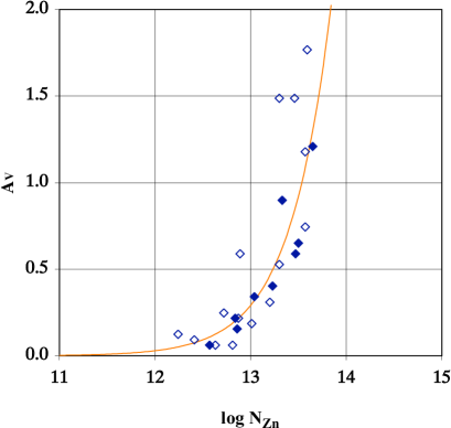
Figure 1: Extinction $A_{V}=R_{V}\,E_{B-V}$ (mag) versus Zn ii column density (atoms cm^-2) in Galactic interstellar lines of sight. Filled diamonds: HST data from Roth & Blades (1995). Empty diamonds: IUE data from Van Steenberg & Shull (1988). Curve: extinction law (7) with $a_{V}=0.29\times 10^{-13}$ mag cm² derived empirically as explained in the text.

By adopting zinc as the volatile element and considering the extinction in the $V$ band ($\lambda_{V}=0.55\mu$m), we obtain from (4) the relation

$$A_{V}\simeq a_{V}\,N_{\mathrm{Zn}}\leavevmode\nobreak\ ,$$ (7)

where the parameter $a_{V}$ (mag cm²) can be determined by comparing measurements of $A_{V}$ and $N_{\mathrm{Zn}}$ in individual lines of sight. In this way it is possible to measure the scatter of $a_{V}$ due to variations of the grain properties.

To estimate $a_{V}$ we gathered the $N_{\mathrm{Zn}}$ measurements obtained from HST (Roth & Blades 1995) and IUE (Van Steenberg & Shull 1988) high-resolution spectra. The IUE data are more numerous, but have lower resolution and signal-to-noise ratio. To reduce the impact of these differences we selected the IUE measurements with total error $<0.3$ dex in $\log N_{\mathrm{Zn}}$. To minimize the contamination by stellar absorptions on top of the IUE Zn ii interstellar lines (Van Steenberg & Shull 1988), we selected only IUE spectra of fast-rotating stars ($V\sin i\geq$ 200 km s^-1). We then scaled the IUE column densities to match the Bergeson & Lawler (1993) Zn ii oscillator strengths adopted in the HST data and in the current research. As far as the extinctions are concerned, we used the $A_{V}$ values given by Guarinos (1991). As a result, we obtained a sample of 11 lines of sight. The mean value of extinction per unit zinc column density that we derive is $<\!\!a_{V}\!\!>\,=0.27(\pm 0.06)\,10^{-13}$ mag cm² and $0.38(\pm 0.20)\,10^{-13}$ mag cm² for the HST and IUE sub-samples (4 and 7 lines of sight, respectively).

In order to enlarge the sample we also considered the color excess $E_{B-V}$, which is more commonly measured than $A_{V}$. The ratio of general-to-selective extinction, $R_{V}={A_{V}/E_{B-V}}$, is approximately constant, with a mean value $<\!\!R_{V}\!\!>\,\simeq 3.1$ in the diffuse ISM of the Milky Way (see e.g. Draine 2003). We used this property to derive a mean value $<\!\!a_{V}\!\!>\,=\,<\!\!R_{V}\!\!>\,<\!\!E_{B-V}/N_{\mathrm{Zn}}\!\!>$ from reddening and zinc column density measurements. The $E_{B-V}$ data were taken from the extinction catalog of Savage et al. (1985). The resulting sample includes 24 lines of sight, shown in Fig. 1. The mean value of the HST sub-sample (9 lines of sight) is $<\!\!a_{V}\!\!>\,=3.1\times 0.089\,(\pm 0.030)\,10^{-13}$ mag cm², and of the IUE sub-sample (15 lines of sight), $3.1\times 0.123\,(\pm 0.071)\,10^{-13}$ mag cm². We did not find significant correlations between $<\!\!E_{B-V}/N_{\mathrm{Zn}}\!\!>$ and the parameters of UV extinction provided by Savage et al. (1985), such as the strength of the emission bump or the steepness of the UV rise. The lack of these correlations gives us a justification for averaging the results obtained from lines of sight with different types of dust.

The results obtained from the $E_{B-V}$ analysis are identical to those obtained from the more limited sample of direct measurements of $A_{V}$. The larger dispersion of the IUE sub-sample is probably due to the lower quality of the data. We adopted the weighted average of the IUE and HST sub-samples, which yields $<\!\!a_{V}\!\!>\,=0.29(\pm 0.07)\,10^{-13}$ mag cm², a value almost identical to that of the HST sub-sample. The relation (7) obtained from this estimate of $a_{V}$ is displayed in Fig. 1 (solid curve). The exponential rise of the extinction is due to the fact that the Zn ii column density is plotted on a logarithmic scale. In this scale the rise of the extinction is mild at low values of $\log N_{\mathrm{Zn}}$, but very fast at high values. The turning point marking the transition between these two regimes can be estimated from the condition $\partial A_{V}/\partial(\log N_{\mathrm{Zn}})=1$. This criterion yields $\log N_{\mathrm{Zn}}=-\log(<\!\!a_{V}\!\!>\,\ln 10)=13.18$. Above this turning point the extinction undergoes a dramatic rise, acting as a barrier against detection of faint background sources. This barrier is remarkably similar to the detection threshold proposed by Boissé et al. (1998). This motivated us to investigate the relation between extinction and metal column density in DLA systems.

2.1 Extinction versus $N_{\mathrm{Zn}}$ in DLA systems

The relations (4), (5) and (6) are valid in the ISM of any galaxy, including DLA systems, which are H i regions of high-redshift galaxies. Applying these relations to a DLA system and to the local ISM, and adopting $\mathrm{E_{v}}$=Zn, $\mathrm{E_{r}}$=Fe and $\lambda=\lambda_{V}$, we obtain

$$A_{V}=a_{V,i}\,{g_{V}\over g_{V,i}}\leavevmode\nobreak\ {(1-f_{\mathrm{Zn},i})\over f_{\mathrm{Fe},i}}\leavevmode\nobreak\ {f_{\mathrm{Fe}}\over(1-f_{\mathrm{Zn}})}\leavevmode\nobreak\ {(\mathrm{Fe/Zn})\leavevmode\nobreak\ \over(\mathrm{Fe/Zn})_{i}}\leavevmode\nobreak\ N_{\mathrm{Zn}}\leavevmode\nobreak\ ,$$ (8)

where the quantities in the local ISM are indicated with the index $i$ and those in the DLA system are not labelled. To take into account the dependence on metallicity, which varies among DLAs, we introduce the metallicity $Z\equiv N^{\mathrm{tot}}_{\mathrm{Zn}}/N_{\mathrm{H}}$, where $N^{\mathrm{tot}}_{\mathrm{Zn}}=N_{\mathrm{Zn}}/(1-f_{\mathrm{Zn}})$ is the total zinc column density (gas plus dust). In this way we obtain the expression

$$A_{V}\simeq A_{\circ}\leavevmode\nobreak\ {G}\leavevmode\nobreak\ f_{\mathrm{Fe}}\leavevmode\nobreak\ {(\mathrm{Fe/Zn})\leavevmode\nobreak\ \,\over(\mathrm{Fe/Zn})_{\sun}}\leavevmode\nobreak\ Z\leavevmode\nobreak\ N_{\mathrm{H}}\leavevmode\nobreak\ ,$$ (9)

where $A_{\circ}\equiv a_{V,i}\,(1-f_{\mathrm{Zn},i})/f_{\mathrm{Fe},i}$ and $G=g_{V}/g_{V,i}$. The constant $A_{\circ}$ is estimated using the value $<\!\!a_{V}\!\!>$ derived in the previous section and the mean values of dust fractions of the local ISM sample ($f_{\mathrm{Zn},i}=0.40$ and $f_{\mathrm{Fe},i}=0.94$). We obtain $A_{\circ}\simeq 1.85\times 10^{-14}$ mag cm², with a relative error of $\simeq\pm 0.15$ dex including the uncertainties of the dust fractions. The DLA extinction will vary according to the Fe/Zn abundance in the medium, the iron depletion and the properties of the grains. We briefly discuss each one of these factors.

Relative abundances of metals do not show strong variations in DLAs, despite significant changes of the absolute metallicity $Z$. The Fe/Zn ratio is very close to solar in metal-poor stars with metallicities typical of DLA systems (Mishenina et al. 2002; Gratton et al. 2003; Nissen et al. 2004; see discussion in Vladilo 2004). Deviations from the solar ratio are measured in stars with extremely low metallicities. Such deviations do not affect the present work in any case, because the dust fraction and the extinction vanish at very low metallicity, as we now discuss. We adopt therefore ${(\mathrm{Fe/Zn})/(\mathrm{Fe/Zn})_{\sun}}=1$.

The depletion of DLAs increases with metallicity (Ledoux et al. 2003). In particular, the dust fraction of iron undergoes a fast rise between between metallicities [Zn/H] $\sim-2$ dex and $-1$ dex, from values close to zero up to values typical of the Milky-Way warm interstellar gas (Vladilo 2004). Here we model this trend with the analytical expression

$$f_{\mathrm{Fe}}(Z)={1\over\pi}\,\left[\arctan\left({\mathrm{[Zn/H]}-\mathrm{[Zn/H]}_{\circ}\over\Delta(\mathrm{[Zn/H]})}\right)+{\pi\over 2}\right]$$

designed to smoothly fit the ISM and DLA data, providing a gradual decrease to zero at very low metallicity.

The dependence on the changes of the grain properties enters through the factor $G$, which scales as $s\,Q_{e,\lambda}\,(r_{\mathrm{gr}}\,\varrho_{\mathrm{gr}}\,X^{d}_{\mathrm{Fe}})^{-1}$ (Eq. 6). This term is mostly determined by the physical conditions of the medium, rather than by its chemical enrichment, with the possible exception of the abundance by mass of iron in the grains, $X^{d}_{\mathrm{Fe}}$. At the very early stages of chemical evolution we may expect variations of $X^{d}_{\mathrm{Fe}}$ as a consequence of non-solar relative abundances of metals. However, these effects do not affect our estimate of the extinction since, at the very low metallicities typical of these early stages ($Z\ll Z_{\sun}$), the factor $f_{\mathrm{Fe}}(Z)$ vanishes in any case, yielding a null extinction.

The variations of $G$ due to changes of the physical conditions can be assessed by sampling different regions in a medium of constant composition, such as the local ISM. The low scatter of $a_{V}$ derived in the previous section indicates that the scatter of $G$ in the local ISM is low, even if the MW sample includes lines of sight with different physical conditions. To explain this qualitatively, we can imagine that variations of the grain size $r_{\mathrm{gr}}$ may compensate variations of the dust density $\varrho_{\mathrm{gr}}$. For instance, in a harsh interstellar environment, volatile elements tend to leave the grains and we may expect an increase of $\varrho_{\mathrm{gr}}$ because carbon, the element potentially most abundant in the grains, is volatile and has low atomic mass. At the same time, we may expect that larger grains will be more easily destroyed in a harsh environment and the mean $r_{\mathrm{gr}}$ will decrease, countering the increase of $\varrho_{\mathrm{gr}}$ in Eq. (6).

These general considerations apply to any type of interstellar environment, suggesting that $G$ may not vary dramatically in DLAs with moderately low abundances ($Z\ga 0.1\,Z_{\sun}$). To test this hypothesis we computed $G$ in the Small Magellanic Cloud (SMC) from the expression

$${G_{\mathrm{SMC}}}\simeq{({A_{V}\over N_{\mathrm{H}}})_{\mathrm{SMC}}\over({A_{V}\over N_{\mathrm{H}}})_{\mathrm{MW}}}\,\left[{Z_{\mathrm{SMC}}\over Z_{\sun}}\,{f_{\mathrm{Fe},\mathrm{SMC}}\over f_{\mathrm{Fe},\mathrm{MW}}}\right]^{-1}\,$$ (10)

obtained by applying Eq. (9) to the SMC with $(\mathrm{Fe/Zn})_{\mathrm{SMC}}=(\mathrm{Fe/Zn})_{\sun}$. Inserting $({A_{V}\over N_{\mathrm{H}}})_{\mathrm{SMC}}=8.7\times 10^{-23}$ mag cm² (Gordon 2003; SMC bar), $({A_{V}\over N_{\mathrm{H}}})_{\mathrm{MW}}=2.1\times 10^{-22}$ mag cm² (Bohlin et al. 1978), $Z_{\mathrm{SMC}}\simeq 0.25\,Z_{\sun}$ (Russel & Dopita 1992), and $f_{\mathrm{Fe},\mathrm{SMC}}(Z_{\mathrm{SMC}})\simeq 0.91\,f_{\mathrm{Fe},\mathrm{MW}}$ from our analytical relation $f_{\mathrm{Fe}}=f_{\mathrm{Fe}}(Z)$, we obtain ${G_{\mathrm{SMC}}}\simeq 0.6$. Considering the uncertainties in this derivation, this result is consistent with the Milky-Way value, suggesting that, indeed, the term $G$ may not vary dramatically in galaxies of moderately low abundances even if the extinction curve is different.

Eq. (9) is valid in the rest frame of the H i region. To derive the extinction in the observer’s frame we need to consider the wavelength dependence of the extinction. In the rest frame of the DLA system the extinction at the wavelength $\lambda^{\prime}$ will be $A_{\lambda^{\prime}}\simeq\xi(\lambda^{\prime})\,\,A_{V}$, where $\xi(\lambda^{\prime})=A(\lambda^{\prime})/A(\lambda_{V})$ is, by definition, the normalized extinction curve. In the observer’s frame the same extinction will appear at $\lambda=\lambda^{\prime}\,(1+z)$, where $z$ is the absorption redshift.

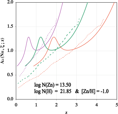
Figure 2: Extinction of a quasar at a fixed wavelength in the observer’s frame, plotted versus the redshift of an intervening DLA system with $N^{\mathrm{tot}}_{\mathrm{Zn}}=10^{13.50}$ cm^-2. Solid and dashed curves represent MW-type and SMC-type extinction curves, respectively (Cardelli et al. 1998; Gordon et al. 2003). Curves left to right: photometric bands $u^{\prime}$, $g^{\prime}$, and $r^{\prime}$, respectively.

In conclusion, the observer’s frame extinction of a quasar at wavelength $\lambda$ due to an intervening DLA system at redshift $z$ is

$$A_{\lambda}(N_{\mathrm{H}},Z;z)\simeq A_{\circ}\leavevmode\nobreak\ G\leavevmode\nobreak\ \,\xi\!\left(\!{\lambda\over 1\!+\!z}\!\right)\leavevmode\nobreak\ f_{\mathrm{Fe}}(Z)\leavevmode\nobreak\ \,N_{\mathrm{H}}\leavevmode\nobreak\ Z\leavevmode\nobreak\ ,$$ (11)

with $A_{\circ}\simeq 1.85\times 10^{-14}$ mag cm², and $G=1$ and $0.6$ for Galactic-type and SMC-type dust, respectively. For each type of dust we adopt the corresponding extinction curve representative of the Milky Way and of the SMC.

Since $\xi(\lambda^{\prime})>1$ for $\lambda^{\prime}<\lambda_{V}$, the net effect of the cosmological redshift is an amplification of the rest-frame extinction at $\lambda<\lambda_{V}\leavevmode\nobreak\ (1+z)$. At $z\ga 2$ this amplification compensates for the reduction of $f_{\mathrm{Fe}}(Z)$ in systems of moderately low metallicity and for the mild reduction of $G$ in SMC-type dust. Only at very low metallicity the extinction becomes negligible since $f_{\mathrm{Fe}}(Z)$ tends to vanish. Overall, the extinction per unit column density of zinc atoms predicted for most DLAs is similar, or even larger, than that typical of the Milky-Way ISM.

Examples of quasar extinction estimated with Eq. (11) are plotted in Fig. 2 as a function of $z$, keeping fixed the other terms. This type of representation puts in evidence the amplification of the extinction with increasing redshift. Each curve was computed at a constant $\lambda$ equal to the effective wavelength of the SLOAN Digital Sky Survey (SDSS) photometric bands $u^{\prime}$, $g^{\prime}$ and $r^{\prime}$ (Fukugita et al. 1996). We adopted the extinction law by Cardelli et al. (1998; hereafter CCM law) with $R_{V}=3.1$ for the Milky-Way extinction curve and the mean SMC bar data by Gordon et al. (2003) for the SMC curve. The term $f_{\mathrm{Fe}}(Z)$ was estimated at [Zn/H] $=\log(Z/Z_{\sun})=-1$ dex. The total zinc column density was fixed at $N^{\mathrm{tot}}_{\mathrm{Zn}}=N_{\mathrm{H}}\,Z=10^{13.50}$ atoms cm^-2, roughly two times the zinc column density threshold proposed by Boissé et al. (1998). For the redshift interval typical of most DLAs ($z\approx 2/3$) the predicted extinction is $\raisebox{-5.0pt}{$\;\stackrel{{\scriptstyle\textstyle>}}{{\sim}}\;$}1$ mag, a value sufficient to obscure quasars in spectroscopic surveys.

Figure 3: Diamonds: column densities $N_{\mathrm{H}}$ versus $N_{\mathrm{Zn}}$ in DLAs. Horizontal lines: DLA definition threshold (bottom) and empirical upper boundary (top) of $N_{\mathrm{H}}$. Vertical lines: detection limit (left) and obscuration threshold (right) of $N_{\mathrm{Zn}}$. Dashed lines: lines of constant metallicity. Circles: Milky Way data of Fig. 1. Star: GRB-DLA from Savaglio et al. (2003).

3 Evidence for extinction from DLA data

To search for some extinction effect related to the zinc column density we collected from the literature all DLAs with available $N_{\mathrm{Zn}}$ measurements. The resulting sample, shown in Fig. 3, includes 41 measurements, most of which derived from Hires/Keck and UVES/VLT spectra. References to these data can be found in Vladilo (2004; table 1), with the exception of 4 systems (without Fe ii lines) published by Pettini et al. (1994, 1997) and Boissé et al. (1998).

The updated sample includes more than twice the measurements of the one discussed by Boissé et al. (1998) but, in spite of this increase, column densities above the original threshold (line AB in the figure) are not found. The lack of DLAs with $N_{\mathrm{Zn}}>10^{13.1}$ atoms cm^-2 is surprising, since Milky Way lines of sight with Zn ii measurements do show values above this limit in a significant fraction of cases (Fig. 3). Studies of gamma-ray bursts (GRBs) observed inmediately after the explosion demonstrate that zinc column densities above the threshold exist and can be detected in extragalactic absorbers (Savaglio et al. 2003; the only case with measured $N_{\mathrm{H}}$ is indicated with a star in Fig. 3).

These results confirm that some selection effect is preventing the detection of values of $N_{\mathrm{Zn}}$ above the threshold when the background source is faint. The remarkable similarity between the DLA cutoff at $N_{\mathrm{Zn}}=10^{13.1}$ atoms cm^-2 and the ISM turning point at $N_{\mathrm{Zn}}\simeq 10^{13.2}$ suggests that the rapid rise of the extinction above the turning point can be responsible for the cutoff. This is consistent with the conclusion of the previous section that the extinction per unit zinc column density of many DLAs is similar to that of the local ISM.

Figure 4: Normalized frequency distribution of quasar apparent magnitudes for the sub-sample of DLAs with $\log N_{\mathrm{Zn}}>12.53$ (shaded histogram) and $\log N_{\mathrm{Zn}}\leq 12.53$ (light histogram).

If the extinction increases with $N_{\mathrm{Zn}}$, we expect to find evidence of this effect also below the threshold, in the range $\log N_{\mathrm{Zn}}\la 13.1$ where we do detect DLAs. To search for this evidence we analysed the frequency distribution of quasar apparent magnitudes of the zinc sample. We used the $V$ magnitude, which is measured in most cases. In 4 quasars without $V$ measurements we adopted the magnitude of nearby optical bands. In practice, we compared the behaviour of the two sub-samples with $\log N_{\mathrm{Zn}}$ below and above the median value, $(\log N_{\mathrm{Zn}})_{\mathrm{median}}=12.53$. The differences between the two distributions, shown in Fig. 4, are consistent with a rise of the quasar extinction with increasing $N_{\mathrm{Zn}}$. The analysis of the three bins with more statistics indicates that the maximum of the sub-sample with high $N_{\mathrm{Zn}}$ (shaded histogram) is shifted by $\approx 1$ bin relative to the maximum of the other sub-sample (light histogram). A Kolmogorov-Smirnov test shows that there is only a 9.7% level of probability that the two distributions are drawn from the same parent population. The shift to fainter magnitudes suggests that even at $\log N_{\mathrm{Zn}}\raisebox{-5.0pt}{$\;\stackrel{{\scriptstyle\textstyle<}}{{\sim}}\;$}13.1$ dust extinction is already present, affecting more the high-$N_{\mathrm{Zn}}$ sub-sample. The magnitude of this effect can only be explained by invoking a redshift amplification of the extinction, as predicted by relation (11), since the extinction expected at rest-frame is only $\simeq 0.35$ mag at $\log N_{\mathrm{Zn}}=13.1$ (Fig. 1).

4 Mathematical formulation of the bias

In Eq. (11) the variation of the depletion in DLAs is accounted for by the term $f_{\mathrm{Fe}}(Z)$, which is determined by the metallicity. The term $G$ is approximately constant, at least in galaxies with metallicity similar to those of the SMC and Milky Way. Possible variations of $G$ in galaxies of very low metallicity do not affect the prediction of the extinction since, in any case, $f_{\mathrm{Fe}}(Z)$ vanishes when $Z\ll Z_{\sun}$. For these reasons, relation (11) allows us to estimate the extinction of a DLA system using, in practice, only its H i column density and metallicity. We use this property to derive a mathematical formulation of the obscuration bias based on the study of the distribution functions of $N_{\mathrm{H}}$ and $Z$ in DLA systems. In practice, we determine the fraction of DLAs that are missed as a consequence of their own extinction. We then assume that multiple DLA absorbers in a given line of sight play a negligible role in the estimate of the obscuration bias. In this way, as we show in the Appendix, we derive a mathematical formulation of the bias which only makes use of observable statistical distributions of DLAs and quasars. To quantify the obscuration effect we need a good statistics of the observed distributions and this requirement limits the redshift range where our method can be presently applied, since the bulk of DLAs data are currently concentrated in $1.8\raisebox{-5.0pt}{$\;\stackrel{{\scriptstyle\textstyle<}}{{\sim}}\;$}z\raisebox{-5.0pt}{$\;\stackrel{{\scriptstyle\textstyle<}}{{\sim}}\;$}3.0$.

An advantage of our formulation is that it does not require a knowledge of the intrinsic luminosity function of quasars or the geometrical distribution of the neutral gas in DLA galaxies. We refer to FP93 for a mathematical treatment of the effect of quasar obscuration which describes the relation with the quasar luminosity function and the geometrical distribution of the gas in the intervening galaxies.

4.1 True and biased distributions

We consider the DLAs in the redshift interval $(z_{\mathrm{min}},z_{\mathrm{max}})$ that are detectable in a survey with limiting magnitude $m_{\ell}$. We call $f_{N_{\mathrm{H}}}dN_{\mathrm{H}}$ the number of such DLAs with column densities between $N_{\mathrm{H}}$ and $N_{\mathrm{H}}+dN_{\mathrm{H}}$ and $f_{Z}\,dZ$ the number of those with metallicity between $Z$ and $Z+d\,Z$. The distributions $f_{N_{\mathrm{H}}}$ and $f_{Z}$ are defined in absence of obscuration bias and we call them the ”true” distributions. When we consider the effect of the extinction generated by these DLAs, the number of detectable systems will be $f^{\mathrm{b}}_{N_{\mathrm{H}}}dN_{\mathrm{H}}$ and $f^{\mathrm{b}}_{Z}\,dZ$. We call $f^{\mathrm{b}}_{N_{\mathrm{H}}}$ and $f^{\mathrm{b}}_{Z}$ the ”biased” distributions. In the Appendix we derive the following relations between true and biased distributions [see Eqs. (34) and (35)],

$$f^{\mathrm{b}}_{N_{\mathrm{H}}}\simeq{\int_{0}^{\infty}\mathcal{B}_{m_{\ell}}(N_{\mathrm{H}},Z)\,f_{Z}\,d\,Z\over\int_{0}^{\infty}f_{Z}\,d\,Z}\leavevmode\nobreak\ f_{N_{\mathrm{H}}}\leavevmode\nobreak\ \leavevmode\nobreak\$$ (12)

and

$$f^{\mathrm{b}}_{Z}\simeq{\int_{N_{\mathrm{DLA}}}^{\infty}\mathcal{B}_{m_{\ell}}(N_{\mathrm{H}},Z)\,f_{N_{\mathrm{H}}}\,d\,N_{\mathrm{H}}\over\int_{N_{\mathrm{DLA}}}^{\infty}f_{N_{\mathrm{H}}}\,d\,N_{\mathrm{H}}}\leavevmode\nobreak\ f_{Z}\leavevmode\nobreak\ \leavevmode\nobreak\ .$$ (13)

For simplicity we omit the dependence of the equations on $z_{\mathrm{min}}$ and $z_{\mathrm{max}}$. We assume that the statistical distributions of interest smoothly vary inside the redshift interval, so that we can approximate them with their value at mean redshift $\overline{z}=(z_{\mathrm{max}}-z_{\mathrm{min}})/2$, where $\overline{z}$ is close to the peak of the observed distribution.

The ”bias function” $\mathcal{B}_{m_{\ell}}(N_{\mathrm{H}},Z)\equiv B_{m_{\ell}}(N_{\mathrm{H}},Z,\overline{z})$ that transforms the true distributions into the biased ones is given by the relation [see Eq. (27)]

$$B_{m_{\ell}}(N_{\mathrm{H}},Z,z)\equiv{\int_{\circ}^{m_{\ell}-A_{\lambda}(N_{\mathrm{H}},Z,z)}\,n(m;z)\,dm\,\over\int_{\circ}^{m_{\ell}}\,n(m;z)\,dm\,,}$$ (14)

where $A_{\lambda}(N_{\mathrm{H}},Z,z)$ is the DLA extinction and $n(m;z)$ the quasar magnitude distribution.

In the next section we show how to estimate $n(m;z)$, while in Section 4.3 we present a procedure for deriving the true distributions from Eqs. (12) and (13), starting from the observed distributions.

In deriving these equations we made the assumption that the distributions of $N_{\mathrm{H}}$ and $Z$ are statistically independent. We discuss this assumption in Section 4.4.

4.1.1 The quasar magnitude distribution

We call $n(m;z)\,dm$ the number of quasars with apparent magnitude $m\in(m,m+dm)$ observable beyond redshift $z$ all over the sky. This number is defined in absence of quasar obscuration and we call $n(m;z)\,dm$ the ”true” distribution. Our goal is to infer the true distribution from the observed one, which must equal the distribution biased by the obscuration effect, $n^{\mathrm{b}}(m;z)$. The relation between true and biased distribution is discussed in the Appendix (Section A.2), where we derive the equations Eq. (41), i.e.

$$n^{\mathrm{b}}(m;z)\simeq\left[1-\overline{\mathcal{F}}_{1}\right]\,n(m;z)+\,\overline{\mathcal{F}}_{1}\,n^{\mathrm{b}}_{1}(m;z)\leavevmode\nobreak\ ,$$ (15)

and Eq. (42), i.e.

$$n^{\mathrm{b}}_{1}(m;z)=K\int_{-\infty}^{\infty}n(m^{\prime};z)\leavevmode\nobreak\ f_{A_{\lambda}}\!(m-m^{\prime};\overline{z}_{e})\leavevmode\nobreak\ dm^{\prime}\leavevmode\nobreak\ .$$ (16)

In these relations $\overline{\mathcal{F}}_{1}$ is the fraction of quasars with one foreground DLA, $n^{\mathrm{b}}_{1}(m;z)$ the magnitude distribution of quasars with one foreground DLA, $K$ is a normalization factor and $f_{A_{\lambda}}(A_{\lambda};\overline{z}_{e})$ the frequency distribution of the extinctions of the DLAs in the redshift range $z\in(0,\overline{z}_{e})$ ($\overline{z}_{e}$ is the mean redshift of the quasars in the survey). In Section 4.3, we show how to use Eqs. (15) and (16) to infer $n(m;z)$ (see also Appendix A.2).

4.2 Obscuration fraction

We define the obscuration fraction using the mathematical relations between the true and biased distributions. We call total obscuration fraction the quantity

$$\Phi_{m_{\ell}}=1-{\int^{\infty}_{N_{\mathrm{DLA}}}f^{\mathrm{b}}_{N_{\mathrm{H}}}\,dN_{\mathrm{H}}\over\int^{\infty}_{N_{\mathrm{DLA}}}f_{N_{\mathrm{H}}}\,dN_{\mathrm{H}}}\leavevmode\nobreak\ .$$ (17)

The total obscuration fraction represents the number ratio of DLAs missed due to quasar obscuration in a survey with limiting magnitude $m_{\ell}$. The dependence on the limiting magnitude enters in $f^{\mathrm{b}}_{N_{\mathrm{H}}}$ through Eqs. (27) and (34). The total obscuration fraction can also be derived using the true and biased distributions of metallicity.

We call obscuration fraction, $\phi_{m_{\ell}}$, the fraction by number of systems obscured at a particular value of column density or metallicity. For instance, the fraction of systems obscured at a specific value of $N_{\mathrm{H}}$ is

$$\phi_{m_{\ell}}(N_{\mathrm{H}})=1-{f^{\mathrm{b}}_{N_{\mathrm{H}}}\over f_{N_{\mathrm{H}}}}\leavevmode\nobreak\ \leavevmode\nobreak\ .$$ (18)

Similar expressions can be derived to define the obscuration fractions $\phi_{m_{\ell}}(Z)$ and $\phi_{\ell}(N^{\mathrm{t}}_{\mathrm{Zn}})$, i.e. the fraction of systems missed at a particular value of $Z$ and $N^{\mathrm{t}}_{\mathrm{Zn}}$.

4.3 Solution of the equations

The true functions $f_{N_{\mathrm{H}}}$ and $f_{Z}$ are the unknown quantities in Eqs. (12) and (13). The procedure that we follow to solve these equations consists in (i) adopting trial functions $f_{N_{\mathrm{H}}}$ and $f_{Z}$, (ii) estimating $n_{m}\equiv n(m;\overline{z})$, (iii) computing $f^{\mathrm{b}}_{N_{\mathrm{H}}}$ and $f^{\mathrm{b}}_{Z}$ from the equations and (iv) comparing these biased distributions with the observed ones. These steps are repeated by changing the trial functions until the predicted biased functions match the observed ones. We briefly describe each step of this procedure.

In the first step, we adopt analytical functions in parametrical form as the trial functions $f_{N_{\mathrm{H}}}$ and $f_{Z}$. Once we choose the shape, the problem of determining the true functions $f_{N_{\mathrm{H}}}$ and $f_{Z}$ is equivalent to that of determining the values of their parameters.

In the second step we use the trial functions $f_{N_{\mathrm{H}}}$ and $f_{Z}$ to derive the distribution of extinctions from Eq. (11). We use this extinction distribution in Eq. (16). We then iterate Eqs. (15) and (16), starting with a trial function $n(m;z)$, until we find a $n(m;z)$ that yields a perfect agreement between $n^{\mathrm{b}}(m;z)$ and the distribution $n^{\mathrm{obs}}(m;z)$ measured from the surveys.

In the third step we use $n(m;\overline{z})$ to derive $\mathcal{B}_{m_{\ell}}(N_{\mathrm{H}},Z)$ from Eq. (14) and, finally, the biased distributions $f^{\mathrm{b}}_{N_{\mathrm{H}}}$ and $f^{\mathrm{b}}_{Z}$ from Eqs. (12) and (13).

In the last step we compute the $\chi^{2}$ deviation between the predicted distributions $f^{\mathrm{b}}_{N_{\mathrm{H}}}$ and $f^{\mathrm{b}}_{Z}$ and the corresponding observed distributions.

By iterating the steps we determine the parameters of $f_{N_{\mathrm{H}}}$ and $f_{Z}$ which allow $f^{\mathrm{b}}_{N_{\mathrm{H}}}$ and $f^{\mathrm{b}}_{Z}$ to best fit the empirical distributions. The search is done via $\chi^{2}$ minimization. Since we are not guaranteed a priori of the unicity of the solution, we carefully investigate the variation of $\chi^{2}$ in the parameter space to make sure the minimum is unique.

4.4 Are $N_{\mathrm{H}}$ and $Z$ statistically independent ?

The mathematical formulation presented above relies on the assumption that $N_{\mathrm{H}}$ and $Z$ are statistically independent of each other in the true population of DLAs. The local ISM offers an example in support of this independence, since a broad range of H i column densities, including the high values typical of DLAs, are found at constant metallicity, $Z\simeq Z_{\sun}$. Similarly, a DLA system of given metallicity $Z\simeq Z_{\circ}$ will display a distribution of H i column densities, if sampled along random lines of sight. This distribution will reflect the mass spectrum of interstellar clouds, which is likely to be determined by some physical mechanism, such as interstellar turbulence (see discussion in Khersonsky & Turnshek 1996 and refs. therein), rather than by the metallicity. In this sense, it is reasonable to assume that $f_{N_{\mathrm{H}}}$ and $f_{Z}$ are independent distributions.

Independent support of these arguments comes from the hydrodynamic simulations of DLAs evolving in $\Lambda$CDM cosmology (Cen et al. 2003), which indicate that metallicity and hydrogen column density are almost completely uncorrelated. Similar results are found from the cosmological SPH simulations performed by Nagamine et al. (2004).

Notwithstanding, a trend is expected because the metallicity correlates with the star formation rate, which in turn increases with the gas density in the host galaxy. Therefore, lines of sight with high $N_{\mathrm{H}}$ may have a tendency to be associated with higher metallicities. A weak evidence for this trend was found by Cen et al. (2003), but the effect is particularly small at redshift $z\simeq 2-3$. If the metallicity is correlated with $N_{\mathrm{H}}$, the effect of the obscuration is more important than in the ideal case considered above. In this case the application of our mathematical formulation gives a conservative estimate of the bias.

4.5 Gravitational magnification

Competing with the obscuration effect, is the possible gravitational magnification of the background quasar by the absorber itself. Many studies over the years have attempted to estimate the magnitude of this phenomenon for both DLAs (Smette et al. 1997, Le Brun et al. 2000) and metal absorption lines (Vanden Berk et al. 1996, Ménard & Péroux 2003). The results show that for the DLAs selected at optical wavelengths, gravitational effects are small. In the present application of our method, based on DLAs selected at optical wavelength, we therefore neglect the magnification effect.

5 Implementation of the procedure

We describe the statistical distribution functions adopted here as a first example of implementation of the procedure. For the intrinsic distributions we only need to adopt a functional dependence (i.e. a shape), leaving to the procedure the task of determining the parameter values.

5.1 The empirical distributions

We consider the sub-sample of DLA systems with available measurements of Zn ii column densities, for which it is possible to derive metallicities corrected for depletion effects (Vladilo 2004). The differences between the corrected metallicities and the [Zn/H] values taken at face value are small, with a mean value of $+0.12$ dex. Given the size of the zinc sub-sample ($\sim 40$ systems; see list of references in Table 1 of Vladilo 2004) we can estimate the frequency distribution of metallicities with a Poisson statistical error $\la 10\%$ in only a few bins. To make the best use of the available data we selected the systems in the redshift range $1.8\leq z\leq 3$, where most of the $N_{\mathrm{Zn}}$ measurements have been obtained so far. The mean redshift of the sample (28 systems) is $z\simeq 2.3$. To derive the empirical distribution of $N_{\mathrm{H}}$ we used the surveys by Storrie-Lombardi & Wolfe (2000) and Péroux et al. (2003), which have more statistics than the zinc sub-sample. Selecting the DLAs in the range $1.8\leq z\leq 3$ we obtained a sample of $59$ systems.

Then $\log N({H\textsc{i}})$ and [Zn/H]=$\log(Z/Z_{\sun})$, we transformed the derived distributions in linear space, $N({H\textsc{i}})$ and $Z$, for later comparison with the distributions $f_{\mathrm{H}}$ and $f_{Z}$. In computing the biased distributions with our procedure, we took into account the fact that the typical limiting magnitude of the $N_{\mathrm{H}}$ surveys ($m_{\ell}\sim 19.5$) is somewhat larger than that of the metallicity surveys ($m_{\ell}\sim 19$), owing to the different requirements in spectral resolution. In fact, Eqs. (34) and (35) can be solved independently of each other, inserting in each case the appropriate value of $m_{\ell}$.

5.1.1 The frequency distribution of quasar magnitudes

To derive the empirical distribution of quasar magnitudes we used the data of the Sloan Digital Sky Survey (SDSS) (Schneider et al. 2003). The distribution was determined for two photometric bands well representative of the visual part of the spectrum, namely the $g^{\prime}$ and $r^{\prime}$ bands, with effective wavelengths $\lambda=0.48\mu$m and $0.62\mu$m, respectively (Fukugita et al. 1996). In each band we binned the data at steps of 0.5 mag, counting all the quasars located beyond the typical absorption redshift of our sample (in practice, we adopted $2\leq z_{e}\leq 5$). An example of empirical distribution computed for the $g^{\prime}$ band is shown in Fig. 5 (diamonds with error bars). After binning the data, we performed a polynomial fit to the observed $\log n$ - $\log m$ distribution, up to the magnitude $21.5$, for which the statistics and the completeness of the SDSS sample are still good. This fit was adopted as a smooth model of the observed distribution in the magnitude range $17\leq m\leq 21.5$. An example of fit is shown in Fig. 5 (solid line). The limit $m\sim 21.5$ is sufficient for studying the effects of quasar obscuration on the statistics on DLAs since the typical limiting magnitude of DLA surveys is currently $m_{\ell}\raisebox{-5.0pt}{$\;\stackrel{{\scriptstyle\textstyle<}}{{\sim}}\;$}21$.

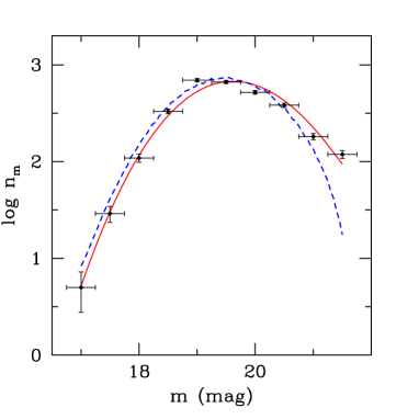
Figure 5: Diamonds: distribution of the SDSS $g^{\prime}$ apparent magnitudes for quasars in the interval $2\leq z_{e}\leq 5$. Smooth lines: example of a pair of model distributions in which the ”true” model (dashed line) is determined from the biased model that fits the observations (solid line), once the distribution of DLA extinctions and $\overline{\mathcal{F}}_{1}$ are specified (see Section 4.1.1).

Table 1: Results.

Ext.curve	Band	$\beta$	$\alpha$	$\log({Z_{\ast}\over Z_{\sun}})$	$\Phi_{22}(m_{\ell})^{a}$	$\Phi_{23}(m_{\ell})^{b}$	$\log({<Z>\over Z_{\sun}})$	$\Omega_{22}^{a}$	$\Omega_{23}^{b}$
					$19.0/19.5$	$19.0/19.5$		$(10^{-3})$	$(10^{-3})$
MW	$r^{\prime}$	1.56	$-0.44$	$-0.13$	$0.41/0.34$	$0.44/0.38$	$-0.37$	$2.3$	$\leavevmode\nobreak\ 7.1$
MW	$g^{\prime}$	1.51	$-0.40$	$-0.10$	$0.48/0.42$	$0.51/0.46$	$-0.31$	$2.8$	$\leavevmode\nobreak\ 9.5$
SMC	$r^{\prime}$	1.61	$-0.46$	$-0.19$	$0.33/0.27$	$0.37/0.30$	$-0.44$	$1.9$	$\leavevmode\nobreak\ 5.5$
SMC	$g^{\prime}$	1.48	$-0.38$	$-0.07$	$0.52/0.46$	$0.56/0.51$	$-0.27$	$3.1$	$11.3$

^a Upper limit of integration in Eq. (17) or (21) truncated at $\log N_{H\textsc{i}}=22$.
^b Upper limit of integration in Eq. (17) or (21) truncated at $\log N_{H\textsc{i}}=23$.

5.2 The shape of the true $N_{\mathrm{H}}$ distribution

One way to approximate the true shape of $f_{N_{\mathrm{H}}}$ is to assume a geometrical distribution of the gas in DLA galaxies. For planar disks with radial exponential profiles $N_{\bot}(r)=N_{\bot 0}\exp(-\alpha\,r)$, the expected frequency distribution is $f_{N_{\mathrm{H}}}\propto N_{\mathrm{H}}^{-1}\leavevmode\nobreak\ \ln N_{\mathrm{H}}$ for $N_{\mathrm{H}}\ll N_{\bot 0}$ and $f_{N_{\mathrm{H}}}\propto N_{\mathrm{H}}^{-3}$ for $N_{\mathrm{H}}\gg N_{\bot 0}$ (FP93). For central column densities $N_{\bot 0}\ga 3\times 10^{21}$ cm^-2 or much larger, as inferred by FP93, this gives $f_{N_{\mathrm{H}}}\propto N_{\mathrm{H}}^{-1}\leavevmode\nobreak\ \ln N_{\mathrm{H}}$ for most of the column-density range typical of DLAs.

A realistic approximation of $f_{N_{\mathrm{H}}}$ should also take into account the fact that, in a given galaxy, the interstellar clouds show a spectrum of masses, $m_{c}$, and sizes, $r_{c}$, which is not accounted for by a smooth radial profile. A large number of studies indicate that the mass spectrum of Milky-Way interstellar clouds follows a power law $f(m_{c})\sim m_{c}^{\gamma}$, with $\gamma=-1.5\pm 0.2$ over a 6 orders of magnitude range of masses (Scalo & Lazarian 1996 and refs. therein). From this mass spectrum, together with a relation between the internal density of the cloud, $n$, and the cloud size we can infer a column-density distribution. Adopting $n\sim r_{c}^{p}$ with $-1.2<p\leq 0$ (Scalo & Lazarian 1996 and refs. therein) we find that the column-density distribution should follow a power law $f_{N_{\mathrm{H}}}\sim N_{\mathrm{H}}^{-\beta}$ with $\beta\geq 2.5$. If this column-density spectrum applies to DLAs, we would expect a decline of column densities faster than that predicted by the exponential profile model.

Both the exponential profile model and the cloud mass-spectrum hypothesis suggest that the true distribution may be approximated with a power law. The hydrodynamic computations of DLAs by Cen et al. (2003) yield a simulated true distribution of $N_{\mathrm{H}}$ consistent with this conclusion.

In light of these considerations, we adopt the simple law $f_{N_{\mathrm{H}}}\sim N_{\mathrm{H}}^{-\beta}$ for the true distribution, with the parameter $\beta$ to be determined by the method itself. If this is a good approximation, the resulting biased distribution $f^{\mathrm{b}}_{N_{\mathrm{H}}}$ must reproduce the observed fast decline of the number of DLAs with column density, which is commonly fitted by a Schechter-type function

$$f_{N_{\mathrm{H}}}\propto{\left(N_{\mathrm{H}}\over N_{\ast}\right)}^{-\beta}\,e^{-\left(N_{\mathrm{H}}\over N_{\ast}\right)},\leavevmode\nobreak\$$ (19)

characterized by a fast decline at $N_{\mathrm{H}}>N_{\ast}$ (Pei & Fall 1995; Storrie-Lombardi & Wolfe 2000; Péroux et al. 2003).

5.3 The shape of the true metallicity distribution

The arguments leading to the choice of $f_{Z}$ can be summarized as follows. The observed distribution of [Zn/H] measurements peaks at [Zn/H] $\simeq-1.1$ dex and does not show systems below $\approx-2$ dex or above solar metallicity (Pettini et al. 1997). Although this distribution is likely biased at both ends, we do expect a genuine decline in the number of DLAs below and above some critical values of metallicity. At [Zn/H] $\raisebox{-5.0pt}{$\;\stackrel{{\scriptstyle\textstyle<}}{{\sim}}\;$}-1.5$ dex the zinc sample shows a decrease of the number of DLAs in a region of the ($N_{\mathrm{Zn}}$, $N_{\mathrm{H}}$) plane not affected by any bias (the triangle DEF in Fig. 3). At high metallicity it is reasonable to predict a decrease since we expect a natural decline of the number of systems with higher and higher star formation rates. These arguments indicate that the true distribution of [Zn/H] starts from a negligible value at low metallicity, shows a rise around $\approx-1.5$ dex and declines after reaching a maximum. We have been particularly careful in modelling this trend with an analytical function because the results, and in particular the mean metallicity, depend on the adopted functional form. To choose the function we started by making an educated guess of the shape of the metallicity distribution based on our knowledge of the statistics of galaxies and DLAs. We then made sure that the adopted function satisfies two requirements: (1) that it is a ”conservative” one, i.e. a function that does not overpredict the effects of the obscuration; (2) that the predicted extension of the function at high metallicities, where the obscuration is important, is not affected by the poor knowledge of the low end of the distribution. After considering several possibilities, we adopted the function

$$f_{Z}\leavevmode\nobreak\ \propto\leavevmode\nobreak\ (Z/Z_{\ast})^{\alpha}\leavevmode\nobreak\ e^{-Z/Z_{\ast}}\leavevmode\nobreak\ ,$$ (20)

which satisfies very well the above requirements, as we explain below. This function is similar to the one proposed by Schechter (1976) for describing the luminosity function of galaxies.

To make an educated guess for the shape of the distribution we started from the metallicity-luminosity relation in galaxies. Evidence is building up that this relation is valid not only in the local Universe (e.g. Lamareille et al. 2004), but also in DLA systems (Ledoux et al. 2005). The empirical relation between the logarithmic metallicity and the absolute magnitude implies that the linear metallicity $Z$ increases linearly with the luminosity. The luminosity in turn follows a Schechter distribution both in the local Universe (e.g. Cuesta-Bolao & Serna 2003), at redshift $z\simeq 0.1$ (e.g. Blanton et al. 2003) and, apparently, up to $z\simeq 3.5$ (Poli et al. 2003). Combining these different pieces of evidence, it is reasonable to assume that $Z$ may follow a Schechter distribution in DLA systems.

The requirement (1) of a ”conservative” function is equivalent to make sure that decline at high metallicity is fast. In fact, the faster the decline of the ”true” distribution, the lower the estimated number of missed DLAs. Luckily, the Schechter satisfies this requirement since it provides a very fast decline at $Z\!\!>\!\!Z_{\ast}$. In fact, the decline is faster than in any polynomial in $Z$ and in a lognormal distribution.

The requirement (2) implies that we should avoid functions for which a single parameter specifies the behaviour at both ends of the distribution. The Schechter function satisfies this requirement since the parameter $\alpha$, which in practice controls the extension of the distribution at low metallicities, has a negligible effect on the exponential decrease at $Z>Z_{\star}$. For a lognormal distribution, instead, the width parameter is affected by the fit of the distribution at the low-metallicity end, which is poorly constrained by the observations. The resulting error on the width parameter will affect the extension of the distribution at high metallicities and therefore the estimate of the obscuration effect. The same considerations apply to any distributions that, like the lognormal one, are specified by a centroid and a width. For these types of functions, the uncertain behaviour of the low end of the metallicity distribution affects the determination of the obscuration effect.

6 Results and discussion

In Table 1 we summarize the results obtained from the application of our procedure. The quasar extinctions were estimated in the photometric bands $r^{\prime}$ and $g^{\prime}$ for an absorption redshift $z=2.3$. The differences between the results obtained for the two bands give an estimate of the uncertainty due to the lack of a homogeneous set of visual magnitudes for all the quasars of the adopted surveys. The obscuration fraction in the $r^{\prime}$ band is more conservative than that in the $g^{\prime}$ band, given the increase of the extinction with decreasing effective wavelength. The results for the $g^{\prime}$ band ($\lambda=0.44\mu$m) are more comparable to those derived in previous studies of the obscuration bias, which considered the $B$ band ($\lambda=0.44\mu$m; Ellison et al. 2001).

Two types of dust extinction curves were considered, namely the MW curve by Cardelli et al. (1988) and the SMC curve by Gordon et al. (2003). The presence or absence of the 2175Å extinction bump in DLAs is irrelevant for most of our results, because at $z=2.3$ the extinction curves in the $r^{\prime}$ and $g^{\prime}$ bands do not sample the bump (Fig. 2). The only marginal exception is the combination of the $r^{\prime}$ band with the MW-type extinction. If the bump is completely absent in DLAs, the MW results become closer to the SMC results for the $r^{\prime}$ band.

For each combination of extinction type and photometric band we derived the best-fit values of the parameters via $\chi^{2}$ minimization in the intervals $1.0\leq\beta\leq 2.0$, $-1.0\leq\alpha\leq 0.0$, and $-1.0\leq\log(Z_{\ast}/Z_{\sun})\leq+0.5$. The best-fit parameters are listed in Table 1. We made sure the minimum is unique by careful inspection of the variation of $\chi^{2}$ in the specified parameter space. The typical fit errors of $\beta$, $\alpha$ and $\log(Z_{\ast}/Z_{\sun})$ are $\simeq\pm 0.12$, $\sim\pm 0.25$ and $\simeq\pm 0.15$ dex, respectively.

In Fig. 6 we show the true and biased distributions (dashed and solid lines) of the best-fit solution for the case of MW-type extinction and $g^{\prime}$ band. The empirical distributions (circles with error bars) are well reproduced by the computed biased distributions. Similar results are found for all the cases considered in Table 1.

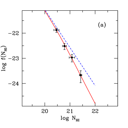
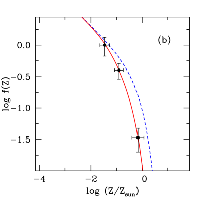
Figure 6: Frequency distributions of of H i column densities (left panel) and metallicities (right panel) in DLAs. Dashed lines: true distributions. Solid lines: distributions biased by quasar obscuration. Circles: empirical distributions obtained from DLA surveys. By imposing that the biased distributions best fit the observed ones, we infer the true distributions (see Section 4.4). The solution shown in the figure was derived for DLAs with a MW-type extinction and quasars observed in the $g^{\prime}$ band.

The effect of DLA extinction on the shape of distribution function of quasar apparent magnitudes can be seen in Fig. 5, where we show the adopted distribution $n_{m}\equiv n(m;z)$ (dashed line) and the predicted biased distribution $n^{\mathrm{b}}_{m}\equiv n^{\mathrm{b}}(m;z)$ (solid line) for the $g^{\prime}$ band and MW-type extinction. The agreement between $n^{\mathrm{b}}_{m}$ and the empirical distribution (diamonds) demonstrates the capability of the procedure to account for the bias in a self-consistent way. The results are very stable for variations of $\pm 0.1$ of the parameter $\overline{\mathcal{F}}_{1}$ around the adopted value $\overline{\mathcal{F}}_{1}=0.5$. Fig. 5 shows that the obscuration effect does not change substantially the shape of the distribution of apparent magnitude of the quasars, at least within the current values of limiting magnitude of the surveys. This is due to the fact that a large fraction of DLAs has relatively low H i column density, as shown in Fig. 6 and, as a consequence, low extinction. The modest bias of the quasar statistics does not imply that the bias is unimportant for the DLAs statistics, as we discuss below.

Fig. 6a is reminiscent of Fig. 8 by FP93 where these authors compare the model and empirical distributions of $N_{\mathrm{H}}$ and $k$. In fact, the dust-to-gas ratios $k$ is defined by FP93 as an extinction per unit H i column density and is therefore almost equivalent to a metallicity, as one can see in our Eq. (11). The fact that the metallicity distribution is much better constrained by the observations than the $k$ distribution is an advantage of our approach. In FP93 the model distribution of $N_{\mathrm{H}}$ is derived using an exponential H i radial profile; in our work the model is meant to be the simplest analytical approximation of the true distribution in the range probed by the observations.

6.1 The H i column density distribution

From the analysis of the H i column density distribution we derive two main results. First, the typical value of $\beta$ that we find, $\beta\simeq 1.5$, is remarkably similar to that measured in quasar absorbers of lower column densities, not affected by obscuration bias (Tytler 1987; Petitjean et al. 1993; Storrie-Lombardi & Wolfe 2000). Second, the biased distribution $f^{\mathrm{b}}_{N_{\mathrm{H}}}$ derived from a simple power law successfully reproduces the shape of the empirical distribution. Both results indicate that the fast decline of the number of absorbers observed in the DLA regime is due to the obscuration effect, the true distribution of column density being instead consistent with a simple power law, as for the majority of quasar absorbers. Quite interestingly, the typical values of $\beta$ that we derive are intermediate between the predictions of the exponential profile model of FP93, $\beta\sim 1$, and the values expected from the mass-spectrum of interstellar clouds, $\beta\ga 2.5$ (see Section 5.2.2). This seems to indicate that both effects should be taken into account in the full theoretical treatment of the true distribution $f_{N_{\mathrm{H}}}$. The hydrodynamic simulations of DLAs by Cen et al. (2003) yield a slope slightly below 2, broadly consistent with our results.

The approximation of the true distribution with a simple power law should not be extrapolated in the range of column densities not sampled by the observations ($\log N_{H\textsc{i}}\raisebox{-5.0pt}{$\;\stackrel{{\scriptstyle\textstyle>}}{{\sim}}\;$}22$). An intrinsic faster decline in that range must occur in order to avoid an infinite value of $\Omega_{\mathrm{DLA}}$ (see Section 6.5). A faster decline is expected in the exponential profile model of disk gas distribution when $N_{H\textsc{i}}$ approaches the central value $N_{\bot 0}$ (FP93). Also the onset of physical mechanisms specific of very high density environments may induce a sharp drop of the distribution at very values of $N_{H\textsc{i}}$ (Schaye 2001). The present results suggest that the genuine fast decline of the $N_{H\textsc{i}}$ distribution may lie beyond the range probed by the observations. In principle, one could model this intrinsic decline with a Schechter function, but the position of the ”knee” would be unconstrained. In the following we introduce an upper cutoff in the column density distribution when we need to estimate quantities affected by the high end of the $N_{H\textsc{i}}$ distribution.

6.2 The metallicity distribution

The results on the metallicity distribution depend on the adopted model for the shape of the distribution. As discussed in Section 5.3, we believe that the results obtained from a Schechter function are more conservative and reliable than those derived from other functions (polynomials, lognormal or other functions parametrized in terms of ”centroid” and ”width”). In addition to the considerations given in Section 5.3 we note here that the position of the ”knee” $Z_{\star}$ is sufficiently well constrained by the observational data (Fig. 6b).

The main result of the analysis of the metallicity distribution is that a non-negligible fraction of DLAs exist with near solar metallicity. In previous work the metallicity distribution of DLAs has been compared with that of different stellar populations of the Milky Way to cast light on the nature of DLA galaxies. Pettini et al. (1997) found that the [Zn/H] distribution observed in DLAs does not resemble that of any Milky-Way population. The true metallicity distribution of DLAs inferred in the present work changes significantly these conclusions. In Fig. 7 we compare the DLA distributions obtained for the best-fit solutions listed in Table 1 with the stellar distributions published by Wyse & Gilmore (1995) for the thick and thin disk of the Milky Way (the same template used by Pettini et al. 1997). One can see that the true DLA distribution envelops those of both disk populations. This result is consistent with the paradigm that DLA galaxies are progenitors of present-day disk galaxies, even though there is plenty of room in the distribution for contributions from metal-poor galaxies. We cannot derive more information from these results because the exact shape of the true distribution is uncertain, particularly in the tails, owing to the poor statistics of the surveys. In any case, the present results bring fresh support to the most commonly accepted paradigm on the nature of DLA galaxies, suggesting that most disks may already be in place at $z\simeq 2.3$, consistent with what happened in the Milky Way.

6.3 The total obscuration fraction

In Table 1 we list the total obscuration $\Phi_{22}$ computed adopting $N_{H\textsc{i}}=10^{22}$ atoms cm^-2 as upper limit of integration in Eq. (17). This is equivalent to truncate the H i distribution in the range of column densities not probed by the observations. The true obscuration factor might be higher than $\Phi_{22}$ if DLA systems exist also beyond such limit. An estimate of this uncertainty can be appreciated in Table 1, where we also give $\Phi_{23}$, obtained integrating the distributions up to $N_{H\textsc{i}}=10^{23}$ atoms cm^-2.

The total obscuration fraction lies in the range $\Phi_{22}\sim 0.33/0.52$ for the magnitude limit typical of high-resolution surveys ($m_{\ell}\sim 19.0$). For spectroscopic surveys of moderate resolution, with $m_{\ell}\sim 19.5$, we obtain $\Phi_{22}\sim 0.27/0.46$. These figures are underestimated by only $\simeq 3/5\%$ if DLAs exist with the same power law, up to $N_{H\textsc{i}}=10^{23}$ atoms cm^-2.

The fraction of missing systems that we find is consistent with the range 0.23 to 0.38 estimated by PF95 at $z\sim 3$.

Our estimate of total obscuration fraction can be compared with that obtained by Ellison et al. (2001) from the analysis of an unbiased sample of radio-selected quasars. By comparing their number density of DLAs, $n(z)$, with that obtained by Storrie-Lombardi & Wolfe (2000) from an optically-selected (biased) sample, Ellison et al. conclude that the unbiased $n(z)$ is about $\sim 50\%$ larger than the biased one. Since the Storrie-Lombardi & Wolfe survey has a magnitude limit typical of moderate resolution surveys, this result should be compared with our obscuration fractions derived for $m_{\ell}=19.5$, which indicate that the true number is between $\sim 40\%$ and $\sim 90\%$ larger than the biased one. The general agreement with the result found by Ellison et al. represents an important test of validity of our procedure.

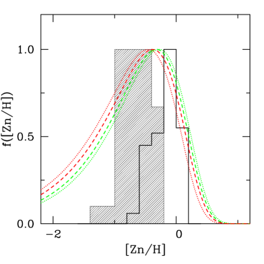
Figure 7: Distribution functions of the logarithmic metallicity normalized to unity. Curves: true distribution of DLAs at $z\simeq 2.3$ inferred with our method. Dashed (dotted) lines: MW-type (SMC-type) extinction; red (green): results for the $r^{\prime}$ ($g^{\prime}$) band. Histograms: Milky-Way stars belonging to the thick disk (shaded area) and thin disk (thick line) populations.

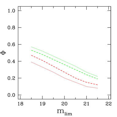
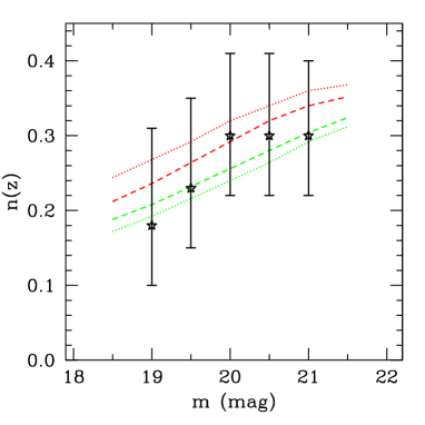
Figure 8: (a) Fraction of obscured DLAs and (b) number density of DLAs predicted as a function of the limiting magnitude for the best-fit solutions of Table 1. Dashed and dotted lines: MW-type and SMC-type extinction, respectively. Red and green: results for the $r^{\prime}$ and $g^{\prime}$ bands. Stars with error bars: CORALS results from Ellison et al. (2001).

6.4 Number density versus limiting magnitude

One prediction of the obscuration bias is that the fraction of missed DLAs must decrease with increasing limiting magnitude of the survey. The variation predicted by our computations is shown in Fig. 8a for the different cases considered in Table 1. The obscured fraction decreases, but does not vanish at least up to $m_{\ell}=21.5$, where $\Phi_{22}\sim 0.1/0.2$. This variation of $\Phi$ versus $m_{\ell}$ offers an important observational test based on the measurement of the number density of DLAs, $n(z)$, at increasing values of $m_{\ell}$ in an unbiased sample. Ellison et al. did find an increase of $n(z)$ with $m_{\ell}$ which supports the existence of the bias. The number density increases in the range $19\la m_{\ell}\la 20$, but flattens at $m_{\ell}\ga 20$, while we predict that it should keep increasing at least up to $m_{\ell}\la 21.5$. However, taking into account the experimental error bars there is no real discrepancy. To demonstrate this, we plot in Fig. 8b $n(z)=n^{\mathrm{t}}(z)\,(1-\Phi)$ for an assumed total density $n^{\mathrm{t}}(z)=0.4$. One can see that these predictions agree with the measurements of $n(z)$ performed by Ellison et al. If $n^{\mathrm{t}}(z)=0.4$, the true number of systems would be $\sim 90\%$ larger than the biased $n(z)$ measured by Storrie-Lombardi & Wolfe. This figure of obscuration is still consistent with our estimate. The only ”disagreement” with Ellison et al. would be on the interpretation of the $n(z)$ versus $m_{\ell}$ plot, for which we claim that there is a steady increase rather than a plateau. More stringent measurements are crucial for clarifyng this issue. It is clear, in any case, that the combination of our treatment of the bias with studies of unbiased samples offers a powerful tool for a quantitative estimate of the obscuration effect.

6.5 The gas content of DLAs

By using our best-fit $N({H\textsc{i}})$ distribution functions we can compute the total contribution of the gas in DLAs to the critical density of the Universe,

$$\Omega_{\mathrm{DLA}}={H_{0}\mu\,m_{\mathrm{H}}\over c\,\rho_{\mathrm{crit}}}\,\int^{\infty}_{N_{\mathrm{min}}}N_{\mathrm{H}}\,f_{N_{\mathrm{H}}}\,dN_{\mathrm{H}}\leavevmode\nobreak\ .$$ (21)

If $f_{N_{\mathrm{H}}}$ is a power law with $\beta<2$, as in our case, the integral diverges and we must introduce an upper cutoff. In Table 1 we give the values $\Omega_{22}$ and $\Omega_{23}$ obtained integrating up to $N_{\mathrm{H}}=10^{22}$ and $10^{23}$ atoms cm^-2, respectively. The value $\Omega_{22}$ is conservative since the true distribution $f_{N_{\mathrm{H}}}$ may extend above $N_{\mathrm{H}}\sim 10^{22}$ cm^-2. The values that we find for different input parameters lie in a relatively narrow range, namely $1.9\times 10^{-3}\leq\Omega_{22}\leq 3.1\times 10^{-3}$.

To estimate the missed fraction of H i mass, we compare these values of $\Omega_{22}$ with $\Omega^{\mathrm{obs}}_{\mathrm{DLA}}\simeq 0.9\times 10^{-3}$, the biased value obtained integrating our H i sample with the commonly adopted Schechter function (19). Since $\Omega_{22}$ is a conservative estimate, this comparison indicates that at $z\sim 2.3$ the true comoving mass of DLAs is at least a factor of 2 higher than that obtained by magnitude-limited surveys.

The values of $\Omega_{22}$ that we derive agree well with the value $\Omega_{\mathrm{E01}}\simeq 2.6\times 10^{-3}$ measured by Ellison et al. (2001) from the analysis of their ”dust-free” sample. In addition, they agree with the value $\Omega_{\mathrm{DLA}}\simeq 3\times 10^{-3}$ derived at $z\simeq 2.3$ by Cen et al. (2003) from their hydrodynamic simulations.

6.6 The metal content of DLAs

The column-density weighted metallicity of DLA systems is used to measure the degree of metal enrichment of the population of DLAs as a whole (Pettini et al. 1999) and to estimate the mean cosmic metallicity of the high-redshift Universe (Pei & Fall 1995; Cen et al. 2003). The expression commonly used in literature to measure the weighted metallicity from a finite set of column densities, $<\!(\mathrm{Zn/H})_{\mathrm{DLA}}\!>={(\sum_{i}N_{\mathrm{Zn},i})/(\sum_{i}N_{\mathrm{H},i})}$, can be put in the form

$$<\!(\mathrm{Zn}/\mathrm{H})_{\mathrm{DLA}}\!>={\int N_{\mathrm{Zn}}\leavevmode\nobreak\ f_{N_{\mathrm{Zn}}}\leavevmode\nobreak\ dN_{\mathrm{Zn}}\over\int N_{\mathrm{H}}\leavevmode\nobreak\ f_{N_{\mathrm{H}}}\leavevmode\nobreak\ dN_{\mathrm{H}}}\leavevmode\nobreak\ ,$$ (22)

to measure the same quantity from the frequency distribution functions $f_{N_{\mathrm{Zn}}}$ and $f_{N_{\mathrm{H}}}$ normalized to unit area. If the metallicity $Z$ and the H i column density are independent variables, as we assume in our mathematical formulation, then it is easy to show that $<\!(\mathrm{Zn/H})_{\mathrm{DLA}}\!>$ equals the expectation value $<\!Z\!>=\int Z\leavevmode\nobreak\ f_{Z}\leavevmode\nobreak\ d\,Z$ estimated from the distribution $f_{Z}$ normalized to unit area.

In Table 1 we list the mean metallicity, normalized in the usual form $\log(<\!Z\!>/Z_{\sun})$, obtained for a Schechter metallicity distribution. The mean metallicity lies between $-0.44$ and $-0.27$ dex below the solar level for the different dust models and photometric bands considered in Table 1. Considering the total error of $\sim-0.3$ dex in our estimate (fit errors plus statistical errors of the empirical distributions) we conclude that the mean metallicity is $\raisebox{-5.0pt}{$\;\stackrel{{\scriptstyle\textstyle>}}{{\sim}}\;$}-0.7$ dex at 1 $\sigma$ level. These values are higher than the direct measurements of weighted metallicity of DLAs, which give $\sim-1.1$ dex at the typical redshift of our sample (Pettini et al. 1999; Prochaska et al. 2003). This large difference is probably be due to the fact that the weighted metallicity is extremely sensitive to the number of high column-density DLAs included in the average, which are the DLAs more affected by obscuration. Our results are marginally consistent with the mean weighted metallicity $\left[<\!\mathrm{(Zn/H)_{DLA}}\!>\right]=-0.88\pm 0.21$ dex obtained from the CORALS metallicity survey (Akerman et al. 2005).

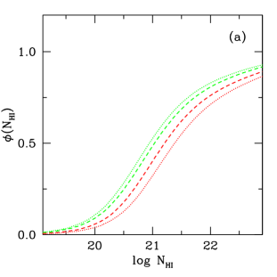
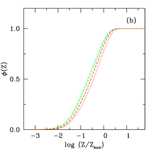
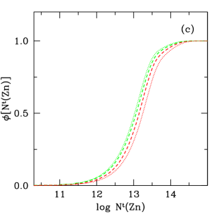
Figure 9: Fraction of obscured DLAs as a function of (a) H i column density, (b) metallicity $Z$, and (c) Zn ii column density for the best-fit solutions of Table 1. Dashed and dotted lines: caption as in Fig. 8.

Quite interestingly, the high mean metallicity that we derive may help to solve the ”missing metal” problem pointed out by Wolfe et al. (2003) in their work on the Star Formation Rates (SFRs) in DLAs: the mass of metals produced by $z\simeq 2.5$, inferred from their SFRs, is 30 times larger than detected in absorption in DLAs.

6.7 Observational thresholds due to obscuration bias

Our method allows us to estimate, for the first time, the fraction of obscured DLAs as a function of H i column density and metallicity $Z$, and also as a function of the total zinc column density. These obscuration fractions $\phi_{\ell}(N_{\mathrm{H}})$, $\phi_{\ell}(Z)$ and $\phi_{\ell}(N^{\mathrm{t}}_{\mathrm{Zn}})$, shown in Fig. 9, should only be interpreted in a statistical sense. However, they provides us a powerful indication of how the statistical distributions of DLAs are distorted by the obscuration bias. In particular, they provide a means of quantifying the existence of observational cutoffs induced by the bias itself.

The analysis of $\phi_{\ell}(N^{\mathrm{t}}_{\mathrm{Zn}})$, shown in panel (c), gives a quantitative explanation for the lack of DLAs systems above the obscuration threshold in Zn ii column density originally proposed by Boissé et al. (1998). We estimate that over $60\%$ of DLAs are missed at $N^{\mathrm{t}}_{\mathrm{Zn}}=10^{13.2}$ atoms cm^-2, and this fraction rises rapidly to $\sim 95\%$ if the $N^{\mathrm{t}}_{\mathrm{Zn}}$ increases by $\simeq 0.5$ dex. The threshold is rather independent of the adopted input parameters. Only for peculiar extinction curves without UV rise (gray extinction) we may expect that the threshold can be crossed.

We can use our results to estimate how many DLAs should be observed in an unbiased survey in order to detect cases with high metal column density. From the typical distribution $f_{N_{\mathrm{Zn}}}$ that we infer, we estimate that the number of DLAs in the range between the detection limit and the Boissé’s threshold ($11.5\raisebox{-5.0pt}{$\;\stackrel{{\scriptstyle\textstyle<}}{{\sim}}\;$}\log N({Zn\textsc{ii}})\raisebox{-5.0pt}{$\;\stackrel{{\scriptstyle\textstyle<}}{{\sim}}\;$}13.1$) is about 24 times larger than the number of systems in a range of similar extension above the threshold ($13.1<\log N({Zn\textsc{ii}})\raisebox{-5.0pt}{$\;\stackrel{{\scriptstyle\textstyle<}}{{\sim}}\;$}14.7$). This means that one is not guaranteed to detect one DLA above the threshold even with $\sim 30$ unbiased spectroscopic observations. This is currently an observational challenge because the high extinction of the DLAs above the threshold makes very hard to perform high-resolution spectroscopy, even for the quasars which lie at the bright end of the true distribution of apparent magnitudes.

A natural consequence of the cutoff at high metal column densities, in conjunction with the artificial DLA threshold $N_{H\textsc{i}}\geq 10^{20.3}$ atoms cm^-2, is the existence of an observational cutoff at high metallicities. From panel (b) one can see that about $90\%$ of systems are missed at solar metallicity and it would be practically impossible to detect systems with oversolar metallicity, if they exist. Also worth of mention is the fast rise of the obscuration with increasing metallicity, which distorts dramatically our perception of the metallicity distribution of DLA systems. The fact the different curves plotted in panel (b) lie close to each other indicates that these results are rather independent of the parameters adopted.

Also the distribution of H i column densities is severely distorted by the extinction bias, as shown in panel (a). The curves of $\phi(N_{\mathrm{H}})$ obtained for different parameters are not tightly close to each other, but the general behaviour is quite similar in all cases. The obscuration starts from a low value in the sub-DLA regime and rises steadily over the DLA regime, approaching $\sim 80\%$ at $N_{H\textsc{i}}\sim 10^{22}$ atoms cm^-2. This is the approximate value of the observational threshold for detection of high column density DLAs. The rise of $\phi(N_{\mathrm{H}})$, in conjunction with the genuine decrease of the true distribution $f_{N_{\mathrm{H}}}$, provides a natural explanation for the non-detection of DLAs at $N_{H\textsc{i}}\ga 10^{22}$ atoms cm^-2. This makes it unnecessary to invoke the sudden transition from atomic to molecular hydrogen proposed by Schaye (2001) in order to explain this empirical cutoff. In any case, if fully molecular clouds exist as predicted by Schaye, they would be characterized by a high column density of dust grains. The fact that quasar absorbers with $N(\mathrm{H_{2}})>N({H\textsc{i}})$ have not yet been detected may indicate that also this type of absorber is missed due to obscuration.

7 Summary and conclusions

Starting from the theoretical relation between the interstellar extinction, $A_{\lambda}$, and the column density of a volatile metal, $N_{\mathrm{X}_{v}}$, we investigated the detailed relation between $A_{\lambda}$ and $N_{\mathrm{Zn}}$ in DLAs. We derived in this way the Eq. (11), which gives the quasar extinction in the observer’s frame as a function of the DLA hydrogen column density, $N_{\mathrm{H}}$, metallicity, $Z=N_{\mathrm{Zn}}/N_{\mathrm{H}}$, fraction in dust of iron, $f_{\mathrm{Fe}}$, and a factor $G$, which describes the dust grain properties. For the first time, the metallicity evolution of the dust-to-metal ratio in DLAs is explicitly accounted for in this type of relation, using an expression $f_{\mathrm{Fe}}=f_{\mathrm{Fe}}(Z)$ obtained from a previous study of depletions (Vladilo 2004). We argue that the factor $G$ may not vary substantially in interstellar environments with moderately low metallicity ($Z\ga 0.1\,Z_{\sun}$) and derive a value of 60% the Milky-Way value for SMC-type dust. Possible variations of $G$ at the early stages of chemical evolution do not affect the extinction because $f_{\mathrm{Fe}}(Z)$ vanishes when $Z\ll Z_{\sun}$.

We searched for empirical evidence of the rise of the extinction with metal column density in DLAs. We did find an increase of the quasar magnitude with $N_{\mathrm{Zn}}$, consistent with this expectation (Fig. 4).

Starting from Eq. (11), we derived a mathematical formulation aimed at estimating how the frequency distributions of H i column densities and metallicities of a sample of DLAs are biased as a result of the obscuration generated by the DLAs of the same sample. We ignore the obscuration due to low-redshift DLAs along the same line of sight, showing that this contribution is relatively low. At variance with the formulation of PF95, where a constant dust-to-metal ratio was adopted for all DLAs, we adopted a metal-dependent dust-to-metal ratio $f_{\mathrm{Fe}}(Z)$. We cross-checked the validity of our formulation making use of the equations derived by FP93 for the case of a power law quasar luminosity function and constant dust-to-gas ratio (Section A.1.2).

We presented a practical procedure for recovering the unbiased distributions of column densities and metallicities, $f_{N_{\mathrm{H}}}$ and $f_{Z}$, using the empirical distributions obtained from magnitude-limited surveys. The unbiased distributions are modelled with simple analytical expressions in parametric form. The bias induced by the extinction on the quasar magnitude distribution is accounted for self-consistently by the procedure. A unique characteristic of the method is the possibility of recovering the true metallicity distribution starting from an educated guess of the functional form of the distribution. We have shown that using a Schechter function for the metallicity distribution appears to provide more conservative and reliable results than other functions (e.g. lognormal or polynomials) for the estimate of the bias (Section 5.3).

We applied our method to the sample of DLAs in the redshift interval $1.8\leq z\leq 3$, with mean redshift $<\!\!z\!\!>\simeq 2.3$, where the bulk of spectra are available. The extinctions were computed in the $g^{\prime}$ and $r^{\prime}$ photometric bands of the SDSS, considering both a MW-type and an SMC-type average extinction curve. We found that the effect of the obscuration on the quasar magnitude distribution is modest (e.g. Fig. 5). On the other hand, the bias plays an important role in shaping the statistical distributions of DLAs.

The unbiased distribution function of H i column densities is successfully approximated by a power law $f_{N_{\mathrm{H}}}\propto N_{\mathrm{H}}^{-\beta}$, with $\beta\simeq 1.5$. This simple law, in conjunction with the bias effect, is able to fit the observed decline of the number DLAs with $N_{\mathrm{H}}$ up to $N({H\textsc{i}})\sim 10^{21.8}$ atoms cm^-2. The faster drop of the distribution expected at very high column densities (FP93; Schaye 2001) probably lies outside the range currently probed by the observations. The slope $\beta\simeq 1.5$ is remarkably similar to the value which characterizes most of quasars absorbers with lower column densities, for which the extinction bias is negligible. The value of the slope suggests that the mass spectrum of interstellar clouds may play an important role in shaping the distribution.

The observed distribution of metallicities is reproduced modelling the unbiased distribution with a Schechter function $f_{Z}\leavevmode\nobreak\ \propto\leavevmode\nobreak\ (Z/Z_{\ast})^{\alpha}\leavevmode\nobreak\ e^{-Z/Z_{\ast}}$, with $\alpha\simeq-0.4$ and $\log(Z_{\ast}/Z_{\sun})\simeq-0.15$ dex. Once converted into logarithmic scale, this function peaks at [Zn/H] $\sim-0.3/-0.4$ dex, indicating that a non-negligible fraction of DLAs exist with near solar metallicity. The true metallicity distribution of DLAs envelops the distributions of the thick-disk and thin-disk Milky-Way stellar populations. This result is in line with the paradigm that DLA galaxies are progenitors of present-day disk galaxies. However, in the inferred distribution there is also room for a relevant contribution from metal-poor galaxies.

The mean weighted metallicity that we derive , $\simeq-0.4/\!-0.3$ dex, is significantly higher than the column-density weighted metallicity $<\!\!\mathrm{[Zn/H]}\!\!>=-1.1$ dex measured at $z\simeq 2.3$. This high value of mean metallicity may help to solve the discrepancy between the metallicity observed in DLAs and that predicted on the basis of their SFRs (Wolfe et al. 2003).

The fraction by number of obscured DLAs, $\Phi$, decreases with increasing limiting magnitude of the survey, $m_{\ell}$. We obtain $\Phi\ga 0.4/0.6$ at $m_{\ell}\la 18.5$, a limit representative of high resolution spectroscopic surveys, carried out with 4-m class telescopes. The corresponding figures for high-resolution surveys in 10-m class telescopes are $\Phi\simeq 0.35/0.55$ ($m_{\ell}\simeq 19.0$).

An important result of our work is the explanation (Fig. 9c) of the observational limit $N_{\mathrm{Zn}}\sim 10^{13.2}$ atoms cm^-2 (Boissé et al. 1998) in terms of very simple physics (Section 2), with no tuning of the local dust parameters. Alternative explanations would require an additional mechanism able to produce the exact same limit predicted by the extinction. The simplicity of the extinction model favours the existence of the obscuration. The existence of the threshold $N_{\mathrm{Zn}}\sim 10^{13.2}$ atoms cm^-2 is fundamental for reconciling the predictions of galactic models (Prantzos & Boissier 2000, Hou et al. 2001; Churches et al. 2004) and cosmological simulations (Cen et al. 2003, Nagamine et al. 2004) with the observations of DLAs. Only for gray extinction curves, without UV rise, we may expect that the threshold can be crossed.

Our results on the magnitude of the obscuration effect are broadly consistent with those presented by FP93 and PF95, with some important differences. The modest bias of quasar statistiscs that we find is at variance with the predictions of FP93, which allowed up to 70% of quasars to be obscured. Contrary to FP93, we do not expect a significant contribution of DLA extinction at redshift $z\raisebox{-5.0pt}{$\;\stackrel{{\scriptstyle\textstyle>}}{{\sim}}\;$}3$ in spite of the rise of $A_{\lambda}$ with $z$. In fact, our model of dust fraction $f_{\mathrm{Fe}}(Z)$ vanishes at very low metallicity so that the extinction (11) vanishes at $z\raisebox{-5.0pt}{$\;\stackrel{{\scriptstyle\textstyle>}}{{\sim}}\;$}3$, when the metallicity $Z\raisebox{-5.0pt}{$\;\stackrel{{\scriptstyle\textstyle<}}{{\sim}}\;$}0.01Z_{\sun}$.

A crucial test of our results is the comparison with studies of radio-selected samples of quasars/DLAs. Our determinations are consistent with the estimates of obscuration fraction, number density and $\Omega_{\mathrm{DLA}}$ obtained from the CORALS survey (Ellison et al. 2001). Our prediction of mean metallicity is marginally consistent with the recent estimate of mean weighted metallicity of the CORALS sample (Akerman et al. 2005).

Accurate estimates of the obscuration effect will be possible as soon as the samples with metallicity measurements become sufficiently large for precise statistical analysis.

Appendix A Mathematical formulation

A.1 True and biased distributions

To derive our mathematical formulation we define the frequency distributions of DLAs and quasars most appropriate for taking into account the causes and effects of the extinction bias. To account for the DLA extinction via Eq. (11) we are interested in the number of DLAs per unit hydrogen column density and metallicity. To account for the dimming of the quasar we are interested in the number of quasars per unit of apparent magnitude. The apparent magnitude, $m$, can be directly compared with the limiting magnitude of the observational survey, $m_{\ell}$.

We call $h(N_{\mathrm{H}},Z,z)\,dN_{\mathrm{H}}\,dZ\,dz\,d\omega$ the number of neutral hydrogen layers with column density $N_{\mathrm{H}}\in(N_{\mathrm{H}},N_{\mathrm{H}}+dN_{\mathrm{H}})$ and metallicity $Z\in(Z,Z+d\,Z)$ located in the spherical shell of redshift $z\in(z,z+dz)$ in the infinitesimal solid angle $d\omega$ in a random direction (we assume that the gas layers are distributed isotropically).

We call $q(m,z_{e})\,dm\,dz_{e}$ the true number of quasars with apparent magnitude $m\in(m,m+dm)$ in the shell of emission redshift $z_{e}\in(z_{e},z_{e}+dz_{e})$ all over the sky (we assume an isotropic distribution of quasars). We define $n(m;z,z_{e}^{\mathrm{max}})\equiv\int_{z}^{z_{e}^{\mathrm{max}}}q(m,z_{e})\,dz_{e}$, where $z$ is the absorption redshift of a foreground H i layer and $z_{e}^{\mathrm{max}}$ the maximum redshift of the quasars in the survey. For simplicity of notation we omit hereafter the dependence on $z_{e}^{\mathrm{max}}$. Therefore $n(m;z)\,dm$ is the total number of quasars with magnitude $m\in(m,m+dm)$ observable beyond redshift $z$ all over the sky. This is the true number in absence of quasar obscuration.

We call $\delta\omega_{\mathrm{q}}(z)$ the average solid angle subtended in the observer’s optical band by quasars in the redshift interval $z<z_{e}\leq z_{e}^{\mathrm{max}}$.

With the above definitions, the number of DLAs with $N_{\mathrm{H}}\in(N_{\mathrm{H}},N_{\mathrm{H}}+dN_{\mathrm{H}})$, $Z\in(Z,Z+d\,Z)$ and redshift $z\in(z,z+dz)$ in front of one single background quasar with $m\leq m_{\ell}$ is

$$h(N_{\mathrm{H}},Z,z)\,dN_{\mathrm{H}}\,dZ\,dz\,\delta\omega_{\mathrm{q}}(z)$$

provided $N_{\mathrm{H}}=N({H\textsc{i}})\geq 10^{20.3}$ atoms cm^-2. The number of DLAs in the same differential element $dN_{\mathrm{H}}\,dZ\,dz$ that are detectable in front of the $n(m;z)\,dm$ background quasars with $m\in(m,m+dm)$ is

$$h(N_{\mathrm{H}},Z,z)\,dN_{\mathrm{H}}\,dZ\,dz\,\delta\omega_{\mathrm{q}}(z)\times\,n(m;z)\,dm\,,$$

provided $m\leq m_{\ell}$. By integrating in $dm$ up to the limiting magnitude $m_{\ell}$ we calculate the total number of DLAs that are detectable in the survey. We first consider the ideal case in which no quasar extinction is present. In this case the unbiased number of detectable DLAs in $dN_{\mathrm{H}}\,dZ\,dz$ is

$$g_{m_{\ell}}(N_{\mathrm{H}},Z,z)\,dN_{\mathrm{H}}\,dZ\,dz\equiv{}$$ (23)

$${}h(N_{\mathrm{H}},Z,z)\,\delta\omega_{\mathrm{q}}(z)\left[\int_{\circ}^{m_{\ell}}n(m;z)\,dm\right]dN_{\mathrm{H}}\,dZ\,dz\,.$$

We call $g_{m_{\ell}}(N_{\mathrm{H}},Z,z)$ the true distribution of detectable DLAs in $dN_{\mathrm{H}}\,dZ\,dz$.

We then consider the quasar extinction $A_{\lambda}(N_{\mathrm{H}},Z;z)$ due to the DLAs in $dN_{\mathrm{H}}\,dZ\,dz$ (Eq. 11) ignoring other sources of extinction. From this we define the bias function

$$b_{m_{\ell}}(N_{\mathrm{H}},Z,m,z)\equiv\left\{\begin{array}[]{ll}1&\leavevmode\nobreak\ \leavevmode\nobreak\ \mbox{if $m\leq{m}_{\ell}-A_{\lambda}(N_{\mathrm{H}},Z;z)$ }\\ 0&\leavevmode\nobreak\ \leavevmode\nobreak\ \mbox{if $m>{m}_{\ell}-A_{\lambda}(N_{\mathrm{H}},Z;z)$ }\\ \end{array}\leavevmode\nobreak\ .\right.$$ (24)

The number of DLAs in $dN_{\mathrm{H}}\,dZ\,dz$ that, in spite of their own extinction, are detectable in front of the $n(m;z)\,dm$ background quasars is

$$b_{m_{\ell}}(N_{\mathrm{H}},Z,m,z)\,h(N_{\mathrm{H}},Z,z)\,dN_{\mathrm{H}}\,dZ\,dz\,\delta\omega_{\mathrm{q}}(z)\,n(m;z)\,dm.$$

By integrating in $dm$ we obtain the total number of DLAs in $dN_{\mathrm{H}}\,dZ\,dz$ that, in spite of their own extinction, are detectable in the survey

$$g_{m_{\ell}}^{\mathrm{b}}(N_{\mathrm{H}},Z,z)\,dN_{\mathrm{H}}\,dZ\,dz\equiv h(N_{\mathrm{H}},Z,z)\,\delta\omega_{\mathrm{q}}(z)\times{}$$ (25)

$$\times\left[\int_{\circ}^{m_{\ell}-A_{\lambda}(N_{\mathrm{H}},Z,z)}\,n(m;z)\,dm\right]dN_{\mathrm{H}}\,dZ\,dz\,.$$

The number of DLAs in the survey that are missed as a consequence of their own extinction is $\left(g_{m_{\ell}}-g_{m_{\ell}}^{\mathrm{b}}\right)\,dN_{\mathrm{H}}\,dZ\,dz$. The fraction of DLAs missed as a consequence of their own extinction is

$$\varphi_{m_{\ell}}(N_{\mathrm{H}},Z,z)\,\equiv{g_{m_{\ell}}-g_{m_{\ell}}^{\mathrm{b}}\over g_{m_{\ell}}}=1-B_{m_{\ell}}(N_{\mathrm{H}},Z,z)\,,$$ (26)

where

$$B_{m_{\ell}}(N_{\mathrm{H}},Z,z)\equiv{\int_{\circ}^{m_{\ell}-A_{\lambda}(N_{\mathrm{H}},Z,z)}\,n(m;z)\,dm\,\over\int_{\circ}^{m_{\ell}}\,n(m;z)\,dm}\,.$$ (27)

The ratio of the integrals of the magnitude distribution in Eq. (27) is reminiscent of the ratio of the integrals of the quasar luminosity function in Eq. (3) of FP93. This ratio represents, in a sense, the core relation from which the bias effect is estimated.

The relation between the true distribution and the distribution biased by its own DLAs is

$$g_{m_{\ell}}^{\mathrm{b}}(N_{\mathrm{H}},Z,z)=B_{m_{\ell}}(N_{\mathrm{H}},Z,z)\leavevmode\nobreak\ g_{m_{\ell}}(N_{\mathrm{H}},Z,z)\,.$$ (28)

This relation is independent of the average solid angle $\delta\omega_{\mathrm{q}}(z)$. The normalization factor of $n(m,z)$ is also irrelevant because it is eliminated in Eq. (27).

To make practical use of Eq. (28) we need to understand the relation between the biased distribution $g_{m_{\ell}}^{\mathrm{b}}(N_{\mathrm{H}},Z,z)$ and the observed distribution of DLAs in $dN_{\mathrm{H}}\,dZ\,dz$, that we call $g_{m_{\ell}}^{\mathrm{obs}}(N_{\mathrm{H}},Z,z)$. To derive an expression for the observed distribution we must consider all the sources of obscuration, including the DLAs at $z^{\prime}<z$ that lie in the same lines of sight of the DLAs at redshift $z$. If these additional sources of obscuration are negligible, then the expression (28) is a good approximation of the observed distribution (see A.1.1), i.e.

$$g_{m_{\ell}}^{\mathrm{obs}}(N_{\mathrm{H}},Z,z)\simeq g_{m_{\ell}}^{\mathrm{b}}(N_{\mathrm{H}},Z,z)\,.$$ (29)

Using the above approximation, the treatment of the obscuration bias is self-contained, in the sense that given the true distributions of column densities and metallicities at a redshift $z$, the observed distributions of the same quantities are uniquely determined. In this way we can study the obscuration effect in a redshift interval sampled by the observations, even if we do not have good statistics of the DLAs at lower redshifts.

To compare the distributions with the observations we integrate Eq. (28) in $dz$ over the interval $(z_{\mathrm{min}},z_{\mathrm{max}})$ with $\overline{z}=(z_{\mathrm{max}}-z_{\mathrm{min}})/2$ close to the peak of the observed distribution. If the statistical functions of interest show a smooth variation inside the interval we can approximate them with their value at $z=\overline{z}$. We obtain

$$f^{\mathrm{b}}(N_{\mathrm{H}},Z)\simeq\mathcal{B}_{m_{\ell}}(N_{\mathrm{H}},Z)\leavevmode\nobreak\ f(N_{\mathrm{H}},Z)\leavevmode\nobreak\ ,$$ (30)

where

$$f^{\mathrm{b}}(N_{\mathrm{H}},Z) \equiv \int_{z_{\mathrm{min}}}^{z_{\mathrm{max}}}g^{\mathrm{b}}(N_{\mathrm{H}},Z,z)\ dz$$

$$f(N_{\mathrm{H}},Z)\leavevmode\nobreak\ \equiv \int_{z_{\mathrm{min}}}^{z_{\mathrm{max}}}g(N_{\mathrm{H}},Z,z)\ dz$$ (31)

and

$$\mathcal{B}_{m_{\ell}}(N_{\mathrm{H}},Z)\equiv B_{m_{\ell}}(N_{\mathrm{H}},Z,\overline{z})\leavevmode\nobreak\ .$$ (32)

For simplicity we omit the dependence of these functions on $\overline{z}$, $z_{\mathrm{min}}$ and $z_{\mathrm{max}}$.

We now transform the distribution $f(N_{\mathrm{H}},Z)$ into a distribution of column densities, $f_{N_{\mathrm{H}}}$, and a distribution of metallicities, $f_{Z}$, defined in such a way that $f_{N_{\mathrm{H}}}dN_{\mathrm{H}}$ is the true number of detectable DLAs with column densities between $N_{\mathrm{H}}$ and $N_{\mathrm{H}}+dN_{\mathrm{H}}$ in the interval $(z_{\mathrm{min}},z_{\mathrm{max}})$ and $f_{Z}\,dZ$ the true number of detectable DLAs with metallicity between $Z$ and $Z+d\,Z$ in the same redshift interval. We call $f^{\mathrm{b}}_{N_{\mathrm{H}}}$ and $f^{\mathrm{b}}_{Z}$ the corresponding biased distribution functions.

To proceed further we assume that $N_{\mathrm{H}}$ and $Z$ are independent variables (this assumption is discussed in Section 4.4). This implies that $f(N_{\mathrm{H}},Z)\,dN_{\mathrm{H}}\,d\,Z=f_{N_{\mathrm{H}}}\,dN_{\mathrm{H}}\,f_{Z}\,d\,Z$. We substitute this expression in the right hand of Eq. (30). We then integrate that equation in metallicity and obtain

$$\int_{0}^{\infty}f^{\mathrm{b}}(N_{\mathrm{H}},Z)\,dZ\simeq\left[\int_{0}^{\infty}\mathcal{B}_{m_{\ell}}(N_{\mathrm{H}},Z)\,f_{Z}\,d\,Z\right]\leavevmode\nobreak\ f_{N_{\mathrm{H}}}\leavevmode\nobreak\ \leavevmode\nobreak\ .$$ (33)

Apart from a constant factor, the left term of this equation represents the biased distribution $f^{\mathrm{b}}_{N_{\mathrm{H}}}$. The constant can be determined by imposing that in absence of bias the true and biased distributions must be equal. From this we derive the relation

$$f^{\mathrm{b}}_{N_{\mathrm{H}}}\simeq{\int_{0}^{\infty}\mathcal{B}_{m_{\ell}}(N_{\mathrm{H}},Z)\,f_{Z}\,d\,Z\over\int_{0}^{\infty}f_{Z}\,d\,Z}\leavevmode\nobreak\ f_{N_{\mathrm{H}}}\leavevmode\nobreak\ \leavevmode\nobreak\ .$$ (34)

In a similar way, by integrating Eq. (30) in $dN_{\mathrm{H}}$, we obtain the relation

$$f^{\mathrm{b}}_{Z}\simeq{\int_{N_{\mathrm{DLA}}}^{\infty}\mathcal{B}_{m_{\ell}}(N_{\mathrm{H}},Z)\,f_{N_{\mathrm{H}}}\,d\,N_{\mathrm{H}}\over\int_{N_{\mathrm{DLA}}}^{\infty}f_{N_{\mathrm{H}}}\,d\,N_{\mathrm{H}}}\leavevmode\nobreak\ f_{Z}\leavevmode\nobreak\ \leavevmode\nobreak\ ,$$ (35)

where $N_{\mathrm{DLA}}=10^{20.3}$ atoms cm^-2.

A.1.1 Condition of validity of Eq. (29)

We start by deriving the relation between the true number of detectable DLAs in absence of obscuration, $g_{m_{\ell}}(N_{\mathrm{H}},Z,z)\,dN_{\mathrm{H}}\,dZ\,dz$, and the number observed when all sources of obscuration are considered, $g_{m_{\ell}}^{\mathrm{obs}}(N_{\mathrm{H}},Z,z)\,dN_{\mathrm{H}}\,dZ\,dz$.

At redshift $z$ the observed number equals the true number minus the fraction of DLAs missed as a consequence of their own extinction, $\varphi=\varphi_{m_{\ell}}(N_{\mathrm{H}},Z,z)$, minus the fraction of DLAs at redshift $z$ missed due to the extinction of other DLAs at $z^{\prime}<z$ that lie in the same line of sight, $\varphi^{\prime}=\varphi_{m_{\ell}}^{\prime}(N_{\mathrm{H}},Z,z)$. This implies

$$g_{m_{\ell}}^{\mathrm{obs}}(N_{\mathrm{H}},Z,z)=g_{m_{\ell}}(N_{\mathrm{H}},Z,z)\times\left(1-\varphi-\varphi^{\prime}\right)\,.$$ (36)

In the term $\varphi^{\prime}$ we should not count the DLAs at redshift $z$ that are missed due to their own extinction, since they are already counted in the term $\varphi$. We should instead count only the fraction $\left(1-\varphi\right)$ of DLAs at redshift $z$ that are not missed due to their own extinction. Of this residual fraction, we must in turn take the fraction of DLAs at redshift $z$ that have an additional DLA at $z^{\prime}<z$ in the same line of sight, $F(z^{\prime},z)$. Of the resulting fraction, we must finally consider the mean fraction of DLAs at redshift $z^{\prime}<z$ that are missed due to their own extinction, $\overline{\varphi}(z^{\prime}\!\!<\!z)$. From these considerations we obtain the relation

$$\varphi^{\prime}=\left(1-\varphi\right)\times F(z^{\prime},z)\times\overline{\varphi}(z^{\prime}\!\!<\!z).$$ (37)

From Eqs. (26) and (28) we have $g_{m_{\ell}}^{\mathrm{b}}(N_{\mathrm{H}},Z,z)=g_{m_{\ell}}(N_{\mathrm{H}},Z,z)\times\left(1-\varphi\right)$. Comparing with Eq. (36) one can see that the approximation of Eq. (29), $g_{m_{\ell}}^{\mathrm{obs}}(N_{\mathrm{H}},Z,z)\simeq g_{m_{\ell}}^{\mathrm{b}}(N_{\mathrm{H}},Z,z)$, is valid when

$$\varphi^{\prime}\ll 1-\varphi$$ (38)

By combining Eq. (37) with (38) we obtain that

$$F(z^{\prime},z)\times\overline{\varphi}_{m_{\ell}}(z^{\prime}\!\!<\!z)\ll 1$$ (39)

describes the limits of validity of the approximation (29). We estimate the validity of this condition at $z\simeq 2.3$, the mean absorption redshift of the surveys.

From a recent summary (Ellison et al. 2004) of the unbiased number density of DLAs, $n_{\mathrm{DLA}}(z)$, we calculate that the probability of intersecting 2 DLAs in a random line of sight up to $z\simeq 2.3$ is $\approx 0.15$. We take this value as an estimate of $F(z^{\prime},z)$.

By comparing the number densities of biased and unbiased surveys there is room for no more than $\approx 50\%$ of missed DLAs at $z\simeq 2.3$ (Ellison et al. 2001, 2004). This represents an upper limit to $\overline{\varphi}_{m_{\ell}}(z^{\prime}<2.3)$ because the extinction in the observer’s frame tends to decrease with decreasing redshift and therefore the missed fraction ${\varphi}_{m_{\ell}}(z^{\prime}<z)$ tends to diminish at lower redshifts.

All together, we expect therefore $F(z^{\prime},z)\times\overline{\varphi}_{m_{\ell}}(z^{\prime}<z)\la 0.08$ at $z\simeq 2.3$ and lower values at lower redshifts. We conclude that the approximation (29) is good, even if it may slightly underestimate the obscuration fraction.

A.1.2 Test of Eqs. (27), (28) and (34)

To test our formulation we cross-checked its predictions in a particular case considered by Fall & Pei (1993). Namely, we compared the predictions of our Eq. (28), calculated at constant metallicity $Z$, with those of Eq. (21) by FP93, which is calculated at a constant dust-to-gas ratio $k$. This test is equivalent to insert in Eq. (34) a Dirac delta distribution of metallicities. To make this comparison we transformed the power-law distribution of quasar luminosities used by FP93 [their Eq. (8)] into a magnitude distribution $n(m;z)$ for our Eq. (27). We adopted $\beta=2$ and $\xi({\lambda\over 1+z})=2.78$ as common values in both equations. In Eq. (21; FP93) we adopted a value of $k=0.04$ consistent with our choice of $G=1$, $Z/Z_{\sun}=0.1$ and $f_{\mathrm{Fe}}(Z)=0.52$ for this particular test. In Fig. 10 we compare the resulting ratio $f_{o}(N,z)/f_{t}(N,z)$ predicted from Eq. (21) by FP93 with the corresponding ratio $g_{m_{\ell}}^{\mathrm{b}}(N_{\mathrm{H}},Z,z)/g_{m_{\ell}}(N_{\mathrm{H}},Z,z)$ predicted from our Eq. (28), which equals the term $B_{m_{\ell}}(N_{\mathrm{H}},Z,z)$ of Eq. (27). Our predictions (empty circles) perfectly match those obtained with the equations derived by FP93 (filled diamonds). Our results are independent of $m_{\ell}$ provided $m_{\ell}\gg 1$ and $m_{\ell}\gg A_{\lambda}$. For $m_{\ell}\approx 19$ - $20$ these conditions are well satisfied.

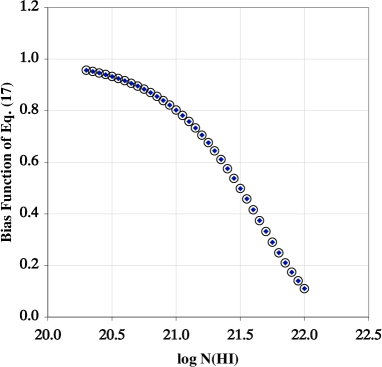
Figure 10: A test of validity of the equations presented in Section 4.1. Circles: predictions of our Eq. (27). Diamonds: $f_{o}(N,z)/f_{t}(N,z)$ predicted from Eq. (21) by Fall & Pei (1993). The adopted parameters are given in Appendix A.1.2.

A.2 The quasar magnitude distribution

We derive the relation between the ”true” magnitude distribution of quasars, $n(m;z)$, and the observed one, which is biased by the obscuration effect. We consider only the obscuration due to DLA systems. We start by defining $q^{\mathrm{b}}(m,z_{e})\,dm\,dz_{e}$ the observed (biased) number of quasars with magnitude $m\in(m,m+dm)$ at redshift $z_{e}\in(z_{e},z_{e}+dz_{e})$. We then divide the quasars according to the number $i$ of DLAs that lie in their direction. We call $\mathcal{F}_{i}(z_{e})$ the fraction of quasars at redshift $z_{e}$ that have $i$ intervening DLAs. Depending on the value of $i$, the distribution of apparent magnitudes of the quasars will be different. We call $q^{\mathrm{b}}_{i}(m,z_{e})\,dm\,dz_{e}$ the biased number of quasars with $i$ foreground DLAs, magnitude $m\in(m,m+dm)$ and redshift $z_{e}\in(z_{e},z_{e}+dz_{e})$. We now assume that the fraction of quasars with two or more DLAs is negligible (see A.1.1), i.e. that $\mathcal{F}_{i\geq 2}(z_{e})\ll\mathcal{F}_{0}(z_{e})$ and $\mathcal{F}_{i\geq 2}(z_{e})\ll\mathcal{F}_{1}(z_{e})$. From the condition $\sum_{i=0}^{\infty}\mathcal{F}_{i}(z_{e})=1$, we obtain $\mathcal{F}_{0}(z_{e})\simeq 1-\mathcal{F}_{1}(z_{e})$. This gives

$$q^{\mathrm{b}}(m,z_{e})\simeq\left[1-\mathcal{F}_{1}(z_{e})\right]\,q(m,z_{e})+\mathcal{F}_{1}(z_{e})\,q^{\mathrm{b}}_{1}(m,z_{e})\,$$ (40)

where $q(m,z_{e})=q^{\mathrm{b}}_{0}(m,z_{e})$ because the true distribution, $q(m,z_{e})$, must equal the distribution of quasars without foreground DLAs, $q^{\mathrm{b}}_{0}(m,z_{e})$.

We now integrate Eq. (40) in $dz_{e}$ over the interval $(z,z_{e}^{\mathrm{max}})$, where $z$ is the absorption redshift and $z_{e}^{\mathrm{max}}$ the maximum redshift of the quasars in the survey. We assume $\mathcal{F}_{1}(z_{e})$ to vary smoothly in the interval, so that it can be approximated with its mean value $\overline{\mathcal{F}}_{1}$. This gives

$$n^{\mathrm{b}}(m;z)\simeq\left[1-\overline{\mathcal{F}}_{1}\right]\,n(m;z)+\,\overline{\mathcal{F}}_{1}\,n^{\mathrm{b}}_{1}(m;z)\leavevmode\nobreak\ ,$$ (41)

where $n^{\mathrm{b}}(m;z)\equiv\int_{z}^{z_{e}^{\mathrm{max}}}q^{\mathrm{b}}(m,z_{e})\,dz_{e}$ and $n^{\mathrm{b}}_{1}(m;z)\equiv\int_{z}^{z_{e}^{\mathrm{max}}}q^{\mathrm{b}}_{1}(m,z_{e})\,dz_{e}$.

We now derive an independent relation for $n^{\mathrm{b}}_{1}(m;\overline{z})$. The apparent magnitude of the quasars with one DLA, $m$, equals the sum of the ”true” magnitude in absence of extinction, $m^{\prime}$, plus the DLA extinction in the observer’s frame, $A_{\lambda}$. The frequency distribution of the sum $m=m^{\prime}+A_{\lambda}$ is given by the convolution of the frequency distributions of $m^{\prime}$ and $A_{\lambda}$, since these are independent variables. This implies

$$n^{\mathrm{b}}_{1}(m;z)=K\int_{-\infty}^{\infty}n(m^{\prime};z)\leavevmode\nobreak\ f_{A_{\lambda}}\!(m-m^{\prime};\overline{z}_{e})\leavevmode\nobreak\ dm^{\prime}\leavevmode\nobreak\ ,$$ (42)

where $K$ is a normalization factor, $f_{A_{\lambda}}(A_{\lambda};\overline{z}_{e})$ is the frequency distribution of the extinctions of all the DLAs in the redshift range $z\in(0,\overline{z}_{e})$, and $\overline{z}_{e}$ is the mean redshift of the quasars in the survey, $\overline{z}_{e}\in(z,z_{e}^{\mathrm{max}})$.

The fraction $\overline{\mathcal{F}}_{1}$ is estimated from statistical surveys. From the statistics of quasars with $\overline{z}_{e}\simeq 3.0$ one finds, in the redshift path observable from ground ($z\raisebox{-5.0pt}{$\;\stackrel{{\scriptstyle\textstyle>}}{{\sim}}\;$}1.8$, $\overline{z}\simeq 2.3$), that $\approx 40\%$ of the quasars have one single DLA (see Péroux et al. 2003). The true fraction $\overline{\mathcal{F}}_{1}$ will be slightly higher than $0.4$ owing to the limitations of the wavelength coverage of the spectra. We adopt here $\overline{\mathcal{F}}_{1}\simeq 0.5\pm 0.1$.

We assume that $f_{A_{\lambda}}(A_{\lambda};\overline{z}_{e})$ can be approximated with the distribution of extinctions in the redshift range where most DLAs are observed, $z\in(1.8,3.0)$. In this way the problem of estimating $f_{A_{\lambda}}(A_{\lambda};\overline{z}_{e})$ is brought back to that of estimating the distributions of column densities and metallicities in the same redshift range, $f_{N_{\mathrm{H}}}$ and $f_{Z}$. Assuming that $N_{\mathrm{H}}$ and $Z$ are statistically independent variables, on the basis of Eq. (11) we obtain the extinction distribution by convolving $f_{N_{\mathrm{H}}}$ and $f_{Z}$.

The normalization factor $K$ is determined from the condition $\int n^{\mathrm{b}}_{1}(m;z)\,dm=\int n(m;z)\,dm$, which, from the integration in $dm$ of Eq. (41), is equivalent to $\int n^{\mathrm{b}}(m;z)\,dm=\int n(m;z)\,dm$. These conditions guarantee that the total number of quasars is independent of the bias, since the only effect of the extinction is a redistribution of the apparent magnitudes.

References

- (1) Akerman, C.J., Ellison, S. L., Pettini, M., & Steidel, C.C. 2005, A&A, 440, 499
- (2) Bergeson, S. D., & Lawler, J.E. 1993, ApJ, 408, 382
- (3) Bohlin, R.C., Savage, B.D., & Drake, J.F. 1978, ApJ, 224, 132
- (4) Blanton, M.R., Hogg, D.W., Bahcall, N.A., Brinkmann, J., Britton, M., et al. 2003, ApJ, 592, 819
- (5) Boissé, P., Le Brun, V., Bergeron, J., & Deharveng, J.M. 1998, A&A, 333, 841
- (6) Cardelli, J.A., Clayton, G.C., & Mathis, J.S. 1988, ApJ, 329, L33 (CCM)
- (7) Cen, R., Ostriker, J.P., Prochaska, J.X., & Wolfe, A. 2003, ApJ, 598, 741
- (8) Churches, D.K., Nelson, A.H., & Edmunds, M.G. 2004, MNRAS, 347, 1234
- (9) Cuesta-Bolao, M.J., & Serna, A. 2003, A&A, 405, 917
- (10) Dickey, J.M., & Lockman, F.J. 1990, ARA&A, 28, 215
- (11) Draine, B.T. 2003, ARA&A, 41, 241
- (12) Ellison, S. L., Churchill, C.W., Rix, S.A., & Pettini, M. 2004, ApJ, 615, 118
- (13) Ellison, S. L., Yan, L., Hook, I.M., Pettini, M., Wall, J.V., & Shaver, P. 2001, A&A, 379, 393
- (14) Fall, S.M. & Pei, Y. 1989, ApJ, 337, 7
- (15) Fall, S.M. & Pei, Y. 1993, ApJ, 402, 479 (FP93)
- (16) Fukugita, M., Ichikawa, T., Gunn, J.E., Doi, M., Shimasaku, K., & Schneider, D.P. 1996, AJ, 111, 1748
- (17) Gordon, K.D., Clayton, G.C., Misselt, K.A., Landolt, A.U., & Wolff, M.J. 2003, ApJ, 594, 279
- (18) Gratton, R., Carretta, E., Claudi, R., Lucatello, S., & Barbieri, M. 2003, A&A, 404, 187
- (19) Guarinos, J. 1991, in Evolution of Interstellar Matter and Dynamics of Galaxies, eds. J. Palous, W.B. Burton, & P.O. Lindblad (Cambridge Univ. Press, Cambridge, England), p. 149
- (20) Hou, J.L., Boissier, S., & Prantzos, N. 2001, A&A, 370, 23
- (21) Khersonsky, V.K., & Turnshek, D.A. 1996, ApJ, 471, 657
- (22) Lamareille, F., Mouhcine, M., Contini, T., Lewis, I., & Maddox, S. 2004, MNRAS, 350, 396
- (23) Le Brun, V., Smette, A., Surdej, J., & Claeskens, J.-F. 2000, A&A, 363, 837
- (24) Ledoux, C., Petitjean, P., Møller, P., Fynbo, J. & Srianand, R. 2005, in Probing Galaxies through Quasar Absorption Lines, Proc. IAU Coll. No. 199, eds. P.R. Williams et al., in press (astro-ph/0504402)
- (25) Ledoux, C., Petitjean, P., & Srianand, R. 2003, MNRAS, 346, 209
- (26) Ménard, B., & Péroux, C. 2003, A&A, 410, 33
- (27) Mishenina, T.V., Kovtyukh, V.V., Soubiran, C., Travaglio, C., & Busso, M. 2002, A&A, 396, 189
- (28) Murphy, M.T., & Liske, J. 2004, MNRAS, 354, L31
- (29) Nagamine, K., Springel, V., & Hernquist, L. 2004, MNRAS, 348, 435
- (30) Nissen, P.E., Chen, Y.Q., Asplund, M., & Pettini, M. 2004, A&A, 415, 993
- (31) Ostriker, J.P., & Heisler, J. 1984, ApJ, 278, 1
- (32) Pei, Y.C., & Fall, S. M. 1995, ApJ, 454, 69 (PF95)
- (33) Pei, Y.C., Fall, S. M., & Bechtold, J. 1991, ApJ, 378, 6
- (34) Pei, Y.C., Fall, S. M., & Houser, M.G. 1999, ApJ, 522, 604
- (35) Péroux, C., McMahon, R.G., Storrie-Lombardi, L.J., & Irwin, M.J. 2003, MNRAS, 346, 1103
- (36) Petitjean, P., Webb, J.K., Rauch, M., Carswell, R.F., & Lanzetta, K. 1993, MNRAS, 262, 499
- (37) Pettini, M., Ellison, S.L., Steidel. C.C., Bowen, D.V. 1999, ApJ, 510, 576
- (38) Pettini, M., Smith, L.J., Hunstead, R.W., & King, D.L. 1994, ApJ, 426, 79
- (39) Pettini, M., Smith, L.J., King, D.L., & Hunstead, R.W. 1997, ApJ, 486, 665
- (40) Poli, F., Giallongo, E., Fontana, A., Menci, N., Zamorani, G., et al. 2003, ApJ593, L1
- (41) Prantzos, N. & Boissier, S. 2000, MNRAS, 315, 82
- (42) Prochaska, J.X., Gawiser, E., Wolfe, A.M., Castro, S., Djorgovski, S.G. 2003, ApJ, 595, L9
- (43) Prochaska, J.X., & Wolfe, A.M. 2002, ApJ, 566, 68
- (44) Rao , S.M., & Turnshek, D.A., 2000, ApJS, 130, 1
- (45) Roth, K.C., & Blades, J.C. 1995, ApJ, 445, L95
- (46) Russell, S. C., & Dopita, M. A. 1992, ApJ, 384, 508
- (47) Savage, B.D., Massa, D., Meade, M., & Wesselius, P.R. 1985, ApJS, 59, 397
- (48) Savaglio, S., Fall, S.M., & Fiore, F. 2003, ApJ, 585, 638
- (49) Scalo, J., & Lazarian, A. 1996, ApJ, 469, 189
- (50) Schaye, J. 2001, ApJ, 562, L95
- (51) Schechter, P. 1976, ApJ, 203, 297
- (52) Schneider, D.P., Fan, X., Hall, P.B., Jester, S., Richards, G.T., et al. 2003, AJ, 126, 2579
- (53) Smette, A., Claeskens, J.F., & Surdej, J. 1997, New Astronomy, 2, 53
- (54) Spitzer, L. 1978, Physical Processes in the Interstellar Medium, (New Yor: Wiley Interscience)
- (55) Storrie-Lombardi, L.J., & Wolfe, A. M. 2000, ApJ, 543, 552
- (56) Tytler, D. 1987, ApJ, 321, 49
- (57) Vanden Berk, D.E., Quashnock, J.M., York, D.G., & Yanny, B. 1996, ApJ, 469, 78
- (58) Van Steenberg, M.E., & Shull, J.M. 1988, ApJS, 67, 225
- (59) Vladilo, G. 2002, A&A, 391, 407
- (60) Vladilo, G. 2004, A&A, 421, 479
- (61) Vladilo, G., Centurión, M., Bonifacio, P., & Howk, J.C. 2001a, ApJ, 557, 1007
- (62) Vladilo, G., Molaro, P. & Centurión, M. 2001b, in The Birth of Galaxies, Xth Rencontres de Blois (1998), Eds. B. Guiderdoni et al., p. 425
- (63) Wyse, R.F.G., & Gilmore, G. 1995, AJ, 110, 2771
- (64) Wolfe, A.M., Gawiser, E., & Prochaska, J.X. 2003, ApJ, 593, 235
- (65) Wolfe, A.M., Lanzetta, K.M., Foltz, C.B., Chaffee, F.H. 1995, ApJ, 454, 698
- (66) Wolfe, A.M., Turnshek, D.A., Smith, H.E., & Cohen, R.D. 1986, ApJS, 61, 249