Modeling star formation in dwarf spheroidal galaxies: a case for extended dark matter halos

Abstract

We propose a simple model for the formation of dwarf spheroidal galaxies, in which stars are assumed to have formed from isothermal gas in hydrostatic equilibrium inside extended dark matter halos. After expelling the leftover gas, the stellar system undergoes a dynamical relaxation inside the dark matter halo. These models can adequately describe the observed properties of three (Draco, Sculptor, and Carina) out of four Galactic dwarf spheroidal satellites studied in this paper. We suggest that the fourth galaxy (Fornax), which cannot be fitted well with our model, is observed all the way to its tidal radius. Our best fitting models have virial masses of $\sim 10^{9}$ M_⊙, halo formation redshifts consistent with the age of oldest stars in these dwarfs, and shallow inner dark matter density profiles (with slope $\gamma\sim-0.5\dots 0$). The inferred temperature of gas is $\sim 10^{4}$ K. In our model, the “extratidal” stars observed in the vicinity of some dwarf spheroidal galaxies are gravitationally bound to the galaxies and are a part of the extended stellar halos. The inferred virial masses make Galactic dwarf spheroidals massive enough to alleviate the “missing satellites” problem of $\Lambda$CDM cosmologies.

1. INTRODUCTION

The popular $\Lambda$ cold dark matter ($\Lambda$CDM) cosmological concordance model has been very successful in describing the properties of the universe on large and intermediate scales, but has encountered numerous difficulties on smaller, galactic and sub-galactic scales (e.g. Tasitsiomi, 2003). Among the most obvious discrepancies is the prediction that there should be a factor of 50 more satellites orbiting in the Milky Way halo, with the masses comparable and larger than the conventional estimates for Galactic dwarf spheroidals (dSphs), than is actually observed — the so-called “missing satellites” problem (Moore et al., 1999). Stoehr et al. (2002) and Hayashi et al. (2003) gave a possible solution to this problem. They argued that the properties of Galactic dSphs are consistent with them being embedded in very extended dark matter (DM) halos, with total masses comparable to the masses of the largest substructure predicted to populate the Milky Way halo by $\Lambda$CDM cosmologies.

There have also been cosmology-independent arguments in favor of much more massive dSphs than the conventional $\sim 10^{7}$ M_⊙ estimates based on the “mass follows light” assumption (Mateo, 1998). Łokas (2002) modeled the line-of-sight velocity dispersion profiles for Fornax and Draco under the assumption that the anisotropy parameter $\beta\equiv 1-(\sigma_{t}/\sigma_{r})^{2}$ is a constant, and derived the total masses for these galaxies of $\sim(1-4)\times 10^{9}$ M_⊙. (Here $\sigma_{t}$ and $\sigma_{r}$ are the tangential and radial velocity dispersion, respectively.) From fitting a two parameter family of spherical models of Wilkinson et al. (2002) to the observed line-of-sight velocity dispersion profile in Draco, Kleyna et al. (2002) concluded that the mass-to-light ratio in this dwarf increases outwards. Odenkirchen et al. (2001) used large-field multicolor photometry of an area of 27 square degrees in the vicinity of Draco to show that this galaxy has very regular stellar isodensity contours down to their sensitivity limit (0.003 of the central surface brightness), with no signs of tidal interaction with the Milky Way. This implies that Draco has more DM in its outskirts than in its center and a practically unconstrained upper limit on total mass. Burkert & Ruiz-Lapuente (1997) and Mashchenko, Carignan, & Bouchard (2004) proposed two different models (supernovae Ia heating of the ISM and radiation harassment by the ionizing photons from the host galaxy, respectively) to explain complex star formation history of some dSphs. The important ingredient of both scenarios is the requirement for dSphs to be very massive ($\gtrsim 10^{9}$ M$\odot$) so that the fully ionized ISM would not escape to intergalactic space.

If it is indeed the case that many Galactic dSphs have massive, $10^{9}-10^{10}$ M_⊙ DM halos (which would translate into their apparent tidal radii being $\gtrsim 5$ angular degrees in the sky), then the observed distribution of stars in these galaxies should have been entirely shaped by internal processes, and not by the tidal field of the Milky Way. The current stellar density in Galactic dSphs is extremely low (they are DM dominated even at the center), with the estimated dynamical relaxation time for stars being much larger than the Hubble time (assuming that the DM halo is sufficiently smooth at the center). It is reasonable to assume then that the distribution of stars in dSphs has stayed unchanged since the initial star formation epoch.

Lake (1990) noted that the core line-of-sight velocity dispersion in Draco and Ursa Minor ($\sim 10$ km s^-1) is of the same order as the sound speed in a diffuse cooling cloud of primordial composition. He argued that a simple model of stars forming from isothermal gas in hydrostatic equilibrium in a DM halo with the Plummer density profile provides a reasonably good description of the observed properties of these two dSphs. His conclusion was that the apparent cutoff radius in the distribution of stars in Draco and Ursa Minor has nothing to do with galactic tides.

Here we propose a simple star formation model for dSphs. We assume that stars formed from isothermal self-gravitating gas in hydrostatic equilibrium inside an extended DM halo. We simulate the relaxation of the stellar cluster after the leftover gas is expelled using an $N$-body code. We significantly improve upon the model of Lake (1990) by (1) considering self-gravity of gas and stars, (2) allowing for dynamical relaxation of stars after expelling the leftover gas, (3) introducing a lower density cutoff for star formation, and (4) using properly normalized $\Lambda$CDM DM halos. We show that our models are consistent with the existing observations on three out of four dSphs studied in this paper, if one assumes that these dwarfs have very massive ($\sim 10^{9}$ M_⊙) DM halos.

The paper is organized as follows. In Section 2 we describe our model. In Section 3 we present our algorithm for finding best fitting models. We present our results for four dSphs in Section 4. We discuss the results in Section 5, and give our conclusions in Section 6.

2. MODEL

2.1. Overview and Assumptions

We assume that initially gas was isothermal and in hydrostatic equilibrium in the static potential of the DM halo. Stars are assumed to have formed from gas instantaneously with a certain efficiency $\xi$ out to a radius where the gas density drops below some critical value. The velocity dispersion of newly born stars is assumed to be equal to the sound speed in the gas. After the leftover gas is expelled instantaneously by the combined action of ionizing radiation, stellar winds, and supernova explosions, the stellar cluster is relaxed over a few crossing times through violent relaxation and/or phase mixing. We simulate this process numerically using an $N$-body code.

As we will show in this paper, in our model the stellar cluster does not expand much after the star burst, resulting in the final central velocity dispersion being only $\sim 20$% smaller than the initial value. The central line-of-sight velocity dispersion for dSphs is in the narrow interval $8.5\pm 2$ km s^-1 (Mateo, 1998). It is remarkable that this parameter is almost constant for all Galactic dSphs. It is also comparable to the sound speed in the warm neutral medium, $6-7.5$ km s^-1, in the ISM of the Milky Way (Wolfire et al. 1995; we used their “standard” model and assumed that the mean molecular weight is $14/11m_{p}$, where $m_{p}$ is the mass of the proton), and ISM velocity dispersion of $\sim 9\pm 2$ km s^-1 in dwarf irregular galaxies (Mateo, 1998). The vertical velocity dispersion of young stars in the Galactic disk, $6\pm 3$ km s^-1 (Haywood, Robin, & Creze, 1997), is also in the same range, giving support to our model assumption that the velocity dispersion of newly born stars is comparable to the sound speed in the star-forming gas.

To justify our assumption of the gas being isothermal, we should mention that in all of our models the relaxed stellar clusters are almost isothermal (in terms of total stellar velocity dispersion). Galactic dSphs are known to have roughly isothermal line-of-sight velocity dispersion profiles in their central regions (Mateo, 1997; Kleyna et al., 2002; Wilkinson et al., 2004). We can also reproduce the observed decline in the line-of-sight velocity dispersion in the outskirts of some dSphs (Kleyna et al., 2004), which in our model is caused by a fraction of stars which move beyond the initial stellar cluster radius during the dynamical relaxation phase, and as a result have strong radial anisotropy.

Because the DM halo potential in our model is static, neither adiabatic contraction of the central part of DM halo due to presence of baryons nor adiabatic expansion after the removal of the remaining gas in a post-starburst system are modeled. Static potential models presented in this paper took around 500 CPU-days to compute; live DM halo simulations would take orders of magnitude longer to run, which is obviously not feasible. From both observational and theoretical points of view, the situation with inner density profiles of DM halos is less than clear. Observations produce less steep inner density slopes for galactic DM halos ($\gamma=-1\dots 0$) than the predictions of cosmological CDM models ($\gamma=-1.5\dots-1$). Though a few mechanisms [such as warm DM (Bode, Ostriker, & Turok, 2001), recoiling black holes (Boylan-Kolchin, Ma, & Quataert, 2004), and dynamic heating due to presence of dense gas clumps (El-Zant, Shlosman, & Hoffman, 2001)] were proposed to bring theory in agreement with observations, none of these explanations has received yet wide acceptance. Given the uncertainty in the inner density slope for galactic DM halos, we believe that by considering two different types of static DM halos, with flat core ($\gamma=0$) and with $\gamma=-1$ cusp, we alleviated some inadequacies resulting from the use of static DM potential.

2.2. Initial Gas Distribution

Hydrostatic equilibrium of self-gravitating gas inside the static potential of a spherical DM halo can be described using the following expression:

$$\frac{1}{\rho_{g}}\frac{dP_{g}}{dr}=-\frac{d\Phi_{\rm tot}}{dr}.$$ (1)

Here $P_{g}$ and $\rho_{g}$ are the pressure and the density of gas, and $\Phi_{\rm tot}$ is the total gravitational potential with contributions from both gas and DM. The radial gradient of gravitational potential in equation (1) can be calculated as $d\Phi_{\rm tot}/dr=G[M(r)+m_{g}(r)]/r^{2}$, where $M(r)$ and $m_{g}(r)$ are the enclosed masses of DM and gas, respectively, and $G$ is the gravitational constant. To close equation (1), one has to write Poisson equation for the gas component:

$$\frac{1}{r^{2}}\frac{d}{dr}\left(r^{2}\frac{d\varphi_{g}}{dr}\right)=4\pi G\rho_{g}.$$ (2)

Here $\varphi_{g}(r)$ is the gas contribution to the total potential.

We consider two types of DM halo density profiles: flat-core Burkert (1995) halos and Navarro-Frenk-White (NFW) halos which have a central density cusp with $\gamma=-1$ (Navarro, Frenk, & White, 1997). The density profiles for these halos are as follows:

$$\rho(r) = \frac{\rho_{0}}{(1+r/r_{s})\,[1+(r/r_{s})^{2}]}\quad\mbox{(Burkert),}$$ (3)

$$\rho(r) = \frac{\rho_{0}}{r/r_{s}\,(1+r/r_{s})^{2}}\quad\mbox{(NFW).}$$ (4)

Here $r_{s}$ and $\rho_{0}$ are the scaling radius and density for DM halos. (In Burkert halos, $\rho_{0}$ corresponds to the central DM density; in NFW halos, which have divergent central density, $\rho=\rho_{0}$ at $\sim 0.5r_{s}$.)

For the following analysis, it is convenient to switch to new dimensionless variables: $x\equiv r/r_{s}$ for radial distance, $\rho^{\prime}\equiv\rho/\rho_{0}$ for density, $M^{\prime}\equiv M/(4\pi r_{s}^{3}\rho_{0})$ for mass, $v^{\prime}\equiv v/(4\pi Gr_{s}^{2}\rho_{0})^{1/2}$ for velocity, and $t^{\prime}=t(4\pi G\rho_{0})^{1/2}$ for time. In these new variables, the enclosed DM mass for the two types of halos can be written as follows:

$$M^{\prime}(x)=\cases{(1/2)[\ln(1+x)+(1/2)\ln(1+x^{2})-\cr\quad-\arctan x]&\mbox{(Burkert),}\cr\ln(1+x)-x/(1+x)&\mbox{(NFW)}.\cr}$$ (5)

We assume that gas is isothermal: $P_{g}=\rho_{g}c_{g}^{2}$ (here $c_{g}$ is the sound speed in gas, which is assumed to be constant). Equations (1) and (2) then can be rewritten as

$$\frac{d\rho^{\prime}_{g}}{dx}=-\frac{1}{c_{g}^{\prime 2}}\frac{\rho^{\prime}_{g}}{x^{2}}[M^{\prime}(x)+m^{\prime}_{g}],$$ (6)

and

$$\frac{dm^{\prime}_{g}}{dx}=x^{2}\rho^{\prime}_{g}.$$ (7)

Equations (5–7) form a system of two ordinary differential equations for two variables, $\rho^{\prime}_{g}(x)$ and $m^{\prime}_{g}(x)$, which has to be solved numerically. The boundary conditions are $\rho^{\prime}_{g}(0)=\rho^{\prime}_{g,0}$ (a free parameter) and $m^{\prime}_{g}(0)=0$.

2.3. Star Formation and Dynamical Relaxation of Stars

We adopt a simple star formation model. We assume that a certain mass fraction $\xi$ of gas is turned instantaneously into stars everywhere inside the halo where the dimensionless gas density is above a certain threshold value $\lambda$ (in units of the central gas density $\rho^{\prime}_{g,0}$). In other words, star formation efficiency is assumed to be $\xi$ (a constant) for $\rho_{g}^{\prime}>\lambda\rho^{\prime}_{g,0}$, and zero otherwise. The parameter $\lambda$ was introduced to avoid the star formation occuring at unphysically low densities. The newly born stars are assumed to have an isotropic distribution of velocity vectors, with the one-dimensional velocity dispersion equal to the sound speed in gas $c_{g}^{\prime}$.

After the starburst, all the remaining gas is assumed to be removed from the system instantaneously by the combined action of ionizing radiation, stellar winds, and supernovae explosions. In reality, a fraction of this gas can be later reaccreted by the halo leading to subsequent episodes of star formation. For simplicity, here we consider all stars in a dwarf spheroidal galaxy to be formed in a single starburst.

It is easy to see that models with $\xi=1$ and $\lambda=0$ will remain in equilibrium after all gas is turned into stars. Indeed, our hydrostatic gas equilibrium equation (1) is identical to the isotropic stellar Jeans equation if $\rho_{*}=\rho_{g}$ and $\sigma_{*}=c_{g}$. (Here $\rho_{*}$ and $\sigma_{*}$ are density and one-dimensional velocity dispersion of stars.)

For the cases with $\xi<1$ and/or $\lambda>0$, the initial configuration of stars after the gas removal is not an equilibrium one: stars are dynamically hot, and will expand before reaching an equilibrium state. This highly non-linear process involves phase mixing and/or violent relaxation. Consequently, we had to resort to numerical $N$-body simulations to derive the final equilibrium configuration of our stellar clusters. To run the simulations, we used the parallel version of the popular multistepping tree code Gadget (Springel et al., 2001).

2.4. Numerical Scheme

Overall, there are four free parameters in our model which can influence properties of relaxed stellar clusters: the sound speed in gas in units of the halo scaling velocity $c_{g}^{\prime}$, the central density of gas in units of the halo scaling density $\rho_{g,0}^{\prime}$, the star formation efficiency $\xi$, and the minimum gas density $\lambda$ for star formation to take place in units of the central gas density.

The parameter $c_{g}^{\prime}$ can be considered as a measure of how hot gas is in relation to the virial temperature of the halo. The nuance is that in our model the gas temperature is measured in terms of “scaling temperature” which can be defined as $T_{s}=\mu V_{s}^{2}/(2k)$, whereas the usual definition for the virial temperature of a halo is $T_{\rm vir}=\mu V_{\rm vir}^{2}/(2k)$. (Here $\mu$ is the mean molecular weight of the gas, $k$ is the Boltzmann constant, $V_{s}$ and $V_{\rm vir}$ is the halo circular speed at the scaling radius $r_{s}$ and the virial radius $r_{\rm vir}$, respectively.) The connection between $T_{s}$ and $T_{\rm vir}$ depends on halo density profile (Burkert or NFW) and concentration $c=r_{\rm vir}/r_{s}$. For example, for both Burkert and NFW halos with $c=3.5\dots 10$, gas in our models is at the virial temperature when $c_{g}^{\prime}=0.46\dots 0.39$.

We consider three values of the parameter $\lambda$: 0 (no star formation cutoff), 0.1, and 0.3. We cover a wide range of values for the remaining three parameters: $c_{g}^{\prime}=0.01\dots 0.48$, $\rho_{g,0}^{\prime}=0.1\dots 10^{5}$, and $\xi=10^{-3}\dots 1$.

To generate an initial particle distribution for the $N$-body simulations, we use the enclosed gas mass function $m^{\prime}_{g}(x)$ which is derived numerically by solving equations (5–7). First, we find the star formation cutoff radius $x_{\lambda}$ such as $\rho_{g}^{\prime}(x_{\lambda})=\lambda\rho^{\prime}_{g,0}$. (For the case of $\lambda=0$, $x_{\lambda}$ is set to be equal to the largest considered radius $x_{\rm max}=10^{3}$). Next, the integral probability function $P(x)$ is constructed as $P(x)=m^{\prime}_{g}(x)/m^{\prime}_{g}(x_{\lambda})$. For each $N$-body particle, the radial distance $x$ is obtained by generating a uniform random number $y=[0\dots 1]$ and then solving numerically the equation $P(x)=y$. Finally, to obtain three components of the radius and velocity vectors we assume that they are randomly oriented in space, which is true for a spherically symmetric system with isotropic distribution of velocity vectors. We assumed Maxwellian distribution of velocities, with the one-dimensional velocity dispersion equal to the sound speed in the gas $c_{g}^{\prime}$.

All our models were simulated with $N=10^{4}$ equal mass stellar particles. This number is large enough to allow for accurate surface brightness profile calculations over a large range of radial distances and to avoid significant spurious dynamical evolution caused by close encounters between particles. At the same time, $N$ is small enough to make it feasible to simulate hundreds of models. The masses of individual particles are equal to $m_{*}/N$, where $m_{*}=\xi m^{\prime}_{g}(x_{\lambda})$ is the total stellar mass.

The value of the gravitational softening length $\varepsilon$ was calculated as $0.77x_{h}N^{-1/3}$ (Hayashi et al., 2003), where the initial stellar half-mass radius $x_{h}$ was derived by solving the equation $P(x_{h})=1/2$. The values of the Gadget parameters which control accuracy of integration were the same as in Mashchenko & Sills (2005a, b), where a total energy conservation of better than 2% was achieved when simulating a globular cluster for 6000 crossing times at the half-mass radius. In particular, the individual time steps in the simulations were equal to $(2\eta\varepsilon/a)^{1/2}$, with the accuracy parameter $\eta=0.0025$. (Here $a$ is the acceleration of a particle.) The parameter controlling the force calculation accuracy (ErrTolForceAcc in Gadget notation) was set to 0.01.

In the $N$-body simulations, the DM halo is represented by a static gravitational potential, which is identical to the one used for solving equations (5–7). The important point to make is that our DM halos are not truncated at the virial radius — neither in solving equations (5–7) nor in $N$-body simulations. We did the consistency check (that the observed size of the galaxy is smaller than the inferred virial and tidal radii) after fitting the models to observations.

We ran our $N$-body models for the interval of time $t^{\prime}=370$ (in dimensionless units), with 200 intermediate snapshots per model. This time interval is much larger than the crossing time $t^{\prime}_{\rm cross}=1/c_{g}^{\prime}$ at the scaling radius $r_{s}$, which is $\leqslant 100$ for all our models.

To cover well the 4-dimensional free parameter space, we had to run a significant number of models (around 700). To facilitate the process, we designed a pipeline for automatic generation of observable properties of the models for given DM halo profile (Burkert or NFW) and given values of the four initial free parameters $c_{g}^{\prime}$, $\rho_{g,0}^{\prime}$, $\xi$, and $\lambda$. The pipeline consists of the following steps.

1. System of differential equations (5–7) is solved numerically, producing isothermal hydrostatic gas distribution in the potential of the DM halo.

2. Using the procedure described above in this section, the initial distribution of stellar particles is generated.

3. An $N$-body code is run to simulate the stellar cluster relaxation in the static DM halo potential.

4. For last $N_{S}=100$ snapshots (corresponding to $t^{\prime}=185\dots 370$), both time-averaged values and standard deviations from mean are calculated for surface brightness $\Sigma$ in different radial bins. To calculate $\Sigma$, we use the projection method described in Appendix B of Mashchenko & Sills (2005a). The noisier innermost and outermost parts of the surface brightness profile are cut off at the radii where the standard deviation from mean becomes larger than $\Delta=0.2$ dex. In this fashion, we ensure that the inner part of the $\Sigma$ profile has converged to better than $\Delta/N_{S}^{1/2}=0.02$ dex (because of very short crossing time near the halo center resulting in virtually uncorrelated surface brightness values in different snapshots), and that the outer part of the profile (where a strong correlation is expected) has converged to $0.02\dots 0.2$ dex. We repeat this procedure for a smaller number of snapshots $N_{S}=50$ (corresponding to $t^{\prime}\sim 280\dots 370$), and choose the profile which has converged over a larger range of radial distances.

5. We calculate a line-of-sight velocity dispersion $\sigma_{0}$ [using a procedure delineated in Appendix B of Mashchenko & Sills (2005a)] averaged over the core region of the galaxy (within the half-brightness radius) and time-averaged over the last $N_{S}$ snapshots.

As a test, we compared the radial stellar density profiles in our evolved models with $\xi=1$ and $\lambda=0$ with the corresponding initial gas density profiles (they should be identical — see § 2.3). In most of the models, the profiles are found to be identical within the measurements errors. In a few high density models, with $\rho^{\prime}_{g,0}=10^{3}$ and $10^{5}$, we see spurious flattening of the inner stellar density profile due to interaction between stellar particles. This effect is found to be negligible at the radii larger than the softening length $\varepsilon$.

2.5. General Properties of the Models

Surface brightness profiles in our relaxed models exhibit a variety of shapes — from simple cases of monotonously increasing slope, to profiles with one or more inflection points. The important fact is that in most cases we observe a flat core plus extended halo (with different slopes) in the surface brightness profiles for both Burkert and NFW static halos — somewhat like profiles of dSphs. An obvious central stellar cusp is seen only in the models with strongly self-gravitating gas: $\rho_{g,0}^{\prime}\gtrsim 10^{3}$ (for both Burkert and NFW halos).

Our relaxed stellar models are approximately isothermal (in terms of total three-dimensional velocity dispersion). For models with non-zero star formation lower density cutoff, $\lambda$, the line-of-sight velocity dispersion profiles are often sharply declining at large radii. For such models, the outer stellar halo is strongly radially anisotropic.

Figure 1.— Dependence of the estimated radial expansion factor $x/x_{\rm ini}$ on initial central gas density $\rho_{g,0}^{\prime}$ (in the limit $\xi\rightarrow 0$). Thick and thin lines correspond to models with $c_{g}^{\prime}=0.16$ and 0.01, respectively. Solid (dashed) lines correspond to NFW (Burkert) halos. In all the models $\lambda=0$.

Figure 2.— Radial profiles for Burkert models with $c_{g}^{\prime}=0.16$, $\rho_{g,0}^{\prime}=10$, and $\xi=0.1$. (a) Stellar density profiles. Thick solid line shows the initial non-equilibrium profile. Profiles for relaxed models with $\lambda=0$, 0.1, and 0.3 are shown as thin lines (solid, long-dashed, and short-dashed, respectively). The dotted line shows the DM density profile. (b) Stellar one-dimensional velocity dispersion $\sigma^{\prime}$ (left ordinate) and anisotropy $\beta=1-(\sigma^{\prime}_{t}/\sigma^{\prime}_{r})^{2}$ (right ordinate) as a function of radial distance $x$ for model with $\lambda=0.1$. Thick solid, short-dashed, and long-dashed lines correspond to total dispersion $\sigma^{\prime}$, radial dispersion $\sigma^{\prime}_{r}$, and tangential dispersion $\sigma^{\prime}_{t}$ for the relaxed model. Horizontal dotted line shows the initial non-equilibrium value of velocity dispersion. Vertical dash-dotted line marks the cutoff radius $x_{\lambda}$. Thin solid line shows radial $\beta$ profile for the relaxed model.

On average, our relaxing stellar clusters do not expand much, and as a consequence do not cool down much adiabatically. For all our models, the ratio of initial (non-equilibrium) core line-of-sight velocity dispersion $\sigma_{\rm ini,0}$ to its final, relaxed value $\sigma_{0}$ varies between $-0.01$ and 0.43 dex, with a small average value of $0.10\pm 0.07$ dex. To explain this model property, let us consider the extreme case of $\xi\rightarrow 0$ resulting in the largest possible expansion factor. Initially, stars are born on equilibrium orbits (due to the fact that our hydrostatic equilibrium equation is identical to the isotropic stellar Jeans equation – see Section 2.3). An instantaneous removal of virtually all baryons after the starburst does not change individual orbital angular momenta of the stars, resulting in the following adiabatic law:

$$\frac{\sigma^{\prime}}{\sigma_{\rm ini}^{\prime}}=\frac{x_{\rm ini}}{x}.$$ (8)

Here $x$ is the baryonic half-mass radius and $\sigma^{\prime}$ is stellar velocity dispersion. Suffix “ini” stands for the initial, non-equilibrium values. The virial equation for the relaxed cluster in case of $\xi\rightarrow 0$ is

$$\left(\frac{\sigma^{\prime}}{\sigma_{\rm ini}^{\prime}}\right)^{2}\simeq\frac{x_{\rm ini}}{x}\frac{M^{\prime}(x)}{M^{\prime}(x_{\rm ini})+m^{\prime}_{g}/2},$$ (9)

where the gravitational radius is assumed to be equal to the half-mass radius. We estimate the largest expansion factor $x/x_{\rm ini}$ by combining equations (8) and (9):

$$\frac{x}{x_{\rm ini}}\simeq\frac{M^{\prime}(x_{\rm ini})+m^{\prime}_{g}/2}{M^{\prime}(x)}.$$ (10)

Assuming that most of the gas is concentrated within the scaling radius of the DM halo (which is the case for almost all of our models), $M^{\prime}(x)$ can be approximated as $M^{\prime}(x)\propto x^{\alpha}$, where $\alpha=2$ for NFW and 3 for Burkert halos. In this case, the expansion factor can be written as

$$\frac{x}{x_{\rm ini}}\simeq\left[1+\frac{m^{\prime}_{g}}{2M^{\prime}(x_{\rm ini})}\right]^{1/(\alpha+1)}.$$ (11)

It happens, that for isothermal gas in hydrostatic equilibrium inside a static DM halo, the estimated expansion factor $x/x_{\rm ini}$ is never larger than $\sim 1.7$ for the whole range of considered $c_{g}^{\prime}$ and $\rho_{g,0}^{\prime}$, and for both NFW and Burkert halo density profiles (see Figure 1). For less extreme cases (with larger $\xi$) we expect the expansion factor to be even closer to unity.

To illustrate the impact of a lower density cutoff for star formation $\lambda$ on our models, we show in Figure 2 a few radial profiles for Burkert models with $c_{g}^{\prime}=0.16$, $\rho_{g,0}^{\prime}=10$, and $\xi=0.1$. From the panel (a) of this figure one can see that non-zero values of $\lambda$ both change global properties of the relaxed stellar clusters (such as central density and size) and modify the shape of the density profile. In panel (b) of Figure 2 the radial velocity dispersion profiles are shown for the model with $\lambda=0.1$. (This model is close to some of the best fitting models for Galactic dSphs — see Section 4.) As you can see, stars in the relaxed cluster show strong radial anisotropy (with the anisotropy parameter $\beta\rightarrow 1$) outside of the initial radius of the cluster $x_{\lambda}$ (the vertical dash-dotted line). The total velocity dispersion (thick solid line) does not change much with radius. The transition from an almost isotropic to a strongly radially anisotropic distribution of velocities is very sharp in this model. It is interesting to note that in the outskirts of the cluster the radial velocity dispersion (short-dashed thick line) is comparable to the initial velocity dispersion (horizontal dotted line).

3. COMPARISON WITH OBSERVATIONS

3.1. General Remarks

Table 1Observational data on dwarf spheroidals

Name	$D$	$\Sigma_{0}$	$\sigma_{\rm obs,0}$	$\Upsilon$	$\chi^{2}_{\rm King}$
	kpc	mag arcsec-2	km s-1	M⊙ L${}_{\odot}^{-1}$
Draco	82	25.3	$9.5\pm 1.6$	1.32	13.2, 147.0
Sculptor	79	23.7	$6.6\pm 0.7$	1.23	296.1
Carina	101	25.5	$6.8\pm 1.6$	0.85	28.7
Fornax	138	23.4	$10.5\pm 1.5$	0.94	304.9

We use two types of observational data on Galactic dwarf spheroidal galaxies in our analysis: star number density profiles (with corresponding one-sigma uncertainties) and core line-of-sight velocity dispersion $\sigma_{\rm obs,0}$ [taken from Mateo (1998), and listed in our Table 1]. The star number density profiles for four dwarf spheroidals analyzed in this paper (Draco, Sculptor, Carina, and Fornax) are taken from Odenkirchen et al. (2001), Wilkinson et al. (2004), and Walcher et al. (2003). For our dwarf galaxies, we adopt distance $D$ and central surface brightness $\Sigma_{0}$ values from Mateo (1998), and baryon mass-to-light ratio $\Upsilon$ from Mateo et al. (1998, their Table 6; we averaged $\Upsilon$ values for Salpeter and “Composite” initial mass functions). These three parameters ($D$, $\Sigma_{0}$, and $\Upsilon$; listed in Table 1) are used to convert the observed star number density profiles into stellar surface density profiles $\Sigma(r)$ (in M_⊙ pc^-2 units). To perform the conversion, we estimated the central star number density in the observed profiles by averaging values for a few central radial bins, well within the galactic core.

Due to the time-consuming nature of the simulations, high dimensionality of our free parameter space, and some degree of noisiness in the results of our simulations, we do not attempt to find a model which is the best match to observations. Instead, for each galaxy we try to find at least one (typically more) models which would simultaneously satisfy the following conditions: (1) Surface brightness profile should be very similar to the observed one (quantified in § 3.2). (2) Core (within the half-brightness radius) line-of-sight velocity dispersion $\sigma_{0}$ should be equal to the observed value $\sigma_{\rm obs,0}$ (Table 1) within the measurement errors. (3) The values of the DM halo scaling mass $M_{s}=4\pi r_{s}^{3}\rho_{0}$ and scaling radius $r_{s}$, which are inferred after fitting the model surface brightness profile to the observed one, should correspond to realistic halos predicted by cosmological $\Lambda$CDM simulations (quantified in § 3.3).

3.2. $\chi^{2}$ Fitting of Surface Brightness Profiles

To quantify the first of the selection criteria in § 3.1, we measure weighted $\chi^{2}$ between the model and observed surface brightness profiles (in linear space). We minimize $\chi^{2}$ numerically as a function of two parameters — a multiplier $S_{\Sigma}$ to transform the model column density to the observed one, and a multiplier $S_{r}$ to rescale the linear size of the model. Other rescaling coefficients can be derived from the above two parameters: $S_{\rho}=S_{\Sigma}/S_{r}$ for density, $S_{m}=S_{\Sigma}S_{r}^{2}$ for mass, $S_{v}=(S_{\Sigma}S_{r})^{1/2}$ for velocity, $S_{T}=S_{\Sigma}S_{r}$ for initial gas temperature, etc. For example, we can derive the scaling mass $M_{s}$ and scaling radius $r_{s}$ for the DM halo.

The minimum $\chi^{2}$ values are much larger than unity for all four galaxies (this is also true for best-fitting King models; see Table 1). The reasons for that are that (1) the observed surface brightness profiles show many fine details which cannot be reproduced by any simple model, and/or (2) the quoted measurement errors are underestimated. As a result, our strategy is to look for models producing smaller $\chi^{2}$ values than the best fitting King models: $\chi^{\prime 2}\equiv\chi^{2}/\chi^{2}_{\rm King}\lesssim 1$.

3.3. Plausibility of DM halos

To quantify the third criterion in §3.1, we used the formula of Sheth & Tormen (1999) to calculate the comoving number density of DM halos as a function of virial mass $M_{\rm vir}$ and redshift $z$:

$$\frac{dn}{d\ln M_{\rm vir}}=\frac{A}{\sqrt{2\pi}}\left(1+\frac{1}{\nu^{2q}}\right)\frac{\rho_{m}\nu}{S}\left|\frac{dS}{dM_{\rm vir}}\right|\exp\left(-\frac{\nu^{2}}{2}\right).$$ (12)

Here $\nu\equiv(a/S)^{1/2}\delta(z)$, the present day mass density of the universe is $\rho_{m}=3\Omega_{m}H^{2}/(8\pi G)$, and the values of numerical coefficients are $A=0.322$, $a=0.707$, $q=0.3$; $\Omega_{m}$ and $H$ are mass density of the universe in critical density units and Hubble constant. We calculate the variance $S$ of the primordial density field on mass scale $M_{\rm vir}$, extrapolated linearly to $z=0$, from fitting formulae given in Appendix A of van den Bosch (2002), which are accurate to better than 0.5% over the mass range $10^{6}<M_{\rm vir}<10^{16}$ M_⊙. The shape parameter $\Gamma$, required for the calculation of $S$, is estimated as

$$\Gamma=\Omega_{m}h\exp[-\Omega_{b}(1+\sqrt{2h}/\Omega_{m})]$$ (13)

(Sugiyama, 1995), where $h\equiv H/(100$ km s^-1 Mpc${}^{-1})$ and $\Omega_{b}$ is the baryonic mass density of the universe in critical density units. The critical overdensity threshold for spherical collapse, linearly extrapolated to $z=0$, is approximated by

$$\delta(z)=0.15(12\pi)^{2/3}\Omega_{m}^{0.0055}/D(z)$$ (14)

(Navarro et al., 1997), which is valid for flat $\Lambda$CDM cosmologies. The fitting formula for the linear growth factor $D(z)$ was taken from Appendix of Navarro et al. (1997). Throughout this paper, we adopt the following values of cosmological constants: $\Omega_{m}=0.27$, $\Omega_{b}=0.044$, $H=71$ km s^-1 Mpc^-1, and $\sigma_{8}=0.84$ (Spergel et al., 2003). We assume a flat $\Lambda$CDM cosmology: $\Omega_{\Lambda}=1-\Omega_{m}$.

Fitting model surface brightness profiles to the observed ones gives us the values of the scaling halo mass $M_{s}$ and scaling halo radius $r_{s}$ (see § 3.2). To use equation (12), we need to know $M_{\rm vir}$ and $z$. To make a transformation from ($M_{s}$,$r_{s}$) to ($M_{\rm vir}$,$z$), we use the fact that in cosmological $\Lambda$CDM simulations the halo concentration $c=r_{\rm vir}/r_{s}$ distribution is approximately lognormal (for fixed $M_{\rm vir}$ and $z$), with dispersion $0.14$ dex (Bullock et al., 2001). For low mass halos (with $M_{\rm vir}=10^{8}\dots 10^{11}$ M_⊙), halo concentration depends on $M_{\rm vir}$ and $z$ in the following way (Bullock et al., 2001; Sternberg et al., 2002):

$$c=\frac{27}{1+z}10^{0.14\nu_{c}}\left(\frac{M_{\rm vir}}{10^{9}M_{\odot}}\right)^{-0.08}.$$ (15)

Here $\nu_{c}$ is the number of standard deviations from the mean concentration. Multiplying $dn/d\ln M_{\rm vir}$ (eq. [12]) by the probability to find a halo with $\nu_{c}^{\prime}=\nu_{c}\dots\nu_{c}+d\nu_{c}$, $(2\pi)^{-1/2}\exp(-\nu_{c}^{2}/2)d\nu_{c}$, and dividing the result by $d\nu_{c}$ gives us the comoving halo number density per unit $\ln M_{\rm vir}$ and per standard deviation in concentration:

$$F\equiv\frac{dn}{d\ln M_{\rm vir}d\nu_{c}}=\frac{A}{2\pi}\left(1+\frac{1}{\nu^{2q}}\right)\frac{\rho_{m}\nu}{S}\left|\frac{dS}{dM_{\rm vir}}\right|\times$$

$$\times\exp\left(-\frac{\nu^{2}+\nu_{c}^{2}}{2}\right).$$ (16)

We use equation (3.3) to find the most probable combination of $M_{\rm vir}$ and $z$ for a halo with given $M_{s}$ and $r_{s}$. Our algorithm is as follows. We vary $\nu_{c}$ in the interval $-4\dots 4$ with a small step (0.01). For each value of $\nu_{c}$, the following non-linear equation is solved numerically to find $z$:

$$M_{\rm vir}(z)=M_{s}M^{\prime}\{c[M_{\rm vir}(z),z]\}.$$ (17)

Here

$$M_{\rm vir}(z)=\left[(27r_{s}10^{0.14\nu_{c}})^{3}(10^{9}{\rm M}_{\odot})^{0.24}\times\right.$$

$$\left.\times\frac{\Delta_{c}H^{2}\Omega_{m}}{2G\Omega_{m,z}}\right]^{1/(1+0.24)}$$ (18)

was derived from the definition of critical overdensity for collapsed halos

$$\Delta_{c}=\frac{2GM_{\rm vir}\Omega_{m,z}}{r_{\rm vir}^{3}H^{2}\Omega_{m}(1+z)^{3}}$$ (19)

and equation (15) for halo concentration $c$; $M^{\prime}(x)$ is given by equation (5). The mass density in flat universe as a function of redshift is $\Omega_{m,z}=\{1+\Omega_{\Lambda}/[\Omega_{m}(1+z)^{3}]\}^{-1}$. We use the fitting formula $\Delta_{c}\simeq 18\pi^{2}+82d-39d^{2}$ from Bryan & Norman (1998), which is accurate to 1% in the range $\Omega_{m,z}=0.1-1$. (Here $d\equiv\Omega_{m,z}-1$.)

After solving equation (17) (which gives us $z$ for given $M_{s}$, $r_{s}$, and $\nu_{c}$), we use equation (3.3) to find the corresponding $M_{\rm vir}$ value. Finally, from equation (3.3) we estimate the comoving halo number density $F(\nu_{c})$. Repeating the above procedure for the whole interval of $\nu_{c}$, we find the $\nu_{c}$ value (and corresponding values for $z$ and $M_{\rm vir}$) which maximizes the likelihood function $F(\nu_{c})$.

We make the following very rough estimate of the lower cutoff $F_{\rm min}$ value (such as that the halos with $F\ll F_{\rm min}$ would be very unlikely progenitors of dSphs, whereas the halos with $F\gtrsim F_{\rm min}$ would be likely progenitors). We divide the estimated mass of the Local Group of $\sim 2.3\times 10^{12}$ M_⊙ (van den Bergh, 1999) by the present day mass density of the universe $\rho_{m}$ to derive the comoving volume of the part of the early universe which became the Local Group, $V_{\rm LG}\sim 61$ Mpc³. (This volume corresponds to a sphere with comoving radius of 2.4 Mpc.) There are $N_{\rm dSph}\sim 20$ dSph galaxies in the Local Group. From the analysis presented in this paper, the DM halo masses for these objects span $\sim 2$ dex, so $\Delta\ln M_{\rm vir}\sim 4.6$. When the very first of these halos was virialized, the corresponding comoving number density was $F\sim 1/(V_{\rm LG}\Delta\ln M_{\rm vir})$. Much later on, when all $N_{\rm dSph}$ halos had formed, the comoving number density became $F\sim N_{\rm dSph}/(V_{\rm LG}\Delta\ln M_{\rm vir})$ (which would only be accurate if the halos did not accrete any mass after their formation). To come up with a single number, we take an average (in log) of the two above extremes: $\langle F\rangle\sim N^{1/2}_{\rm dSph}/(V_{\rm LG}\Delta\ln M_{\rm vir})\sim 0.016$ Mpc^-3. We adopt $F_{\rm min}=0.01$ Mpc^-3 for the rest of this paper.

3.4. Strategy of Searching for Best Fitting Models

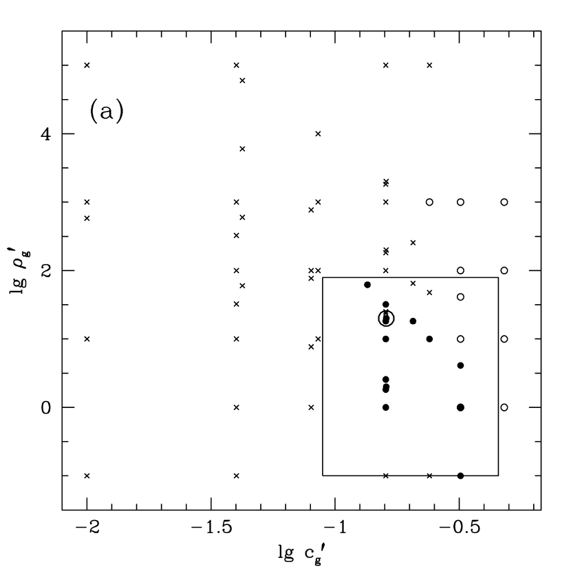
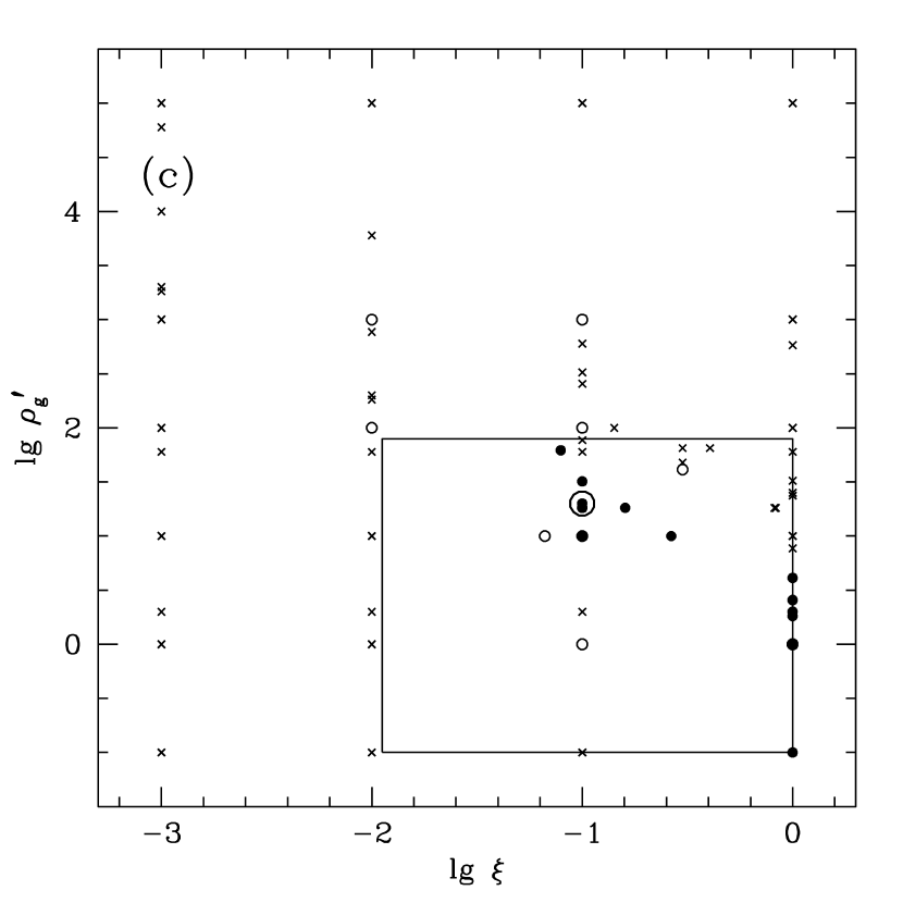
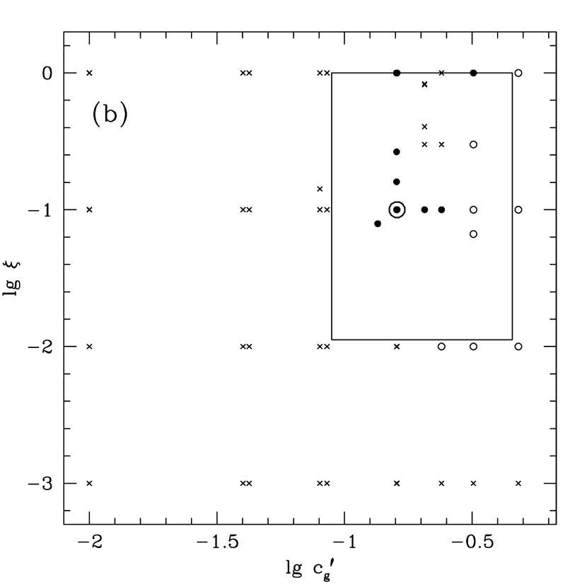
Figure 3.— Illustration of our best fitting model search algorithm for the Draco1 dataset (see Section 4), NFW halos and $\lambda=0.1$. Panels (a-c) show the projection of the models onto three orthogonal planes in the three-dimensional space of free model parameters $c_{g}^{\prime}$, $\rho_{g,0}^{\prime}$, and $\xi$. Crosses mark models which have unphysical DM halos ($F<F_{\rm min}$). Small open circles correspond to physical ($F>F_{\rm min}$) models which have a bad $\chi^{2}$ fit between the modeled and observed surface brightness profiles ($\chi^{2}>2\chi_{\rm min}^{2}$, where $\chi_{\rm min}^{2}$ is the lowest $\chi^{2}$ value for all $\sim 700$ models). Solid circles show the location of models which both are physical ($F>F_{\rm min}$) and fit well the observed surface brightness profile ($\chi^{2}<2\chi_{\rm min}^{2}$). The large circle marks a physical model with the smallest $\chi^{2}$ value (for NFW halo and $\lambda=0.1$). Rectangular boxes delineate the area where good models are being looked for. Panel (d) shows the multivariate correlation between the three free parameters ($c_{g}^{\prime}$, $\rho_{g,0}^{\prime}$, and $\xi$) and the core line-of sight velocity dispersion $\sigma_{0}$ for models with $\chi^{2}<2\chi_{\rm min}^{2}$, which is used for searching for good models. Here crosses correspond to unphysical DM halos (with $F<F_{\rm min}$), whereas the solid circles mark physical halos ($F>F_{\rm min}$). Two horizontal dotted lines show the one-sigma errorbars for the observed $\sigma_{\rm obs,0}$ in Draco.

In this project we faced the formidable task of sampling 4-dimensional ($c_{g}^{\prime}$, $\rho_{g,0}^{\prime}$, $\xi$, and $\lambda$) initial parameter space in our numerical simulations (with an extra factor of 2 due to the two different types of DM halo profiles considered — NFW and Burkert). As we mentioned before, the requirement for gas to be colder than the virial temperature results in $0<c_{g}^{\prime}\lesssim 0.5$. Other obvious constraints are $0<\xi\leqslant 1$ and $0\leqslant\lambda<1$ (by definition). We had no other reasonably motivated constraints on the range of our free parameters.

Initially, we sampled a large range of the free parameter space by simulating a grid of models with $c_{g}^{\prime}=(0.01,0.04,0.16)$, $\rho_{g,0}^{\prime}=(0.1,10,10^{3},10^{5})$, $\xi=(0.001,0.01,0.1,1)$, and $\lambda=(0,0.1)$, which resulted in 192 models (both NFW and Burkert). We quickly realized that models with $c_{g}^{\prime}<0.04$ or $\rho_{g,0}^{\prime}>10^{3}$ can be safely ruled out as they all produced unacceptably large $\chi^{2}$ values (in other words — their surface brightness profiles were nothing like profiles of dSphs) and/or very low $F$ values being much smaller than $F_{\rm min}$ (meaning that the inferred DM halo parameters were improbable in the adopted $\Lambda$CDM cosmology) for our sample of galaxies.

Other important observations were: (1) the range for $c_{g}^{\prime}$ should be expanded up to $\sim 0.5$ to include warmer models (which we could not do for models with $\lambda=0$, as in most of such models the initial stellar half-mass radius becomes divergent for $c_{g}^{\prime}\gtrsim 0.2$); (2) in the range $0.04\dots 0.5$, the parameter $c_{g}^{\prime}$ should be better sampled (by a factor of two) ; (3) in the range $0.1\dots 10^{3}$, $\rho_{g,0}^{\prime}$ should also be better sampled (by a factor of two).

As a result, we ran 294 additional models, which also included a set of models with $\lambda=0.3$ (for such models we simulated only the cases with $c_{g}^{\prime}\geqslant 0.04$ and $\rho_{g,0}^{\prime}\leqslant 10^{3}$). Altogether, we had 486 models on a regularly spaced 4-dimensional grid.

The problem we faced at that point was that no realistic number of models on a regularly sampled 4-dimensional grid would be large enough to simultaneously satisfy all our three selection criteria (outlined in § 3.1). More specifically, despite the fact that for most of our galaxies a relatively large volume in the 4-dimensional parameter space would satisfy both the first and the third criteria from § 3.1, few (usually none) of the models from this volume would produce the core line-of-sight velocity dispersion $\sigma_{0}$ which would be consistent with observations within the measurement errors (our second criterion).

Fortunately, we found a solution for the above problem. We noticed that for the models which produce reasonably good $\chi^{2}$ fits (within a factor of two from the model with the lowest $\chi^{2}$ value), there is a good multivariate correlation (in logarithmic space) between $\sigma_{0}$ and the free parameters $c_{g}^{\prime}$, $\rho_{g,0}^{\prime}$, and $\xi$ for NFW models, and $\rho_{g,0}^{\prime}$ and $\xi$ for Burkert models (the parameter $\lambda$ is fixed).

Our strategy was then as follows. For each galaxy, each value of $\lambda$, and each type of DM profile (NFW or Burkert), we used a multivariate $\chi^{2}$ fitting to find coefficients for the $\sigma_{0}(c_{g}^{\prime},\rho_{g,0}^{\prime},\xi)$ correlation. (Only the models producing good surface brightness $\chi^{2}$ fits were used.) We used this correlation to randomly sample a plane $\sigma_{{\rm obs},0}=\sigma_{0}(c_{g}^{\prime},\rho_{g,0}^{\prime},\xi)$, with typically 10 additional models for each case. (Here $\sigma_{{\rm obs},0}$ is the observed core line-of-sight velocity dispersion, listed in Table 1.) The sampling was done within the three-dimensional rectangular volume corresponding to models which simultaneously satisfied our first and third criteria from § 3.1. As our method is not precise, not all additional models satisfied all the three criteria. Figure 3 illustrates our algorithm for the case of the Draco1 dataset (see Section 4), NFW halos, and the $\lambda=0.1$.

Overall, we simulated around 700 models. It took approximately 500 CPU-days to simulate all the models on McKenzie cluster at CITA composed of 256 dual Intel Xeon 2.4 GHz nodes networked with commodity gigabit ethernet. Each model was run on 4 CPUs, with many models running in parallel.

4. RESULTS FOR FOUR DWARF SPHEROIDAL GALAXIES

4.1. General Remarks

In Table 2 we show statistics on “good” models (which meet all three selection criteria from § 3.1) for five datasets considered in this paper — for the Draco (two datasets), Sculptor, Carina, and Fornax dSphs. Because of the small number of “good” models $N_{g}$, the not completely random nature of our best fitting models search algorithm, and some degree of noisiness in the results of our simulations, in this table we present three complimentary statistical measures for each parameter and for each dataset: the value for the “best” model (producing the smallest value of $\chi^{2}$ in surface brightness profile fitting), the mean value with the associated standard deviation, and the total range for all $N_{g}$ models. Most of the parameters are presented as their logarithms as their distribution is much less skewed in logarithmic space. For the same reason, instead of the redshift, $z$, of halo formation, we present statistics on the cosmic scale factor $a=1/(1+z)$.

We use the following definition of tidal radius $r_{\rm tid}$ (Hayashi et al., 2003):

$$\frac{M(r_{\rm tid})}{r_{\rm tid}^{3}}=\left[2-\frac{R}{M_{H}(R)}\frac{\partial M_{H}}{\partial R}\right]\frac{M_{H}(R)}{R^{3}}.$$ (20)

Here $M(r)$ and $M_{H}(R)$ are enclosed mass functions for the satellite and host galaxies. We assumed that Milky Way DM halo has NFW density profile with $M_{\rm vir}=1.5\times 10^{12}$ M_⊙ (corresponding to $R_{\rm vir}=298$ kpc). From equation (14) of Sternberg et al. (2002), the concentration of the Milky Way halo is $c=13.2$. The tidal radius was calculated for the current distances $D$ (listed in Table 1) of the dSphs from the Galactic center.

To calculate the temperature $T$ of the gas, we assumed that the mean molecular weight is $\mu=1.218m_{p}$, which is appropriate for neutral gas of primordial composition. (Here $m_{p}$ is the mass of the proton.) If gas is ionized, the temperature would be a factor of 2 smaller.

In the next four sections we also present surface density $\Sigma(r)$ and line-of-sight velocity dispersion $\sigma(r)$ profiles for our best fitting models for each dataset (Figures 4-8). Only those parts of the profiles which have a standard deviation (estimated from the last $N_{S}$ snapshots for a given radial bin) smaller than 0.2 dex for $\Sigma(r)$ and 1 km s^-1 for $\sigma(r)$ are shown. For comparison, we show the surface density profiles for the best fitting theoretical King (1966) models (dashed lines).

4.2. Draco

Figure 4.— Best fitting models for the Draco1 dataset. (a) Surface density profiles. The observed profile is shown as solid circles with errorbars. The solid line corresponds to the best fitting model (with the lowest $\chi^{\prime 2}$). The dashed line shows the best fitting theoretical King model profile. (b) Line-of-sight velocity dispersion profiles for all 11 “good” models from Table 2. The thick line corresponds to the model with the lowest $\chi^{\prime 2}$.

Figure 5.— Best fitting models for the Draco2 dataset. (a) Surface density profiles. The observed profile is shown as solid circles with errorbars. The solid line corresponds to the best fitting model (with the lowest $\chi^{\prime 2}$). The dashed line shows the best fitting theoretical King model profile. (b) Line-of-sight velocity dispersion profiles for all 13 “good” models from Table 2. The thick line corresponds to the model with the lowest $\chi^{\prime 2}$.

Draco is probably the best candidate for having an extended DM halo among Galactic dSph satellites. Odenkirchen et al. (2001) used deep multicolor photometry covering 27 square degrees around the center of this galaxy to show that Draco has a very regular structure (with no signs of tidal interaction with the Milky Way gravitational field) out to the radius where its surface brightness falls to 0.003 of the central value. Their results suggested that there is much more DM in the outskirts of Draco than in its center.

More recently, Wilkinson et al. (2004) presented a new star number count profile for Draco. The new profile appears to be even more shallow in the outskirts of the galaxy than the profile of Odenkirchen et al. (2001), though the two profiles are marginally consistent. Wilkinson et al. (2004) also published a line-of-sight velocity dispersion profile for Draco, which is roughly isothermal, with the exception of the last radial bin where the stars are marginally colder than the rest of the galaxy.

We use star count profiles from both Odenkirchen et al. (2001, their sample S2, which has a lower estimated foreground/background contamination level than their sample S1) and Wilkinson et al. (2004) in our analysis, which we designate Draco1 and Draco2, respectively. We found 11 and 13, respectively, “good” models for these two datasets (see Table 2). In both cases, our models produce much better $\chi^{2}$ surface brightness fits than best fitting King models ($\chi^{\prime 2}\equiv\chi^{2}/\chi^{2}_{\rm King}\sim 0.6$). As can be seen in Figures 4a and 5a, the only statistically significant difference between our best fitting models and King models is in the outer parts of the galaxy. In the Draco outskirts, the King models exhibit a sharp cutoff due to the external tidal field, whereas our models have a relatively shallow power-law profile, which is completely consistent with the observed profiles. Virtually all of our best fitting models have non-zero value for the star formation lower density cutoff $\lambda$, which results in the outskirts of the galaxy appearing to be dynamically colder in the model $\sigma(r)$ profile, consistent with the observations of Wilkinson et al. (2004). As we showed in § 2.5, the total velocity dispersion in our models with $\lambda>0$ does not decrease with radius, with the observed decline of the line-of-sight velocity dispersion being due to significant radial anisotropy exhibited by our models outside the initial (non-equilibrium) stellar radius $x_{\lambda}$ (see Figure 2b).

As can be seen from Table 2, the best fitting models for Draco have a large range of DM halo virial masses $\sim 10^{8}-10^{10}$ M_⊙. These masses are all significantly larger than conventional estimates of $\sim 2\times 10^{7}$ M_⊙ (Mateo, 1998) which are based on the assumption that “mass follows light”. The total range for halo formation redshifts is $\sim 1.3-10$, corresponding to a galaxy age $\sim 9-13$ Gyr, which is consistent with the estimated age of the oldest Draco stars of $10-14$ Gyr (Mateo, 1998).

It is interesting to note that a comparable number of both NFW and Burkert models provided good fits to the observed Draco profiles. (Out of 24 “good” models for Draco1 and Draco2 datasets, there are 16 NFW and 8 Burkert profiles.) Even more interesting is the fact that for 16 “good” NFW models $\nu_{c}\simeq-1.21\pm 0.44$, whereas for 8 Burkert models $\nu_{c}\simeq 1.16\pm 0.31$. It appears that the Draco galaxy is best described by models with either underdense NFW or overdense Burkert DM halos, which is consistent with Draco having a DM halo with an intermediate value of its central density slope of $\gamma\sim-0.5$.

The predictions of our models for the initial gas state in Draco appear to be sensible, with the temperature of $\sim 20,000$ K ($\sim 10,000$ K if the gas was ionized) and the central number density of $\sim 10$ cm^-3. The lowest density for star-forming gas is $\sim 1-2$ cm^-3. After the starburst, the stellar cluster in all “good” models expanded by a very modest factor of $\sigma_{\rm ini,0}/\sigma_{0}\sim 1.2$.

Overall, our simple model of single-burst star formation from isothermal gas in an extended DM halo appears to provide an adequate description of the Draco dSph.

4.3. Sculptor

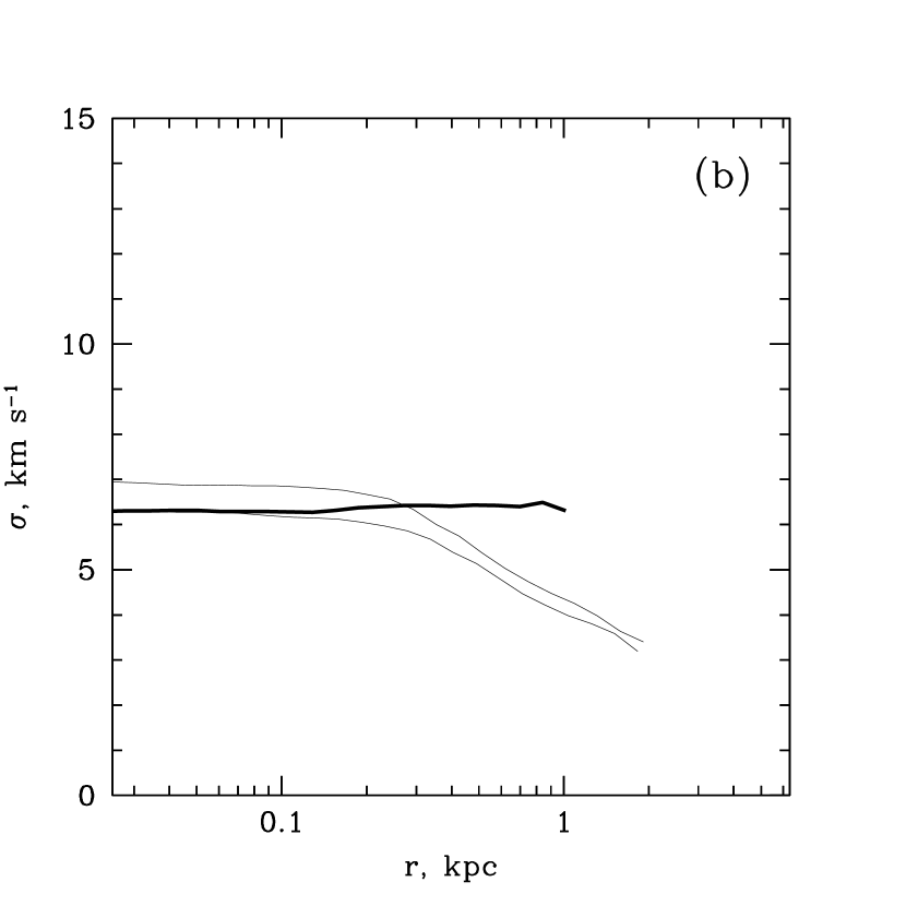
Figure 6.— Best fitting models for Sculptor. (a) Surface density profiles. The observed profile is shown as solid circles with errorbars. The solid line corresponds to the best fitting model (with the lowest $\chi^{\prime 2}$). The dashed line shows the best fitting theoretical King model profile. (b) Line-of-sight velocity dispersion profiles for all 3 “good” models from Table 2. The thick line corresponds to the model with the lowest $\chi^{\prime 2}$.

For Sculptor (and also for Carina and Fornax) we used star count profiles from Walcher et al. (2003). The authors use single-color photometry to identify stars belonging to these galaxies. As a result, the star count profiles for these three dSphs are of much lower quality than the Draco data of Odenkirchen et al. (2001), who employed a multicolor mask filtering technique to improve the sensitivity to Draco stars by a factor of $\sim 30$. One has to keep in mind that simple single-color techniques [such as used by Walcher et al. (2003)] can produce very unreliable results at surface brightness levels below the foreground/background contamination level. For example, according to the single-color photometry of Irwin & Hatzidimitriou (1995), Draco has a flat surface brightness profile beyond 20 arcmin from the galactic center (which was interpreted as a halo of unbound stars). In contrast, much higher sensitivity multicolor observations of Odenkirchen et al. (2001) failed to find any evidence for such a halo.

In all the three galaxies (Sculptor, Carina, and Fornax) some of the radial bins in their outskirts have negative surface brightness values (Walcher et al. 2003; this is an artifact of background subtraction procedure). In the case of Sculptor, even the upper one-sigma errorbar is negative for the bin at $r\sim 2$ kpc. As a result, we could not show this bin value in Figure 6a. Our $\chi^{2}$ fitting is not affected by the negative values of surface brightness, as we perform the cross-correlation in linear space.

With all the above caveats in mind, our model appears to do a reasonably good job in describing the properties of Sculptor. Formally, we have only one “good” model for this galaxy, with $\chi^{\prime 2}=0.94$ (see Table 2). On the other hand, we have a large number of models with $\chi^{2}$ slightly worse than for the best fitting King model: 3 models with $\chi^{\prime 2}<1.1$, and 11 models with $\chi^{\prime 2}<1.5$. As will be seen in § 4.5, this is very different from the case of Fornax, where the best model has $\chi^{\prime 2}\sim 1.1$, and the second-to-best has $\chi^{\prime 2}\sim 1.9$.

Analysis of Figure 6a shows that our best fitting model improves upon theoretical King model by having a less steep outer surface brightness profile, which is the same situation as with Draco (see § 4.2). One cannot have a much better fit with a smooth function due to the fact that the data are very noisy in the outer parts of the galaxy, with the star counts of $-0.31\pm 0.02$ arcmin^-2 at $r\sim 2.1$ kpc and $0.09\pm 0.02$ in the next radial bin at $r\sim 2.6$ kpc.

Properties of three models with $\chi^{\prime 2}<1.1$ are summarized in Table 2. With such small statistics it is hard to draw any conclusions on the range of model parameters, but it appears that all the main parameters for Sculptor are comparable to those for Draco. Most importantly, the virial mass for the DM halo is required to be $\gtrsim 3\times 10^{8}$ M_⊙, which is much larger than the $6.4\times 10^{6}$ M_⊙ estimate of Mateo (1998) based on the $\Upsilon=constant$ assumption. (Interestingly, the two H i clouds observed in the vicinity of Sculptor, which were argued by Bouchard, Carignan, & Mashchenko (2003) to be a part of ISM of this galaxy, are located in projection well within the inferred large tidal radius of $\sim 7.5$ kpc, corresponding to $\sim 5.5$ angular degrees at the distance $D=79$ kpc). The notable difference from the Draco case is a factor of two lower temperature, which is of order of 10,000 K for neutral gas (see Table 2).

4.4. Carina

Figure 7.— Best fitting models for Carina. (a) Surface density profiles. The observed profile is shown as solid circles with errorbars. The solid line corresponds to the best fitting model (with the lowest $\chi^{\prime 2}$). The dashed line shows the best fitting theoretical King model profile. (b) Line-of-sight velocity dispersion profiles for all 6 “good” models from Table 2. The thick line corresponds to the model with the lowest $\chi^{\prime 2}$.

Similarly to Sculptor, the surface brightness profile for Carina is very noisy at $\Sigma\lesssim 0.01\Sigma_{0}$ (see Figures 6a and 7a), with $\Sigma$ being negative at $r\sim 1.3$ kpc. We found 6 “good” models for Carina, with $\chi^{\prime 2}=0.84$ for the best fitting model (Table 2). As in the cases of Draco and Sculptor, the surface brightness profiles of our Carina models are identical to the best fitting theoretical King model in the inner part of the galaxy, and become less steep in its outskirts.

Unlike Draco and Sculptor, all “good” Carina models have Burkert DM density profile. All virial masses are larger than $\sim 3\times 10^{8}$ M_⊙, and are typically around $10^{9}$ M_⊙. [Mateo (1998) gives $1.3\times 10^{7}$ M_⊙.] Such masses are large enough to keep fully photoionized ISM gravitationally bound, which is a prerequisite for the radiation harassment picture proposed by Mashchenko et al. (2004) to explain the complex star formation history of this dwarf (Mateo, 1998). All 6 models have a halo formation redshift of $\sim 5.7$ (lookback time 12.6 Gyr), which is consistent with the $\sim 10-14$ Gyr age of the oldest stars in this galaxy (Mateo, 1998). The rest of the model parameters are comparable to the Draco and Sculptor cases.

4.5. Fornax

Figure 8.— Best fitting model for Fornax. (a) Surface density profiles. The observed profile is shown as solid circles with errorbars. The solid line corresponds to the best fitting model (with the lowest $\chi^{\prime 2}$). The dashed line shows the best fitting theoretical King model profile. (b) Line-of-sight velocity dispersion profile for the model with the lowest $\chi^{\prime 2}$.

Fornax is the only galaxy in our sample with not a single model which would simultaneously meet all the three selection criteria from § 3.1. In Table 2 we list parameters for the only model which has a comparable $\chi^{2}$ to the best fitting King model: $\chi^{\prime 2}=1.09$. The second-to-best model has $\chi^{\prime 2}=1.9$.

One could try to argue that the failure to find a model with $\chi^{\prime 2}<1$ is due to the fact that the King model already provides an almost perfect fit to the data (see Figure 8a). It is conceivable that with unlimited computing resources we would be able to fine-tune our initial parameters to find a model which would fit the observed surface brightness profile slightly better than the King model. However, King-like profiles are not natural for our models (which typically have less steep outer density profiles), and it would be very unlikely that it is a mere accident that Fornax happened to have an almost perfect King profile. The tidal stripping process, on the other hand, drives naturally an isothermal stellar system toward a King-like state, which makes it a more attractive explanation for the Fornax observed properties.

The inferred parameters for our best fitting model (Table 2) make even more questionable the applicability of our model to Fornax. In particular, the inferred central gas density $\rho_{g,0}\sim 0.9$ cm^-3 is much lower than for the other three dSphs. Furthermore, all models with $\chi^{\prime 2}\lesssim 3$ have $\lambda=0$. It seems unphysical for star formation to take place with almost 100% efficiency (see Table 2) at densities $\ll 1$ cm^-3.

All of the above leads us to conclude that our model (at least in its present, simplest form) is not applicable to the Fornax dSph. It remains to be seen if some other non-tidal mechanism could produce naturally a King-like surface brightness profile in a dSph. For now, Fornax being a tidally limited system seems to be the most likely explanation. It is interesting to note that even in the tidally limited scenario, Fornax appears to have a quite large mass, with the “mass follows light” estimate of $6.8\times 10^{7}$ M_⊙ (Mateo, 1998), and potentially even larger value if Fornax is more DM dominated in its outskirts.

5. DISCUSSION

The observational data on three galaxies (Draco, Sculptor, and Carina) out of four dSphs studied in this paper appear to be consistent with our simple model of star formation in extended DM halos, and as a consequence are consistent with them having very massive DM halos. The galaxy with the best quality star count profiles (Draco) is also the one which makes the most convincing case for having an extended halo — both in the analysis of Odenkirchen et al. (2001) who showed that the outer stellar isophotes for Draco are not tidally distorted, and in the analysis carried out in this paper.

The data for Fornax appear not to be consistent with the predictions of our model. The surface brightness profile for this galaxy is almost perfectly described by a theoretical King model, which was derived for an isothermal system exposed to external tidal field. This type of profile does not come naturally in our model. In addition, the best fitting model for Fornax predicts that the star formation in this dwarf should have taken place at unphysically low densities of $\ll 1$ cm^-3. The results of our simulations are thus suggestive of the cutoff in the outer surface brightness profile of Fornax being caused by the tidal field of the Milky Way.

The situation is significantly different with the three other dSphs we studied in this paper (Draco, Sculptor, and Carina), which appear to have extended DM halos. This difference can be explained if (1) the orbit of Fornax has a significantly smaller pericenter distance than the orbits of the other three galaxies [but this seems to be inconsistent with the available proper motion measurements (Dinescu et al., 2004), which imply that Fornax is on a low eccentricity orbit and is currently near its pericenter], and/or (2) the average DM density within the stellar extent of Fornax (radius of $\sim 4$ kpc) is significantly smaller than the average DM density within the same radius of the three other dSphs. (The latter would be the case if Fornax was formed more recently than the three other galaxies.)

The conclusion we reach here is quite contrary to the conventional argument that the presence of “extratidal” stars (those which populate the outer halo of the dwarf galaxy beyond the tidal radius of the best-fitting King model) around Milky Way satellites is a good evidence for the dwarf galaxy to have undergone a tidal disruption process, with the observed “extratidal” stars being part of the halo of tidally stripped stars. In our model, star formation in extended DM halos naturally produces surface brightness profiles which are identical to King profiles out to a few core radii, and are less steep in the outer parts of the galaxy. The example of Fornax suggests that actually the absence of “extratidal” halo, with the galactic surface brightness profile being described almost perfectly by theoretical King profile, could be an evidence for the galaxy to be observed all the way to its tidal radius. In such tidally limited systems a small number of stars do have to populate an extratidal halo, forming leading and trailing tidal tails, but for stable satellite galaxies the surface brightness of such tails can be very low (especially if dSphs have more DM in their outskirts than at the center, which appears to be the case for Draco), potentially below the sensitivity of existing observations. The systems where tidal tails have been reliably detected (such as Sagittarius dSph and Palomar 5) are at the last stage of being tidally disrupted, which cannot be the case for most Galactic dSphs. We argue that to rule out our alternative, non-tidal explanation for the presence of “extratidal” stars around some Galactic dSphs, unambiguous observational evidence for these stars forming leading and trailing tidal tails has to be obtained.

Recent observations suggest that in some Galactic dSphs (Draco, Ursa Minor, and Sextans) the very outskirts of the galaxies have lower values of line-of-sight velocity dispersion than the bulk of the galaxy (Wilkinson et al., 2004; Kleyna et al., 2004). In our models, this is the case for all models with sufficiently large lower density cutoffs for star formation: $\lambda\gtrsim 0.1$ (see Figures 4b-6b). For such models, we observe the line-of-sight velocity dispersion to decline by a factor of two in the outer parts of the galaxy, which is caused by strong radial anisotropy of stars which were born within the initial stellar cluster radius $r_{\lambda}$ and then later populated the $r>r_{\lambda}$ parts of the galaxy.

The Fornax (Mateo, 1997), Draco (Wilkinson et al., 2004), and Sextans (Kleyna et al., 2004) observations suggest that these galaxies are kinematically colder at the center than in the intermediate regions. Such behavior cannot be explained in terms of our single star burst model. Many dSphs however have complex ancient ($\gtrsim 10$ Gyr old) star formation histories, with slightly younger and/or more metal rich stars being more concentrated toward the center (Harbeck et al., 2001; Tolstoy et al., 2004). A natural extension of our model then would be to assume that a fraction of gas, which was somewhat metal-enriched and expelled to large radii during the first star burst, was later reaccreted, leading to the second episode of star formation. The reaccretion of the gas and the second star burst can be delayed by up to a few Gyrs by supernovae type Ia occurring in the original stellar population (Burkert & Ruiz-Lapuente, 1997). Let us consider the simplified case of negligible self-gravity of gas [$m^{\prime}_{g}\ll M^{\prime}(x)$ in eq. (6)], with the most of the gas being within the scaling radius $r_{s}$ of the DM halo [so that $M^{\prime}(x)\propto x^{\alpha}$, where $\alpha=2$ for NFW halos, and 3 for Burkert halos]. With the above simplifying assumptions, equation (6) can be rewritten as

$$\frac{d\rho^{\prime}_{g}}{dx}\propto-\frac{\rho^{\prime}_{g}}{c_{g}^{\prime 2}}x^{\alpha-2}.$$ (21)

The solution for this equation is

$$\rho_{g}^{\prime}(x)=\rho^{\prime}_{g,0}\exp\left[-\frac{Bx^{\alpha-1}}{c_{g}^{\prime 2}}\right],$$ (22)

where $B$ is some positive constant. For the case of $\alpha>1$, the total gas mass is

$$m^{\prime}_{g}\propto\rho^{\prime}_{g,0}c_{g}^{\prime 6/(\alpha-1)}.$$ (23)

We assume, that a star burst in a slowly cooling and contracting gas cloud will take place when the central gas density $\rho^{\prime}_{g,0}$ reaches a certain critical value, which is the same for the original star burst (the total gas mass $m^{\prime}_{g,1}$) and the subsequent star burst (the total gas mass $m^{\prime}_{g,2}$). Using equation (23), we can then relate the gas parameters for the two star bursts through

$$\frac{c_{g,2}^{\prime}}{c_{g,1}^{\prime}}=\left(\frac{m^{\prime}_{g,2}}{m^{\prime}_{g,1}}\right)^{(\alpha-1)/6}.$$ (24)

Here $c_{g,1}^{\prime}$ and $c_{g,2}^{\prime}$ are the sound speed in the gas in the first and second star bursts. The exponent in equation (24) is positive for both Burkert and NFW halos (the exponent values are $1/3$ and $1/6$, respectively). Due to gas consumption by star formation, and potentially some additional gas losses into intergalactic space, the total gas mass in the second star burst is smaller than in the original star burst: $m^{\prime}_{g,2}<m^{\prime}_{g,1}$. From equation (24), this results in the sound speed (and hence the temperature) of the gas in the second star burst being lower than in the first one: $c_{g,2}^{\prime}<c_{g,1}^{\prime}$. Both lower temperature and lower total gas mass will also result in the gas cloud being more compact in the second star burst. As a result, a kinematically colder stellar core, slightly younger and slightly more metal rich than the bulk of the galaxy, could be formed. A multiple star bursts scenario can explain the radial population gradients observed in many Local Group dSphs (Harbeck et al., 2001), and possibly the kink observed in the surface brightness profile of Draco at the radius of $\sim 25$ arcmin (Wilkinson et al., 2004). [Note that no kink is observed in the Draco profile of Odenkirchen et al. (2001).]

For the three galaxies, which appear to be consistent with our model (Draco, Sculptor, and Carina), the values of the inferred model parameters presented in Table 2 do not differ much from one galaxy to another. The “good” models for these galaxies have a shallow inner DM density profile (with the slope $\gamma\sim-0.5\dots 0$), which is consistent with the observations of dwarf spiral galaxies (Burkert, 1995), dwarf irregular galaxies (Côté, Carignan, & Freeman, 2000), and low surface brightness galaxies (e.g. Marchesini et al., 2002). The typical virial masses for the DM halos are of order of $\sim 10^{9}$ M_⊙, with the total range spanning from $9\times 10^{7}-2\times 10^{10}$ M_⊙. These masses are much larger than those obtained under assumption of constant mass-to-light ratio, and are consistent with the idea that dSphs represent the largest subhalos expected to populate the Milky Way halo in cosmological $\Lambda$CDM simulations (Stoehr et al., 2002; Hayashi et al., 2003), alleviating the “missing satellites” problem of such cosmologies (Moore et al., 1999). The inferred formation redshifts for these galaxies are $\sim 2-6$ (lookback time $\sim 10-13$ Gyr), which is consistent with the age of the oldest stars in these galaxies (Mateo, 1998). The virial radii for the DM halos at the time of their formation range from $1.4-30$ kpc, whereas the tidal radii at their current distance from the Milky Way center are $5-32$ kpc (typically $\sim 10$ kpc, which would correspond to $\sim 6$ angular degrees in the sky for these three dSphs). Both virial and tidal radii are significantly larger than the observed extent of these galaxies.

The star forming gas in the “good” models has a temperature of $\sim 10,000-20,000$ K if it is neutral ($\sim 5000-10,000$ K if it is ionized), a central density of $\sim 10$ cm^-3, and a central pressure of $\sim 10^{5}$ K cm^-3. The temperature of the gas is a factor of $\sim 2.5$ lower than the virial temperature of the DM halo (defined in § 2.4), suggesting that the gas accreted by the DM halo experienced only modest level of radiative cooling globally prior to the starburst. The lower density cutoff for star formation is of order of $\sim 1$ cm^-3. The inferred star formation efficiency in the star-forming central part of ISM is $\sim 10$%.

We argue that our results are not very sensitive to the model assumption that the DM potential is static. During the formation of a dwarf spheroidal galaxy, gradual collapse of the gas cloud due to radiative cooling and gravitational instability will lead to the adiabatic contraction of the DM halo in the central region of the galaxy, where the enclosed gas mass becomes larger than that of DM. Proper modeling of this process requires adding many physical processes (live DM halo, non-equilibrium chemistry, radiative heating and cooling) with many associated free parameters, which is beyond the scope of this paper. Instead, we argue that our main results should not be significantly affected by the above effect by noting that (1) in our best fitting models, gas does not significantly dominate DM at the center of the galaxy (with the maximum ratio of the enclosed gas mass to that of DM of 10 for the Sculptor best fitting model; in case of the Draco1 dataset, this ratio is less than $1/3$ at any radius), and (2) the initial adiabatic contraction of the DM halo will be compensated by the adiabatic expansion caused by the removal of $\sim 90$% of baryons from the central part of the galaxy by stellar feedback mechanisms after the starburst.

Another potential pitfall is our assumption that the tidal field of Milky Way played no role in shaping the stellar outskirts of the dSphs we studied. Judging from the data presented in Table 2, this assumption appears to be justified. In particular, the inferred tidal radii are significantly larger than the observed extent of these dwarfs (by a factor of $>2$). We do not expect many dSph stars to be tidally stripped under these circumstances. More accurate analysis of this effect is complicated as it would involve high resolution $N$-body simulations of a two-component (DM $+$ stars) dwarf satellite in the potential of the host galaxy with some prescription for dynamical friction to describe the orbital decay, and with many poorly known orbital and Milky Way halo parameters. This task is beyond the scope of our paper, where our main goal is to sample well the initial model parameter space, with the only practical way of achieving this being in keeping the number of free parameters as small as possible.

The selective nature of the tidal disruption of satellites in the halo of the host galaxy could make our method of finding the most likely DM halo progenitors for Galactic dSphs (§ 3.3) invalid. However, this effect would be important only if the DM halos in our best fitting models were relatively easy to disrupt over the Hubble time in the tidal field of Milky Way. In the case of the Draco1 dataset, the best fitting model has an NFW DM density profile and the inferred tidal radius of $\sim 4.4r_{s}$ (Table 2). Numerical simulations of Hayashi et al. (2003) demonstrated that NFW subhalos orbiting in the host halo potential stay relatively intact after $\gtrsim 10$ orbits if $r_{\rm tid}>2r_{s}$. In this respect, the Draco1 model appears to be stable. In the three remaining datasets (Draco2, Sculptor, and Carina; we exclude Fornax from this analysis), the DM halos of the best fitting models have Burkert profiles, with the tidal radii $r_{\rm tid}>10r_{s}$. Burkert satellites are easier to disrupt tidally than NFW satellites, as their binding radius is $\sim 2.1$ times larger (Mashchenko & Sills, 2005b). Nevertheless, the large inferred value of the tidal radius ($>10r_{s}$) makes it very unlikely that the Burkert DM halos corresponding to our best fitting models would be completely destroyed by the tidal field of Milky Way in a Hubble time.

We believe that our model is consistent with the observed metallicities of Galactic dSphs. As can be seen in Fig. 7 of Mateo (1998) and Fig. 1 of Tamura et al. (2001), the low-luminosity objects we are interested in show a relatively large spread in metallicity (with a typical value of [Fe/H]$\sim-1.8$) and no statistically significant correlation between metallicity and luminosity or (conventionally derived) virial mass. The only exception among the Galactic dSphs is Fornax, which is both the brightest and the most metal-rich ([Fe/H]$\sim-1.3$, Mateo 1998). As we discussed above, Fornax is not well described by our model. If we relax the single starburst assumption, more massive galaxies can become more metal-rich over time, as they have deeper gravitational potential wells and larger tidal radii, enabling them to reaccrete more metal-enriched gas expelled in the previous episode of star formation. Our model is consistent with the data if the Galactic dSphs were formed from a pre-enriched intergalactic medium, with [Fe/H]$\sim-2$.

6. CONCLUSIONS

Our simple model of stars forming in an extended DM halo from isothermal gas, and later dynamically relaxing after expelling the leftover gas, is consistent with the observed properties of three out of four dSphs studied in this paper.

The results of our simulations suggest that there is an alternative, non-tidal explanation for the observed presence of halos of “extratidal” stars around some Galactic dSphs. In our model, such halos are formed when a freshly formed stellar cluster is relaxed dynamically inside the extended DM halo.

The virial masses of DM halos, inferred from fitting our models to the three dSphs (Draco, Sculptor, and Carina), are in the right range ($\sim 10^{9}$ M_⊙) to give support to the idea that the Galactic dSphs represent the most massive subhalos predicted to orbit in the Milky Way halo by cosmological $N$-body $\Lambda$CDM simulations, alleviating in this way the “missing satellites” problem. The masses are also large enough to keep a fully ionized ISM gravitationally bound, which is an essential ingredient of some models (Burkert & Ruiz-Lapuente, 1997; Mashchenko et al., 2004) proposed to explain the complex star formation history of some Galactic dSphs.

Table 2Results of simulations

Parameter	Unit	Statistics	Draco1	Draco2	Sculptor	Carina	Fornax
$N_{g}$		$\cdots$	11	13	3	6	1
$\chi^{\prime 2}$		best	$0.67$	$0.58$	$0.94$	$0.84$	$1.09$
		mean	$0.78\pm 0.11$	$0.76\pm 0.14$	$1.03\pm 0.08$	$0.93\pm 0.06$	$\cdots$
		range	$0.67\dots 0.97$	$0.58\dots 1.00$	$0.94\dots 1.09$	$0.84\dots 1.00$	$\cdots$
$\lg F^{\prime}$		best	$0.70$	$1.44$	$1.89$	$1.91$	$1.30$
		mean	$0.70\pm 0.34$	$1.27\pm 0.69$	$0.79\pm 0.95$	$1.18\pm 0.74$	$\cdots$
		range	$0.02\dots 1.31$	$0.09\dots 2.21$	$0.12\dots 1.89$	$0.05\dots 2.07$	$\cdots$
$\gamma$		best	$-1.00$	$0.00$	$0.00$	$0.00$	$0.00$
		mean	$-0.82\pm 0.40$	$-0.54\pm 0.52$	$-0.67\pm 0.58$	$0.00\pm 0.00$	$\cdots$
		range	$-1.00\dots 0.00$	$-1.00\dots 0.00$	$-1.00\dots 0.00$	$0.00\dots 0.00$	$\cdots$
$\lg c_{g}^{\prime}$		best	$-0.79$	$-0.62$	$-0.80$	$-0.80$	$-0.80$
		mean	$-0.79\pm 0.04$	$-0.66\pm 0.18$	$-0.72\pm 0.06$	$-1.05\pm 0.23$	$\cdots$
		range	$-0.87\dots-0.69$	$-1.10\dots-0.49$	$-0.80\dots-0.69$	$-1.40\dots-0.80$	$\cdots$
$\lg\rho_{g,0}^{\prime}$		best	$1.30$	$0.48$	$1.00$	$0.00$	$0.00$
		mean	$0.83\pm 0.65$	$0.66\pm 0.68$	$1.36\pm 0.42$	$-0.12\pm 0.44$	$\cdots$
		range	$0.00\dots 1.79$	$-1.00\dots 1.51$	$1.00\dots 1.81$	$-1.00\dots 0.14$	$\cdots$
$\lg\xi$		best	$-1.00$	$-1.29$	$-0.63$	$-1.00$	$-0.15$
		mean	$-0.66\pm 0.45$	$-0.95\pm 0.25$	$-0.37\pm 0.28$	$-0.83\pm 0.41$	$\cdots$
		range	$-1.10\dots 0.00$	$-1.29\dots-0.41$	$-0.63\dots-0.08$	$-1.00\dots 0.00$	$\cdots$
$\lambda$		best	$0.10$	$0.10$	$0.00$	$0.10$	$0.00$
		mean	$0.14\pm 0.08$	$0.15\pm 0.11$	$0.07\pm 0.06$	$0.08\pm 0.12$	$\cdots$
		range	$0.10\dots 0.30$	$0.00\dots 0.30$	$0.00\dots 0.10$	$0.00\dots 0.30$	$\cdots$
$\lg M_{s}$	M⊙	best	$9.75$	$8.48$	$8.59$	$8.59$	$9.25$
		mean	$9.47\pm 0.33$	$8.86\pm 0.70$	$8.86\pm 0.26$	$9.26\pm 0.65$	$\cdots$
		range	$8.88\dots 10.05$	$7.98\dots 9.96$	$8.59\dots 9.12$	$8.49\dots 10.26$	$\cdots$
$\lg r_{s}$	kpc	best	$0.54$	$-0.30$	$-0.13$	$-0.12$	$0.27$
		mean	$0.41\pm 0.27$	$0.02\pm 0.42$	$0.23\pm 0.32$	$0.14\pm 0.23$	$\cdots$
		range	$-0.10\dots 0.74$	$-0.56\dots 0.59$	$-0.13\dots 0.47$	$-0.12\dots 0.49$	$\cdots$
$\lg M_{\rm vir}$	M⊙	best	$9.79$	$8.45$	$8.54$	$8.55$	$9.27$
		mean	$9.49\pm 0.34$	$8.86\pm 0.72$	$8.84\pm 0.28$	$9.23\pm 0.66$	$\cdots$
		range	$8.84\dots 10.06$	$7.93\dots 9.95$	$8.54\dots 9.11$	$8.46\dots 10.24$	$\cdots$
$a$		best	$0.35$	$0.10$	$0.14$	$0.14$	$0.24$
		mean	$0.34\pm 0.11$	$0.22\pm 0.13$	$0.33\pm 0.17$	$0.15\pm 0.01$	$\cdots$
		range	$0.11\dots 0.42$	$0.09\dots 0.40$	$0.14\dots 0.43$	$0.14\dots 0.17$	$\cdots$
$\nu_{c}$		best	$-0.94$	$1.16$	$0.22$	$0.14$	$-0.56$
		mean	$-0.90\pm 1.05$	$-0.01\pm 1.23$	$-1.60\pm 1.58$	$0.30\pm 0.34$	$\cdots$
		range	$-1.68\dots 1.42$	$-1.60\dots 1.70$	$-2.52\dots 0.22$	$-0.22\dots 0.74$	$\cdots$
$\lg(\sigma_{\rm ini,0}/\sigma_{0})$		best	$0.09$	$0.11$	$0.08$	$0.07$	$0.02$
		mean	$0.08\pm 0.01$	$0.10\pm 0.02$	$0.09\pm 0.02$	$0.05\pm 0.02$	$\cdots$
		range	$0.06\dots 0.10$	$0.07\dots 0.14$	$0.08\dots 0.12$	$0.03\dots 0.08$	$\cdots$
$\lg T$	K	best	$4.43$	$4.35$	$3.93$	$3.93$	$4.18$
		mean	$4.28\pm 0.09$	$4.32\pm 0.10$	$3.98\pm 0.09$	$3.84\pm 0.08$	$\cdots$
		range	$4.12\dots 4.43$	$4.11\dots 4.48$	$3.93\dots 4.08$	$3.76\dots 3.93$	$\cdots$
$\lg\rho_{g,0}$	cm-3	best	$0.87$	$1.29$	$1.41$	$0.38$	$-0.16$
		mean	$0.50\pm 0.50$	$0.86\pm 0.34$	$0.94\pm 0.48$	$0.16\pm 0.46$	$\cdots$
		range	$-0.23\dots 1.04$	$0.10\dots 1.29$	$0.45\dots 1.41$	$-0.77\dots 0.38$	$\cdots$
$\lg P$	K cm-3	best	$5.30$	$5.63$	$5.35$	$4.31$	$4.03$
		mean	$4.77\pm 0.57$	$5.18\pm 0.36$	$4.92\pm 0.49$	$3.99\pm 0.48$	$\cdots$
		range	$3.89\dots 5.41$	$4.48\dots 5.69$	$4.39\dots 5.35$	$3.03\dots 4.31$	$\cdots$
$\rho_{\lambda}$	cm-3	best	$0.74$	$1.94$	$0.00$	$0.24$	$0.00$
		mean	$0.66\pm 0.54$	$1.16\pm 0.90$	$0.39\pm 0.46$	$0.08\pm 0.11$	$\cdots$
		range	$0.06\dots 1.72$	$0.00\dots 2.68$	$0.00\dots 0.90$	$0.00\dots 0.24$	$\cdots$
$\lg r_{\rm vir}$	kpc	best	$1.31$	$0.35$	$0.50$	$0.51$	$0.99$
		mean	$1.16\pm 0.31$	$0.73\pm 0.47$	$0.92\pm 0.37$	$0.78\pm 0.23$	$\cdots$
		range	$0.54\dots 1.47$	$0.14\dots 1.36$	$0.50\dots 1.17$	$0.51\dots 1.16$	$\cdots$
$\lg r_{\rm tid}$	kpc	best	$1.18$	$0.88$	$0.88$	$0.96$	$1.25$
		mean	$1.10\pm 0.07$	$0.95\pm 0.19$	$0.87\pm 0.04$	$1.18\pm 0.22$	$\cdots$
		range	$1.00\dots 1.24$	$0.71\dots 1.35$	$0.83\dots 0.90$	$0.91\dots 1.50$	$\cdots$

Note. — Here $\chi^{2}_{\rm King}$ is the $\chi^{2}$ value for the best fitting theoretical King model.

Note. — Here $N_{g}$ is the number of “good” models (satisfying all three selection creteria from § 3.1), $\chi^{\prime 2}\equiv\chi^{2}/\chi^{2}_{\rm King}$, $F^{\prime}\equiv F/F_{\rm min}$, $a=1/(1+z)$, $\rho_{g,0}$ is the central number density of gas, $P=\rho_{g,0}T$ is the central gas pressure, $\rho_{\lambda}=\rho_{g,0}\lambda$, $r_{\rm vir}$ is the halo virial radius at the formation epoch, and $r_{\rm tid}$ is the current tidal radius (see definition in text).

References

- Bode, Ostriker, & Turok (2001) Bode, P., Ostriker, J. P., & Turok, N. 2001, ApJ, 556, 93
- Bouchard, Carignan, & Mashchenko (2003) Bouchard, A., Carignan, C., & Mashchenko, S. 2003, AJ, 126, 1295
- Boylan-Kolchin, Ma, & Quataert (2004) Boylan-Kolchin, M., Ma, C., & Quataert, E. 2004, ApJ, 613, L37
- Bryan & Norman (1998) Bryan, G. L. & Norman, M. L. 1998, ApJ, 495, 80
- Bullock et al. (2001) Bullock, J. S., Kolatt, T. S., Sigad, Y., Somerville, R. S., Kravtsov, A. V., Klypin, A. A., Primack, J. R., & Dekel, A. 2001, MNRAS, 321, 559
- Burkert (1995) Burkert, A. 1995, ApJ, 447, L25
- Burkert & Ruiz-Lapuente (1997) Burkert, A. & Ruiz-Lapuente, P. 1997, ApJ, 480, 297
- Côté, Carignan, & Freeman (2000) Côté, S., Carignan, C., & Freeman, K. C. 2000, AJ, 120, 3027
- Dinescu et al. (2004) Dinescu, D. I., Keeney, B. A., Majewski, S. R., & Girard, T. M. 2004, AJ, 128, 687
- El-Zant, Shlosman, & Hoffman (2001) El-Zant, A., Shlosman, I., & Hoffman, Y. 2001, ApJ, 560, 636
- Harbeck et al. (2001) Harbeck, D., et al. 2001, AJ, 122, 3092
- Hayashi et al. (2003) Hayashi, E., Navarro, J. F., Taylor, J. E., Stadel, J., & Quinn, T. 2003, ApJ, 584, 541
- Haywood, Robin, & Creze (1997) Haywood, M., Robin, A. C., & Creze, M. 1997, A&A, 320, 428
- Irwin & Hatzidimitriou (1995) Irwin, M. & Hatzidimitriou, D. 1995, MNRAS, 277, 1354
- King (1966) King, I. R. 1966, AJ, 71, 64
- Kleyna et al. (2002) Kleyna, J., Wilkinson, M. I., Evans, N. W., Gilmore, G., & Frayn, C. 2002, MNRAS, 330, 792
- Kleyna et al. (2004) Kleyna, J. T., Wilkinson, M. I., Evans, N. W., & Gilmore, G. F. 2004, MNRAS, 354, L66
- Lake (1990) Lake, G. 1990, MNRAS, 244, 701
- Łokas (2002) Łokas, E. L. 2002, MNRAS, 333, 697
- Marchesini et al. (2002) Marchesini, D., D’Onghia, E., Chincarini, G., Firmani, C., Conconi, P., Molinari, E., & Zacchei, A. 2002, ApJ, 575, 801
- Mashchenko et al. (2004) Mashchenko, S., Carignan, C., & Bouchard, A. 2004, MNRAS, 352, 168
- Mashchenko & Sills (2005a) Mashchenko, S., & Sills, A. 2005a, ApJ, 619, 243
- Mashchenko & Sills (2005b) Mashchenko, S., & Sills, A. 2005b, ApJ, 619, 258
- Mateo (1997) Mateo, M. 1997, ASP Conf. Ser. 116: The Nature of Elliptical Galaxies, 259
- Mateo (1998) Mateo, M. L. 1998, ARA&A, 36, 435
- Mateo et al. (1998) Mateo, M., Olszewski, E. W., Vogt, S. S., & Keane, M. J. 1998, AJ, 116, 2315
- Moore et al. (1999) Moore, B., Ghigna, S., Governato, F., Lake, G., Quinn, T., Stadel, J., & Tozzi, P. 1999, ApJ, 524, L19
- Navarro et al. (1997) Navarro, J. F., Frenk, C. S., & White, S. D. M. 1997, ApJ, 490, 493
- Odenkirchen et al. (2001) Odenkirchen, M., et al. 2001, AJ, 122, 2538
- Sheth & Tormen (1999) Sheth, R. K. & Tormen, G. 1999, MNRAS, 308, 119
- Spergel et al. (2003) Spergel, D. N., et al. 2003, ApJS, 148, 175
- Springel et al. (2001) Springel, V., Yoshida, N., & White, S. D. M. 2001, New Astronomy, 6, 79
- Sternberg et al. (2002) Sternberg, A., McKee, C. F., & Wolfire, M. G. 2002, ApJS, 143, 419
- Stoehr et al. (2002) Stoehr F., White S. D. M., Tormen G., Springel V., 2002, MNRAS, 335, L84
- Sugiyama (1995) Sugiyama, N. 1995, ApJS, 100, 281
- Tamura et al. (2001) Tamura, N., Hirashita, H., & Takeuchi, T. T. 2001, ApJ, 552, L113
- Tasitsiomi (2003) Tasitsiomi, A. 2003, International Journal of Modern Physics D, 12, 1157 (preprint astro-ph/0205464)
- Tolstoy et al. (2004) Tolstoy, E. et al. 2004, ApJ, 617, L119
- van den Bergh (1999) van den Bergh, S. 1999, A&A Rev., 9, 273
- van den Bosch (2002) van den Bosch, F. C. 2002, MNRAS, 331, 98
- Walcher et al. (2003) Walcher, C. J., Fried, J. W., Burkert, A., & Klessen, R. S. 2003, A&A, 406, 847
- Wilkinson et al. (2002) Wilkinson, M. I., Kleyna, J., Evans, N. W., & Gilmore, G. 2002, MNRAS, 330, 778
- Wilkinson et al. (2004) Wilkinson, M. I., Kleyna, J. T., Evans, N. W., Gilmore, G. F., Irwin, M. J., & Grebel, E. K. 2004, ApJ, 611, L21
- Wolfire et al. (1995) Wolfire, M. G., Hollenbach, D., McKee, C. F., Tielens, A. G. G. M., & Bakes, E. L. O. 1995, ApJ, 443, 152