The stability of decelerating shocks revisited

Abstract

We present a new method for analyzing the global stability of the Sedov-von Neumann-Taylor self-similar solutions, describing the asymptotic behavior of spherical decelerating shock waves, expanding into ideal gas with density $\propto r^{-\omega}$. Our method allows to overcome the difficulties associated with the non-physical divergences of the solutions at the origin. We show that while the growth rates of global modes derived by previous analyses are accurate in the large wave number (small wavelength) limit, they do not correctly describe the small wave number behavior for small values of the adiabatic index $\gamma$. Our method furthermore allows to analyze the stability properties of the flow at early times, when the flow deviates significantly from the asymptotic self-similar behavior. We find that at this stage the perturbation growth rates are larger than those obtained for unstable asymptotic solutions at similar $[\gamma,\omega]$. Our results reduce the discrepancy that exists between theoretical predictions and experimental results.

1. Introduction

Shock waves play a crucial role in the evolution of a wide variety of astrophysical systems, such as the inter-stellar medium and the inter-galactic medium (for review see, e.g., Ostriker & McKee, 1988). The study of shock wave properties, and in particular of shock wave stability, is therefore relevant for a wide variety of astrophysical phenomena. The stability of planar steady shocks propagating into a uniform medium was demonstrated by Erpenbeck (1962). The stability of 1D shocks (with planar/cylindrical/spherical symmetry) propagating into both uniform and non-uniform media is commonly studied by analyzing self-similar shock solutions of the hydrodynamic equations, since self-similar solutions often allow analytic stability analysis and since in many cases self-similar solutions describe the asymptotic behavior of the flow (see, e.g., Zèldovich & Raizer, 1968).

Ryu & Vishniac (1987,1991) have studied the stability of the self-similar Sedov-von Neumann-Taylor solutions (Sedov, 1946; Von Neumann, 1947; Taylor, 1950), describing spherical shocks propagating into an ideal gas with a power-law density profile $\rho\propto r^{-\omega}$. They have studied both the ”local” and the ”global” stability of the solutions. The term ”local” stability analysis refers to approximate analysis of stability where flow properties are considered in a small region, where the spatial dependence of flow variables may be approximated as linear, and boundary conditions are neglected. The term ”global” stability refers to stability against perturbations with time independent spatial structure, which satisfy the flow boundary conditions. Analysis of stability against global modes of perturbation is often not useful for general time dependent flows, with time dependent spatial structure. Self-similar flows are an exception, since the spatial structure of such flows is time independent.

The amplitude of global modes of perturbations to the Sedov-von Neumann-Taylor solutions evolves with time as $t^{s}$. For expansion into uniform media $(\omega=0)$, the Sedov-von Neumann-Taylor shocks were found to be stable ($Re(s)<0$) for gas adiabatic index $\gamma>1.2$, and unstable (for a limited range of perturbation wave numbers) for $\gamma<1.2$, where the high density region behind the shock is sufficiently thin. Qualitatively similar results are obtained from the analysis of Ryu & Vishniac for $\omega$ values in the range $0<\omega<(7-\gamma)/(\gamma+1)$. For larger values of $\omega$, $(7-\gamma)/(\gamma+1)<\omega<3$, the solutions are ”hollow,” i.e., the density vanishes at some finite distance (behind the shock) away from the origin. The stability of ”hollow” solutions was examined by Goodman (1990), who found that the flow is unstable for large perturbation wave numbers $l$, with growth rate scaling as $l^{1/2}$. The local stability analysis of Ryu & Vishniac (1991) showed that the flow in the non-hollow solutions is convectively unstable (to local perturbations) in the range $3/\gamma<\omega<(7-\gamma)/(\gamma+1)$. The growth rate of the perturbation was studied numerically in one specific case ($\omega=0,\gamma=1.1,l=40$) by Mac Low & Norman (1993), and was found to be in good agreement with the prediction of Ryu & Vishniac.

Shock waves propagating into a steep density gradient $\omega>3$, are accelerating. The asymptotic behavior of such shocks is not described by the Sedov-von Neumann-Taylor solutions, but rather by a different family of self-similar solutions, derived by Waxman & Shvarts (1993). The stability of these solutions against global modes of perturbations was examined by Sari, Waxman & Shvarts (2000), who found that shock waves that accelerate at a rate faster than the critical rate $\ddot{R}R/\dot{R}^{2}=1$ are unstable for small and intermediate wave numbers, whereas shock waves accelerating at a slower rate, $\ddot{R}R/\dot{R}^{2}<1$, are stable for most wave numbers (here, $R(t)$ denotes the time dependent shock radius). They have further shown that perturbations of small wave numbers grow or decay monotonically, while perturbations of intermediate and high wave numbers oscillate in time.

The stability of spherical shocks propagating into a uniform medium was studied experimentally by Grun et al. (1991). For shocks propagating in Xenon, with adiabatic index $\gamma=1.06\pm 0.02$, perturbations growing as a power low of time were found, while in Nitrogen, $\gamma=1.3\pm 0.1$, shocks were found to be stable. These results are in qualitatively agreement with the predictions of Ryu & Vishniac (1987). However, the maximum growth rate measured was higher then the Ryu & Vishniac prediction by a factor of $\sim 1.7$, and was obtained at lower than predicted wave numbers, $l\sim 10$ instead of $l\sim 60$.

The cause for the discrepancy between the experimental results and the theoretical predictions is yet unknown. On the one hand, there are some preliminary claims that the the experimental results of Grun et al. (1991) are not accurate (Hansen et al., 2002). On the other hand, there are some difficulties in the theoretical analysis. Briefly, the Sedov-von Neumann-Taylor solutions for $\omega<(7-\gamma)/(\gamma+1)$ show non-physical divergences near the origin, reflecting the fact that for any physical initial conditions the flow deviates significantly from the asymptotic self-similar solution at all times for sufficiently small radii, and the analysis of Ryu & Vishniac (1987,1991) relies on applying boundary conditions for the perturbation equations at the origin. This leads, for example, to non physical results of the stability analysis for small wave number (large wave length) perturbations (see § 4).

In this paper we present a new method, free of such difficulties, for determining shock stability against global perturbations. We analyze the stability of solutions which coincide with the Sedov-Taylor-von Neumann solutions everywhere except for some region of finite mass, $m$, near the origin. We show that the global stability of the flow is independent of the details of the solution in the region where it deviates from self-similarity, and obtain the stability properties of the self-similar solution by taking the limit $m\rightarrow 0$. We find that while the growth rates derived by the method of Ryu & Vishniac approach our growth rates for large wave number (small wavelength) perturbations, they do not correctly describe the small wave number behavior for small values of the adiabatic index $\gamma$. We furthermore argue that the growth rates obtained for finite values of $m$ describe the stability properties of the flow at early times, when the flow deviates significantly from the asymptotic self-similar behavior. We find that at this stage the perturbation growth rates are larger than those obtained for unstable asymptotic solutions at similar $[\gamma,\omega]$.

Several attempts to resolve the discrepancy between theoretical and experimental results have been made recently, based on atomic-physics calculations of radiative cooling which suggest that the effective adiabatic index of the gas relevant for the experiment is lower than previously estimated (Laming & Grun, 2002, 2003). These recent analyses predict larger growth rates, reducing the discrepancy with the experimental growth rates. However, the most unstable modes are predicted to have larger wave numbers, $l\sim 200$, increasing the discrepancy with the experimental results, $l\sim 10$. In our analysis, the large growth rates obtained in the experiment may be explained as due to instabilities of the flow at a stage where it significantly deviates from self-similarity (finite $m$). The most unstable modes predicted by our linear analysis are still characterized by larger wave numbers $(l\sim 50)$ than obtained by Grun et al. (1991). However, since the growth rates predicted by our analysis for large wave numbers, $l\sim 50$, in the pre-asymptotic stage are large, we expect the evolution of perturbations to become non-linear at an early stage. The non-linear interaction at large wave numbers may lead to perturbation amplitudes at smaller wave numbers, $l\sim 10$, which are larger than predicted by linear analysis.

This article is organized as follows. In § 2 we provide a brief description of the (unperturbed) self-similar shock solutions, with particular emphasis on flow properties near the origin. The perturbation analysis method is described in § 3. The method that allows to overcome the difficulties posed by the divergences near the origin is described in § 3.2. The stability analysis results are described in § 4. A discussion of our results and of their implications to the experimental results is given in § 5.

2. The unperturbed shock solutions

Consider the strong explosion problem, where a large amount of energy is released at the center of a sphere of ideal gas with a density profile decreasing with distance from the origin as $\rho=Kr^{-\omega}$. The energy release drives a strong outgoing shock wave. We present below a brief description of the derivation of the Sedov-von Neumann-Taylor solutions, that describe the asymptotic behavior of the flow (approached as the shock radius diverges) for $\omega<3$, and point out some of their properties that are relevant for our perturbation analysis.

2.1. The self-similar solutions

The hydrodynamic equations describing the flow of an ideal gas with adiabatic index $\gamma$ in a spherically symmetric geometry are:

$$(\partial_{t}+u\partial_{r})\rho+\rho r^{-2}\partial_{r}(r^{2}u)=0,$$

$$\rho(\partial_{t}+u\partial_{r})u+\partial_{r}(\gamma^{-1}\rho c^{2})=0,$$

$$(\partial_{t}+u\partial_{r})(\gamma^{-1}c^{2}\rho^{1-\gamma})=0,$$ (1)

where the dependent variables $u$, $c$, and $\rho$ are the fluid velocity, sound velocity, and density respectively. The pressure is given via equation of state for ideal gas as: $p=\rho c^{2}/\gamma$. A self-similar solution to the hydrodynamic equations (2.1) is a solution of the form :

$$u(r,t)=\dot{R}\xi U(\xi),\qquad c(r,t)=\dot{R}\xi C(\xi),$$

$$\rho(r,t)=BR^{\epsilon}G(\xi),\qquad p(r,t)=BR^{\epsilon}\dot{R}^{2}P(\xi),$$ (2)

where $\xi=r/R(t)$ is the dimensionless spatial coordinate and the length scale $R(t)$, which is chosen in the present case to be the shock radius, satisfies (Zèldovich & Raizer, 1968; Waxman & Shvarts, 1993) :

$$\frac{\ddot{R}R}{\dot{R}^{2}}=\delta\Rightarrow\dot{R}\propto R^{\delta}.$$ (3)

The quantities G, C, U, and P defined by these equations give the spatial dependence of the hydrodynamic quantities. The diverging (exploding) solutions of equation (3) are :

$$R(t)=\left\{\begin{array}[]{lll}A(t-t_{0})^{\alpha},\qquad\delta<1,\\ Ae^{t/\tau},\qquad\delta=1,\\ A(t_{0}-t)^{\alpha},\qquad\delta>1,\end{array}\right.$$

where $\alpha=1/(1-\delta)$.

The similarity parameter $\epsilon$ is determined by the boundary conditions. These are determined at the shock, $\xi=1$, by the Rankine-Hugoniot relations (Landau & Lifshitz, 1987). These relations applied to the self-similar solution imply $\epsilon=-\omega$ and

$$U(1) = \frac{2}{\gamma+1},$$

$$C(1) = \frac{\sqrt{2\gamma(\gamma-1)}}{\gamma+1},$$

$$G(1) = \frac{\gamma+1}{\gamma-1}.$$ (4)

Substituting equation (2.1) into the hydrodynamic equations (2.1) and using equation (3), the set of partial differential equations is reduced to a single ordinary differential equation (Zèldovich & Raizer, 1968; Meyer-ter-Vehn, 1982)

$$\frac{dU}{dC}=\frac{\Delta_{1}(U,C)}{\Delta_{2}(U,C)},$$ (5)

and one quadrature

$$\frac{d\log\xi}{dU}=\frac{\Delta(U,C)}{\Delta_{1}(U,C)}\qquad{\rm or}\qquad\frac{d\log\xi}{dC}=\frac{\Delta(U,C)}{\Delta_{2}(U,C)}.$$ (6)

The functions $\Delta$,$\Delta_{1}$, and $\Delta_{2}$ are

$$\Delta =C^{2}-(1-U)^{2},$$ (7)

$$\Delta_{1} =U(1-U)(1-U-\frac{\alpha-1}{\alpha})$$

$$- C^{2}(3U-\frac{\omega-2[(\alpha-1)/\alpha]}{\gamma}),$$

$$\Delta_{2} =C[(1-U)(1-U-\frac{\alpha-1}{\alpha})$$

$$- \frac{\gamma-1}{2}U(2(1-U)+\frac{\alpha-1}{\alpha})-C^{2}$$

$$+ \frac{(\gamma-1)\omega+2[(\alpha-1)/\alpha]}{2\gamma}\frac{C^{2}}{1-U}],$$

and G is given implicitly by

$$C^{-2}(1-U)^{\lambda}G^{\gamma-1+\lambda}\xi^{3\lambda-2}={\rm const.},$$ (8)

with

$$\lambda=\frac{\gamma\omega-3}{3-\omega}.$$ (9)

The value of $\delta$ is determined by the conservation of energy. Requiring the total energy to be time independent gives $\delta=(\omega-3)/2$ (for $\omega>3$ the energy in the Sedov-von Neumann-Taylor solutions diverges, and $\delta$ is determined by a different argument, see Waxman & Shvarts, 1993).

2.2. The behavior near the origin for $\omega<\omega_{hollow}$

The flow properties are qualitatively different in the two regimes $\omega<(7-\gamma)/(\gamma+1)\equiv\omega_{hollow}$ and $\omega_{hollow}<\omega<3$. For $\omega<\omega_{hollow}$ U tends to $1/\gamma$ and C tends to infinity as $\xi$ tends to zero. For $\omega>\omega_{hollow}$, the self-similar solution becomes ”hollow:” There exists some finite $\xi_{in}>0$ such that the spatial region $\xi<\xi_{in}$ is evacuated ($\rho=0$). The self-similar solution describes the flow for $\xi_{in}\leq\xi\leq 1$ and is connected to the evacuated region $\xi<\xi_{in}$ by a weak or tangential discontinuity, which lies at $\xi=\xi_{in}$. In this case, U tends to 1 and C tends to 0 as $\xi$ tends to $\xi_{in}$.

Let us examine in more detail the $\omega<\omega_{hollow}$ solutions. It is straight forward to show that in the limit $\xi\rightarrow 0$ we have, to leading orders in $\xi$,

$$U(\xi) = 1/\gamma+U_{1}\xi^{a},$$

$$C(\xi) = C_{0}\xi^{-a/2}+C_{1}\xi^{a/2},$$

$$G(\xi) = G_{0}\xi^{a-2}+G_{1}\xi^{2a-2},$$

$$P(\xi) = P_{0}+P_{1}\xi^{a},$$ (10)

where

$$a=\frac{1+\gamma(2-\omega)}{\gamma-1}.$$ (11)

Note that $a>2$ for $\omega<3/\gamma$ (and $\gamma>1$). Hence, the entropy (and temperature) diverge as $\xi$ tends to zero. This divergence is due to the fact that in the self-similar solution the shock becomes infinitely strong (infinite Mach number) as $R\rightarrow 0$, which implies that the entropy of the gas shocked at $R\rightarrow 0$ tends to infinity. For any physical flow, where the energy is released within a finite radius, the entropy approaches a finite value as $r\rightarrow 0$. This is the origin of the difficulties in choosing proper boundary conditions for the stability analysis (see § 3.2). For the case $3/\gamma<\omega<\omega_{hollow}$ the flow is convectively unstable, as indicated by Ryu & Vishniac (1991).

3. Perturbation analysis

We first derive the equations describing global perturbation evolution in § 3.1, and then discuss the proper boundary conditions in § 3.2.

3.1. Perturbation equations

We use here the Eulerian perturbation approach, i.e. we define the perturbed quantities as the difference between the perturbed solution and the unperturbed one in the same spatial point. The derivation of the perturbation equation is similar to the one given in Ryu & Vishniac (1987, 1991). We therefore give here only the definitions and the main results. We define

$$\mathbf{\delta u}(r,\theta,\varphi,t) = \mathbf{u}(r,\theta,\varphi,t)-u_{0}(r,t)\mathbf{\hat{r}},$$

$$\delta\rho(r,\theta,\varphi,t) = \rho(r,\theta,\varphi,t)-\rho_{0}(r,t),$$

$$\delta p(r,\theta,\varphi,t) = p(r,\theta,\varphi,t)-p_{0}(r,t),$$ (12)

where u, p, and $\rho$ are the velocity, pressure and density in the perturbed solution and $u_{0}\mathbf{\hat{r}}$, $p_{0}$, and $\rho_{0}$ are the same quantities in the unperturbed solution. In this analysis, as in Ryu & Vishniac (1987, 1991), Chevalier (1990), Goodman (1990) , and Sari, Waxman & Shvarts (2000), only ”global” perturbations are considered, i.e, perturbations that can be written in a separation-of-variables form (Cox, 1980) :

$$\mathbf{\delta u}(r,\theta,\varphi,t) = \xi\dot{R}[\delta U_{r}(\xi)Y_{l,m}(\theta,\varphi)\mathbf{\hat{r}}-\delta U_{T}(\xi)\mathbf{\nabla_{T}}Y_{l,m}(\theta,\varphi)]f(t),$$

$$\delta\rho(r,\theta,\varphi,t) = BR^{\epsilon}\delta G(\xi)Y_{l,m}(\theta,\varphi)f(t),$$

$$\delta p(r,\theta,\varphi,t) = BR^{\epsilon}\dot{R}^{2}\delta P(\xi)Y_{l,m}(\theta,\varphi)f(t),$$ (13)

where

$$\mathbf{\nabla_{T}}=\mathbf{\hat{\theta}}\frac{\partial}{\partial\theta}+\mathbf{\hat{\varphi}}\frac{1}{\sin\theta}\frac{\partial}{\partial\varphi}$$ (14)

is the tangential component of the gradient. $R(t)$ or simply $R$ is the unperturbed shock radius. The perturbed shock radius, $R(t,\theta,\varphi)$, is given by

$$R(t,\theta,\varphi)-R(t)\equiv\delta R(t,\theta,\varphi)=R(t)Y_{l,m}(\theta,\varphi)f(t),$$ (15)

and the dimensionless spatial coordinate, $\xi$, is normalized with respect to the perturbed shock radius, $\xi\equiv r/(R+\delta R)$.

Equations (3.1) and (15) are the definitions of the quantities $\delta U_{r}$, $\delta U_{T}$, $\delta P$, $\delta G$, and $f$. The quantity $f$ measure the amplitude of the perturbation relative to the unperturbed values. If the function $f$ is bounded for any time then the solution is stable, while if $f$ is unbounded then the solution is unstable. The question of stability is therefore a question of solving for the function $f$.

Linearizing the hydrodynamic equations around the unperturbed self-similar solution one obtains (Ryu & Vishniac, 1987; Chevalier, 1990):

$$\delta G (q-\omega+3U+\xi U^{\prime})+\xi\delta G^{\prime}(U-1)+\delta U_{r}(\xi G^{\prime}+3G)$$

$$+ G\xi\delta U^{\prime}_{r}-l(l+1)\xi G\delta U_{T}=0,$$

$$( \delta +q+2U-1+\xi U^{\prime})G\xi\delta U_{r}+(U-1)G\xi^{2}\delta U^{\prime}_{r}$$

$$+ \delta P^{\prime}-P^{\prime}\frac{\delta G}{G}=0,$$

$$( \delta +q+2U-1)G\xi\delta U_{T}+(U-1)G\xi^{2}\delta U^{\prime}_{T}+\xi^{-1}\delta P=0,$$ (16)

$$q \frac{\delta P}{P}-\gamma q\frac{\delta G}{G}+(U-1)[\frac{\xi}{P}\delta P-\gamma\frac{\xi}{G}\delta G^{\prime}-\frac{\xi P^{\prime}}{P^{2}}\delta P$$

$$+ \gamma\frac{\xi G^{\prime}}{G^{2}}\delta G]+(\frac{P^{\prime}}{P}-\gamma\frac{G^{\prime}}{G})\xi\delta U_{r}=0,$$

where

$$\frac{\dot{f}R}{f\dot{R}}\equiv q={\rm const.},$$ (17)

allows for variable separation.

The value of $q$, defined in equation (17), is in general a complex number. The perturbation amplitudes are, in general, also complex, and the physical solution is obtained by taking the real part of the complex solution. The time dependence of the perturbation amplitude, $f\propto R^{q}\propto t^{\alpha q}$, can be written as

$$f\propto t^{{\rm Re}(s)}\exp[i{\rm Im}(s)\ln t]\quad{\rm with}\qquad s\equiv{\alpha q}.$$ (18)

Thus, the real part of $s$ describes a power law growth (or decay) of the perturbation amplitude, and the imaginary part describes oscillations of the perturbation amplitude with log(time). Positive (negative) values of ${\rm Re}(q)$ correspond to unstable (stable) perturbations.

3.2. Boundary conditions

The value of the parameter $q$ is determined by the boundary conditions. At the shock front, the linearized Rankine-Hugoniot jump conditions are expressed as

$$\delta G(1) = -\frac{\gamma+1}{\gamma-1}\omega-G^{\prime},$$

$$\delta U_{r}(1) = \frac{2}{\gamma+1}q-U^{\prime},$$

$$\delta U_{T}(1) = \frac{2}{\gamma+1},$$

$$\delta P(1) = \frac{2}{\gamma+1}[2(q+1)-\omega]-P^{\prime}.$$ (19)

For the case of $3>\omega>\omega_{hollow}$, where the unperturbed solution is evacuated within $\xi<\xi_{in}$, the proper (physical) boundary condition at an interface between fluid and vacuum is that the Lagrangian pressure perturbation vanish (Goodman, 1990). For the case of $\omega<\omega_{hollow}$, Ryu & Vishniac (1987, 1991) required $\delta P(0)=0$ in order for the fluid not to undergo divergent perturbations in the Lagrangian sense at the origin. However, as explained in § 2.2, the unperturbed solution shows non physical divergences at the origin, and the physical meaning of applying boundary conditions at $\xi=0$ is unclear.

In order to overcome this problem, we use the following method. As explained in § 2.2, the entropy of any physical flow approaches a finite value as $r\rightarrow 0$, while the entropy of the self-similar solution diverges at this limit. Thus, instead of directly analyzing the global stability of the decelerating shock waves through an analysis of the Sedov-von Neumann-Taylor solutions, we analyze the stability of modified solutions which deviate from the Sedov-von Neumann-Taylor solutions in a region near the origin, $0<\xi<\xi_{0}(t)$ with $\xi_{0}(t)\rightarrow 0$ as $R\rightarrow\infty$ (where, e.g., the entropy of the modified solution is finite). As we show below, the stability properties of the solutions are independent of the details of the solution at $0<\xi<\xi_{0}(t)$, and are completely determined by the requirement that the perturbed solution remains self-similar at $\xi>\xi_{0}(t)$. The stability of the Sedov-von Neumann-Taylor solutions is obtained by examining the solutions in the limit $\xi_{0}\rightarrow 0$. We show below that the derived growth rates converge to finite values in this limit.

Since the solution we consider deviates from the self-similar solution at $\xi<\xi_{0}(t)$, a discontinuity (of the entropy or of one of the derivatives of the velocity and pressure) occurs at $\xi_{0}(t)$. Such a contact or weak discontinuity propagates along a characteristic of the flow, i.e. $\xi_{0}(t)$ must be a characteristic. Since $C_{+}$ characteristics of the Sedov-von Neumann-Taylor solutions originating from any point $\xi<1$ overtake the shock front $\xi=1$ (Waxman & Shvarts, 1993), $\xi_{0}(t)$ must coincide with a $C_{0}$ characteristic of the Sedov-von Neumann-Taylor solution. The equation describing the time evolution of $C_{0}$ characteristics is

$$\frac{d}{dt}(\xi_{0}R)=\dot{R}\xi_{0}U(\xi_{0}),$$ (20)

which may be written also as (Waxman & Shvarts, 1993)

$$\frac{d\log\xi_{0}}{d\log R}=U(\xi_{0})-1.$$ (21)

For $\xi_{0}\rightarrow 0$ Eq. (21) can be approximated using eq. (2.2) as

$$\frac{d\log\xi_{0}}{d\log R}=\frac{1}{\gamma}-1\Rightarrow\xi_{0}\sim R^{1-1/\gamma}\sim t^{\alpha(1-1/\gamma)}.$$ (22)

Thus, at late times $\xi_{0}$ tends to zero, i.e. the fractional size of the non-self-similar region tends to zero.

The required additional boundary condition for the perturbed solution is obtained using the following argument. The unperturbed solution is described by the self-similar solution in a region $\xi_{0}(R)<\xi=r/R<1$. $r_{c}(t)=\xi_{0}R$ is the radius of a sphere across which there is no mass flux, and within which the solution deviates from the self-similar solution. In the perturbed solution, the surface across which there is no mass flux is deformed and its radial distance from the origin depends on direction, $\tilde{r}_{c}(\theta,\phi,t)$. The evolution of this surface with time is given by

$$\frac{d\tilde{r}_{c}}{dt} = u_{r}(\tilde{r}_{c},\theta,\phi,t)=\dot{R}\tilde{\xi}_{0}U(\tilde{\xi}_{0})+f\dot{R}\tilde{\xi}_{0}\delta U_{r}(\tilde{\xi}_{0})Y_{lm}(\theta,\varphi)$$ (23)

$$+ \tilde{\xi}_{0}\delta R\frac{\partial}{\partial r}(\dot{R}\tilde{\xi}_{0}U(\tilde{\xi}_{0})),$$

where $\tilde{\xi}_{0}\equiv\tilde{r}_{c}/(R+\delta R)$, $u_{r}$ is the perturbed radial velocity (the transverse flow leads only to second order corrections to the evolution of $\tilde{r}_{c}$), and the last two terms on the right hand side are the Lagrangian variation in $u_{0}(\xi_{0}R,t)=\dot{R}\xi_{0}U(\xi_{0})$. As for the unperturbed solution, we assume that a perturbed solution may be constructed, such that it deviates from self-similarity only within $r(\theta,\phi,t)<\tilde{r}_{c}(\theta,\phi,t)$. In order to obtain a global self-similar perturbed solution, defined over the same $\xi$ range as the unperturbed solution, we require $\tilde{\xi}_{0}(\tilde{R})$ to coincide with $\xi_{0}(R)$, i.e. [see eq. (21)]

$$\frac{d\log\tilde{\xi}_{0}}{d\log\tilde{R}}=U(\tilde{\xi}_{0})-1,$$ (24)

or [see eq. (20)]

$$\frac{d\tilde{r}_{c}}{dt}=\frac{d}{dt}(\tilde{\xi}_{0}\tilde{R})=\frac{d(R+\delta R)}{dt}\tilde{\xi}_{0}U(\tilde{\xi}_{0}).$$ (25)

Comparing equation (23) with equation (25), and using $\tilde{\xi}_{0}=\xi_{0}$, we obtain

$$\delta U_{r}(\xi_{0})=qU(\xi_{0})-\xi_{0}U^{\prime}(\xi_{0}).$$ (26)

Eq. (26) provides the additional constraint required for determining $q$: Integration of equations (3.1) starting at the shock front using the shock boundary conditions (3.2) will lead to solutions satisfying the condition (26) only for some particular values of $q$.

The procedure described above determines $q(l,\gamma,\omega,\xi_{0}(t))$. The time dependence of $\xi_{0}$ implies a time dependence of $q$, while the derivation of eqs. (3.1) is valid under the assumption that $q$ is time independent. The corrections to eqs. (3.1) due to the time dependence of $q$ may be neglected if perturbations evolve much faster than the rate at which $q$ changes, i.e. for $|t/s|\ll|s/\dot{s}|$ which may be written as

$$|q|\gg(1-U(\xi_{0}))|\frac{d\log(q)}{d\log(\xi_{0})}|.$$ (27)

As we show in the following section, $s=q\alpha$ converges to a finite value in the limit $\xi_{0}\rightarrow 0$. Thus, the value of $s$ in this limit provides the growth rate of global perturbations to the self-similar solutions. Moreover, the value of $s$ obtained for finite $\xi_{0}$ gives the growth rate for global perturbations to solutions which deviate from the self-similar solution at $\xi<\xi_{0}$, provided the condition given in eq. (27) is satisfied.

4. Numerical results

We present in this section the results of numerical calculations of $s(\gamma,\omega,l,\xi_{0})$. Eqs.  (3.1) are integrated starting at the shock front, with boundary conditions (3.2), using standard error control Runge-Kutta integration scheme. The value of $s$ is obtained, using Newton-Raphson iterations, by requiring the boundary condition (26) to hold. In addition to presenting results as function of $\xi_{0}$, we also present results as a function of $m_{0}(\xi_{0})$, where $m_{0}$ is the fraction of self-similar solution mass enclosed within the self-similar region,

$$m_{0}=\frac{\int_{\xi_{0}}^{1}{G(\xi)\xi^{2}d\xi}}{\int_{0}^{1}{G(\xi)\xi^{2}d\xi}}.$$ (28)

Some values of $\xi_{0}$ for different $m_{0}$’s and $\gamma$’s in the $\omega=0$ case are shown in table 1.

Table 1Some values of $\xi_{0}$ for different $m_{0}$’s and $\gamma$’s in the $\omega=0$ case

$m_{0}$	$\gamma=5/3$	$\gamma=1.5$	$\gamma=1.4$	$\gamma=1.3$	$\gamma=1.2$	$\gamma=1.1$	$\gamma=1.06$
0.999	0.4312	0.4965	0.5494	0.6170	0.7061	0.8273	0.8886
0.99	0.5850	0.6411	0.6839	0.7366	0.8026	0.8874	0.9280
0.95	0.7207	0.7629	0.7940	0.8309	0.8756	0.9306	0.9564
0.9	0.7855	0.8196	0.8443	0.8733	0.9076	0.9490	0.9681
0.85	0.8245	0.8533	0.8740	0.8980	0.9261	0.9595	0.9747
0.8	0.8523	0.8772	0.8949	0.9152	0.9388	0.9667	0.9792
0.75	0.8738	0.8955	0.9108	0.9283	0.9485	0.9721	0.9826
0.7	0.8913	0.9103	0.9237	0.9388	0.9562	0.9763	0.9853
0.65	0.9059	0.9227	0.9343	0.9475	0.9625	0.9798	0.9875
0.6	0.9185	0.9332	0.9434	0.9548	0.9678	0.9827	0.9893

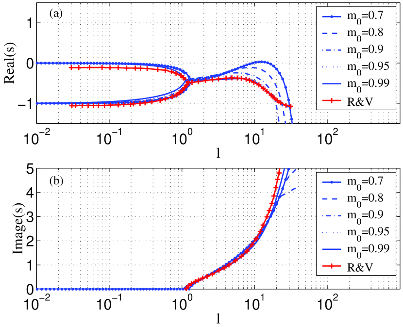
Figure 1.— Perturbation growth rate, s, as function of wave number for various values of $m_{0}$, the fraction of self-similar solution mass contained in the self-similar part of the flow [see eq. (28)], for $\omega=0,\gamma=1.5$. The lines denoted ”R&V” show the results of the analysis of Ryu & Vishniac (1987). The perturbation amplitude evolves as $f\propto t^{{\rm Re}(s)}\exp(i{\rm Im}(s)\ln t)$.

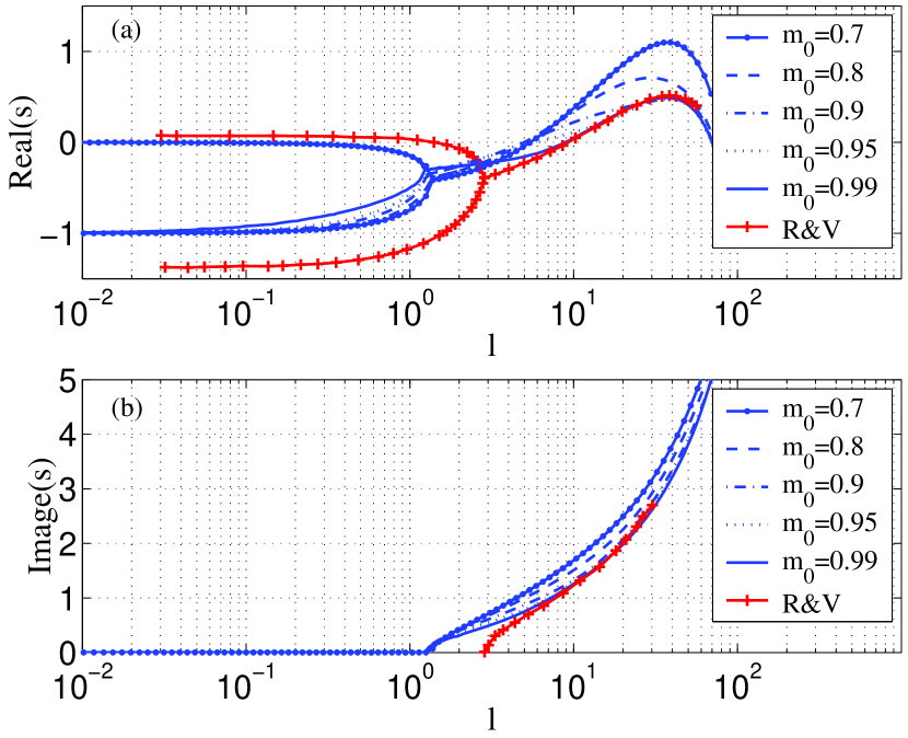
Figure 2.— Perturbation growth rate, s, as function of wave number for various values of $m_{0}$, the fraction of self-similar solution mass contained in the self-similar part of the flow, for $\omega=0,\gamma=1.1$. The lines denoted ”R&V” show the results of the analysis of Ryu & Vishniac (1987). The perturbation amplitude evolves as $f\propto t^{{\rm Re}(s)}\exp(i{\rm Im}(s)\ln t)$.

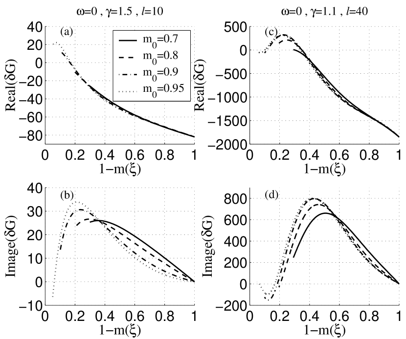
Figure 3.— The real and the imaginary parts of $\delta G$ as function of $1-m(\xi)$, where $m(\xi)$ is the fraction of self-similar solution mass in $[0,\xi]$ [see eq. (28)], for the $\omega=0,\gamma=1.5,l=10$ case ((a)-(b)) and for the $\omega=0,\gamma=1.1,l=40$ case ((c)-(d)). The physical solution oscillates between the real and the imaginary parts.

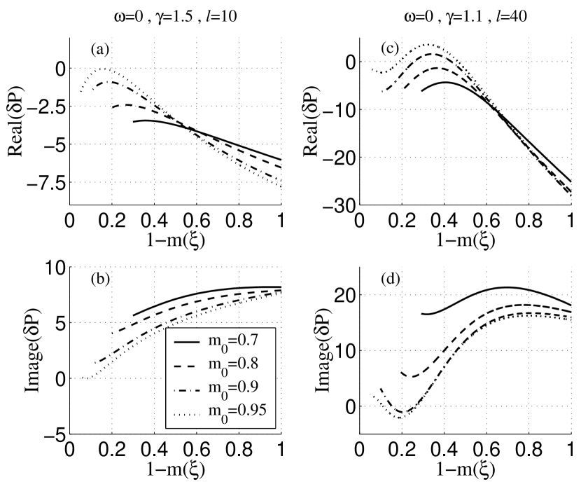
Figure 4.— The real and the imaginary parts of $\delta P$ as function of $1-m(\xi)$, where $m(\xi)$ is the fraction of self-similar solution mass in $[0,\xi]$ [see eq. (28)], for the $\omega=0,\gamma=1.5,l=10$ case ((a)-(b)) and for the $\omega=0,\gamma=1.1,l=40$ case ((c)-(d)). The physical solution oscillates between the real and the imaginary parts.

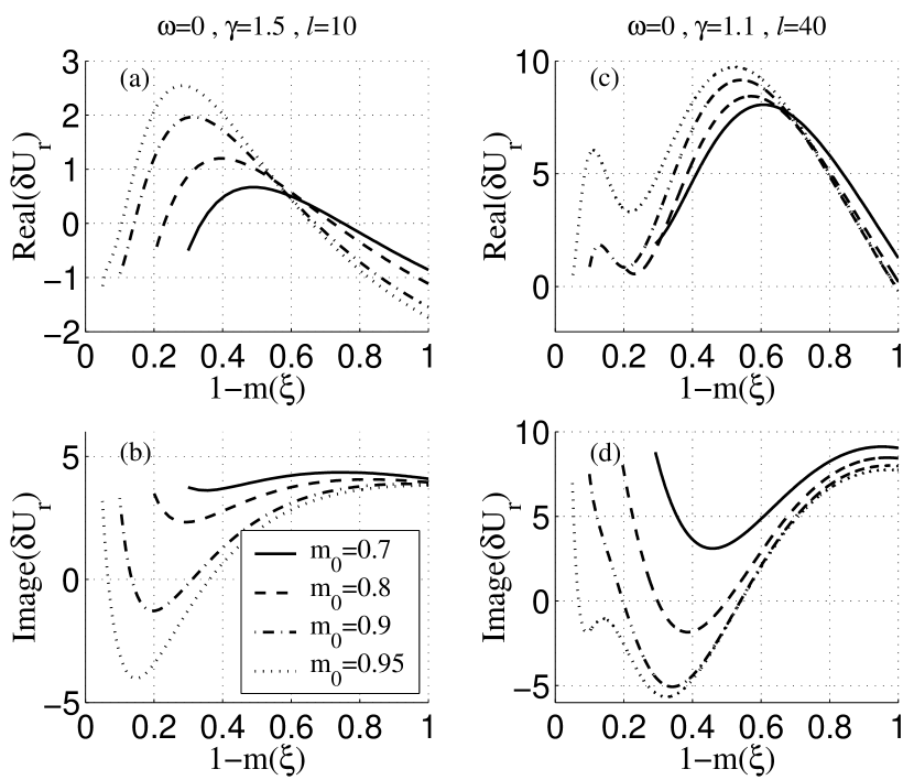
Figure 5.— The real and the imaginary parts of $\delta U_{r}$ as function of $1-m(\xi)$, where $m(\xi)$ is the fraction of self-similar solution mass in $[0,\xi]$ [see eq. (28)], for the $\omega=0,\gamma=1.5,l=10$ case ((a)-(b)) and for the $\omega=0,\gamma=1.1,l=40$ case ((c)-(d)). The physical solution oscillates between the real and the imaginary parts.

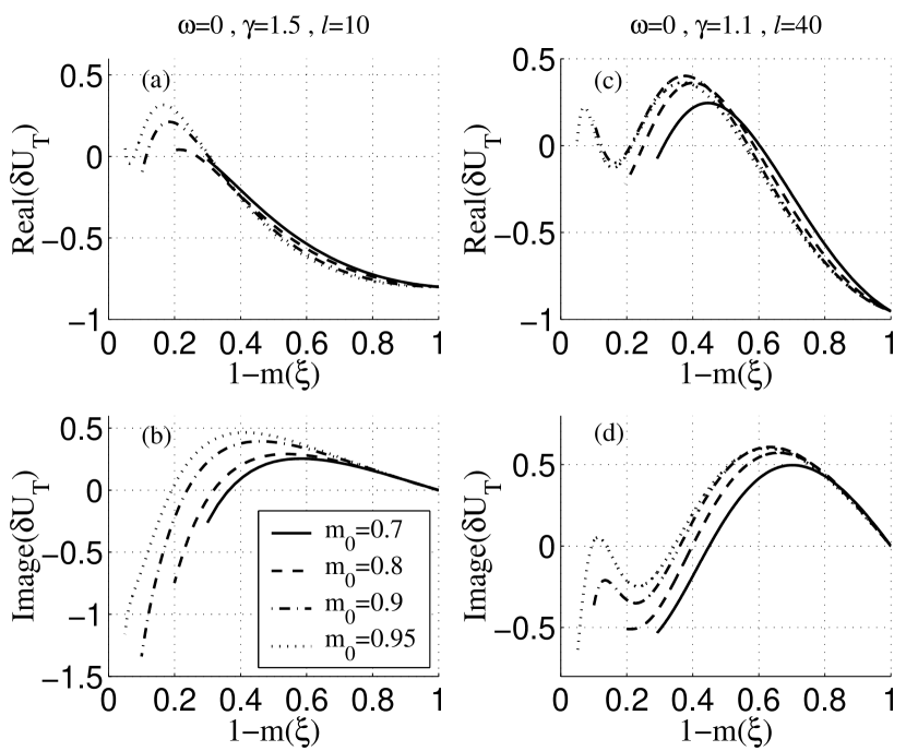
Figure 6.— The real and the imaginary parts of $\delta U_{T}$ as function of $1-m(\xi)$, where $m(\xi)$ is the fraction of self-similar solution mass in $[0,\xi]$ [see eq. (28)], for the $\omega=0,\gamma=1.5,l=10$ case ((a)-(b)) and for the $\omega=0,\gamma=1.1,l=40$ case ((c)-(d)). The physical solution oscillates between the real and the imaginary parts.

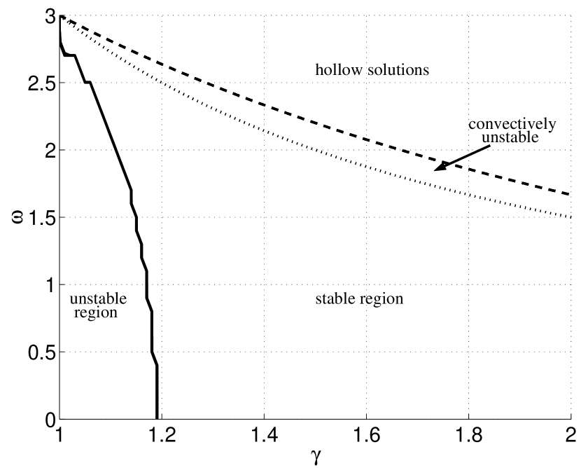
Figure 7.— Stability regions in the $[\omega,\gamma]$ plane: Solid thick line– the asymptotic stability line ($m_{0}\rightarrow 1$); Dotted line– $\omega=3/\gamma$, above which the solutions are convectively unstable. The dashed thick line, $\omega=\omega_{hollow}(\gamma)$ shows the border of the region (top right part of the plane) where the self-similar solutions are hollow, and where our analysis does not apply.

The results for $\omega=0$, i.e. the frequency spectra of the real and imaginary parts of $s$, are shown in figures 1 and 2 for $\gamma=1.5$ and $\gamma=1.1$ respectively. The spatial dependence of the perturbations to the self-similar profiles of flow variables are shown for these cases in figures 3 to 6. The convergence of $s$ to finite values in the limit $m_{0}\rightarrow 1$ justifies the use of the method described in the previous section (see last paragraph of § 3.2). The self-similar, asymptotic solutions are stable for large $\gamma$, and unstable for small $\gamma$. The various stability regions in the $[\omega,\gamma]$ plane are shown in fig. 7. For all values of $\gamma$, the perturbation amplitude shows oscillatory behavior (${\rm Im}(s)\neq 0$) at all but the lowest ($l=1$) wave numbers. These oscillations are dumped (${\rm Re}(s)<0$) in the stable solutions, and amplified (${\rm Re}(s)>0$) over a wide range of wave numbers ($10\lesssim l\lesssim 100$) in the unstable solutions.

The figures demonstrate that a value of $l$, $l=l_{0}$, exists ($l_{0}\cong 2$ for $[\omega=0,\gamma=1.5]$ and $l_{0}\cong 10$ for $[\omega=0,\gamma=1.1]$) such that for $l>l_{0}$ the solutions converge to the Ryu & Vishniac solutions as $m_{0}$ tends to 1. The reason for this convergence is explained in appendix § A. In brief, there is some component of the perturbed solution that diverges at the origin. In this situation, any finite boundary condition forces this component to vanish, thus yielding the correct solution. For $l<l_{0}$, the results of Ryu & Vishniac differ from ours. It is interesting to note here that it was proven by Gurevich & Rumyanstev (1970), using arguments valid for $l\rightarrow 0$ and any $[\omega,\gamma]$, that two stable modes of perturbation exist in this limit, with $s=0$ and $s=-1$ (for details, see appendix § B). Our method of solution reproduces this result, in contrast with the method of Ryu & Vishniac, which does not provide the correct value of $q$ for small wave numbers.

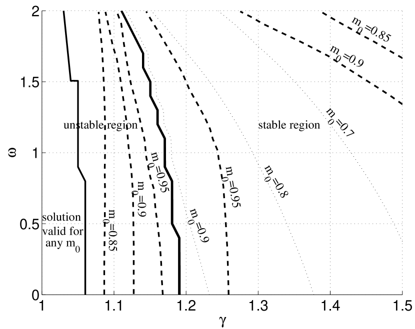
Figure 8.— Regions of validity: The growth rates derived by our analysis are valid for solutions that coincide with the self-similar solution at $\xi_{0}<\xi<1$, provided that the fraction of self-similar solution mass contained in the $[\xi_{0},1]$ region, $m_{0}(\xi_{0})$ [see eq. (28)], is larger than the value indicated by the dashed lines. The thin solid line shows the boundary of the region where the growth rates derived by our analysis are valid for any value of $m_{0}$ [eq. (27) holds for any $m_{0}$]. The thick solid line shows the boundary of the stability region of the asymptotic solutions, $m_{0}\rightarrow 1$, and dotted lines show the marginal stability lines for different $m_{0}$ values, obtained by our analysis. A comparison of these lines with the dashed lines shows that instability at $m_{0}<1$ is obtained in the region of stable asymptotic solutions only for $m_{0}$ values lower than those for which our analysis provides accurate values of the growth rates. This implies that, based on the current analysis, one can not infer the existence of instability for $m_{0}<1$ at regions where the asymptotic, $m_{0}\rightarrow 1$, solutions are stable.

As explained at the end of § 3.2, the value of $s$ obtained for $m_{0}<1$ gives the growth rate for global perturbations to solutions which deviate from the self-similar solution at $\xi<\xi_{0}(m_{0})$, provided the condition given in eq. (27) is satisfied. Figure 8 shows a magnification of figure 7 with contours (dashed lines) indicating values of $m_{0}$ for which equality is obtained between the left hand side and the right hand side of eq. (27), for the wave number $l(\gamma,\omega)$ at which a maximum in $|s|$ is obtained. The growth rates $s$ obtained by our analysis are accurate for $m_{0}$ values larger than those at which equality is obtained. For small $\gamma$ values, e.g. $\gamma<1.06$ for $\omega=0$, our analysis provides accurate $s$ values for arbitrarily small $m_{0}$. Figure 8 demonstrates that, based on the current analysis, one can not infer the existence of instability for $m_{0}<1$ at $[\omega,\gamma]$ regions where the asymptotic, $m_{0}\rightarrow 1$, solutions are stable. However, we find that the flow is in general less stable for smaller $m_{0}$. In the region where the asymptotic solutions, $m_{0}\rightarrow 1$, are stable, we find slower decay rates of the perturbation amplitudes for $m_{0}<1$, compared to the decay rates obtained for the asymptotic solutions. In the region where the asymptotic solutions are unstable, we find growth rates which are larger than those obtained for the unstable asymptotic solutions.

5. Discussion

We have examined the stability of decelerating shocks expanding into ideal gas with density profile decreasing with distance from the origin according to $\rho=Kr^{-\omega}$, for the case where the solutions are not hollow, i.e., $\omega<(7-\gamma)/(\gamma+1)$. We have shown that direct examination of the stability of Sedov-von Neumann-Taylor solutions is not possible due to the divergence of the entropy near the origin (see § 2.2 and § A). Instead, we have analyzed the stability of modified solutions, that coincide with the self-similar solutions at $0<\xi_{0}<\xi=r/R(t)<1$, and deviate from the self-similar solutions at $\xi<\xi_{0}$. We have shown that the global stability of the flow is independent of the details of the solution in the region where it deviates from self-similarity, and obtained the growth rates $s(l,\gamma,\omega)$ [see eq. (18)] of global modes of perturbations by taking the limit $\xi_{0}\rightarrow 0$. Several examples of the dependence of $s(l,\gamma,\omega)$ on $l$ and of the spatial structure of global modes of perturbations are given in figures 1 to 6. The regions of stability in the $[\omega,\gamma]$ plane are outlined in figure 7.

Using our new method of analysis, we have demonstrated that while the growth rates of global modes derived by previous analyses are accurate in the large wave number (small wavelength) limit, they differ significantly from the correct values at low wave numbers (see, e.g. figures 1 and 2). The reasons for the convergence of previous analyses (or any other analysis which require finite inner boundary condition) to the correct values of $s(l,\gamma,\omega)$ at large $l$, and for their failure at small $l$, are explained in appendix A.

The growth rates obtained by our method for finite $\xi_{0}$, $s(l,\gamma,\omega;\xi_{0})$, describe the growth rates of global perturbations for solutions that deviate from the self-similar solutions at $\xi<\xi_{0}$, provided the constraint of Eq. (27) is satisfied. Figure 8 shows the values of $m_{0}(\omega,\gamma)$, the fraction of self-similar solution mass contained in the self-similar part of the flow, $\xi_{0}<\xi<1$ [see eq. (28)], above which this condition is satisfied. For small $\gamma$ values, e.g. $\gamma<1.06$ for $\omega=0$, our analysis provides accurate $s$ values for arbitrarily small $m_{0}$.

Based on the current analysis, one can not infer the existence of instability of the pre-asymptotic flow, i.e. for $m_{0}<1$, at $[\omega,\gamma]$ regions where the asymptotic, $m_{0}\rightarrow 1$, solutions are stable (see figure 8). However, we find that the pre-asymptotic flow is in general less stable than the asymptotic flow. In the stable region of the $[\omega,\gamma]$ plane (figure 8), we find (see figure 1) slower decay rates of the perturbation amplitudes for $m_{0}<1$ ($\xi_{0}>0$), compared to the decay rates obtained for the asymptotic solutions, $m_{0}\rightarrow 1$ ($\xi_{0}\rightarrow 0$). In the unstable region, we find growth rates which are larger than those obtained for the unstable asymptotic solutions (see figure 2). This implies that as the shock wave evolves and approaches self-similarity, the perturbation growth rates are also evolving, and are determined at any given time by the appropriate value of $m_{0}$. For unstable shock waves, the over all growth of perturbations depends on the evolution of $m_{0}$ at early times.

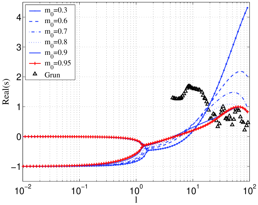
Figure 9.— The real part of the perturbation growth rate, s, as function of wave number for $\omega=0,\gamma=1.06$, compared with the values measured by Grun et al. (1991). The measured values are higher than the growth rates obtained for the asymptotic, $m_{0}\rightarrow 1$, self-similar solutions. However, as explained in the discussion, the flow in the experiment reaches only $m_{0}\lesssim 0.87$.

In the experiment of Grun et al. (1991), the ambient gas adiabatic index was $1.06\pm 0.02$, and the maximum growth rate was $s\cong 1.6$ at $kR\cong 10$ (we will assume $kR\sim l$ though the wave numbers in the experiment were obtained from the projection onto a plane of the edge of an unstable sphere, thus $kR$ is not identical to $l$). The numerical and the experimental results for $\omega=0$ and $\gamma=1.06$ are shown in figure (9) (Note, that our method is valid in this case for any $m_{0}$, see figure 8). The maximal growth rate of perturbations to the asymptotic solution is $s\cong 1$ at $l\cong 60$. The growth rate is larger, however, for $m_{0}\leq 0.7$. We can estimate $m_{0}$ in the experiment from figure 3(a) of Grun et al. (1991). The radius beyond which the shock expands according to the self-similar scaling is $R_{initial}\cong 7mm$, and the perturbations keep growing until $t\cong 200ns$, where the shock radius is $R_{final}\cong 14mm$. Thus, $m_{0}$ is given by $m_{0}(R)=1-(R_{initial}/R)^{3}$, and the maximum value of $m_{0}$ is $m_{0}\approx 0.87$. This implies that the experiment does not measure the asymptotic ($m_{0}\rightarrow 1$) value of $s$, but rather $s(m_{0})$ with $m_{0}<0.87$. This may account for the large growth rates determined by the experiment.

The most unstable modes predicted by our linear analysis are still characterized by larger wave numbers, $l>50$, than obtained by Grun et al. (1991). However, since the growth rates predicted by our analysis for large wave numbers are large, we expect the evolution of perturbations to become non-linear at an early stage. The non-linear interaction at large wave numbers may lead to perturbation amplitudes at smaller wave numbers, $l\sim 10$, which are larger than predicted by linear analysis. Our predictions may be tested in future experiments, by controlling $m_{0}$. For example, lower gas densities or higher ablated material densities will make $m_{0}$ smaller, leading to higher perturbation growth rates.

Finally, we note that for stable asymptotic shocks, e.g. the $[\omega=0,\gamma=5/3]$ case relevant for the ”Sedov-phase” of supernovae shocks, our analysis results do not differ significantly from from those of Ryu & Vishniac. However, since in general we find that the flow is less stable at small $m_{0}$, it is possible that instabilities do arise during the pre-asymptotic stage of shock evolution. This should be checked by numerical simulations.

Appendix A A. The asymptotic behavior for large $m_{0}$ values

As indicated in § 4, our solution for the growth rate $s$ tends to the Ryu & Vishniac solution as $m_{0}$ tends to 1, for sufficiently large $l$, $l>l_{0}$. We explain here the reason for this convergence, and the reason for the deviation of our results from those of Ryu & Vishniac for $l<l_{0}$. Moreover, we will prove that any finite inner boundary condition will yield the correct solution for sufficiently large $l$.

The perturbation eqs. (3.1) can be simplified in the limit $\xi\rightarrow 0$ by using (following Ryu & Vishniac (1987)) the asymptotic behavior, Eq. (2.2), of the self-similar solution in this limit. Assuming that in this limit the perturbations behave as

$$\delta P=\delta P_{0}\xi^{d},\qquad\delta U_{r}=\delta U_{r0}\xi^{d-a},\qquad\delta U_{T}=\delta U_{T0}\xi^{d-a},\qquad\delta G=\delta G_{0}\xi^{d-2},$$ (A1)

a set of four linear equations is obtained for $\delta P_{0},\delta U_{r0},\delta U_{T0}$, and $\delta G_{0}$. In order for a nontrivial solution to exist, the determinant of the coefficient matrix of these equations must vanish,

$$\left|\begin{array}[]{cccc}A_{11}&A_{12}&A_{13}&0\\ A_{21}&A_{22}&0&A_{24}\\ 0&0&A_{33}&A_{34}\\ A_{41}&A_{42}&0&0\end{array}\right|=0,$$ (A6)

where

$$A_{11} = q-\omega+3/\gamma+(d-2)(1/\gamma-1),$$

$$A_{12} = (d+1),$$

$$A_{13} = -l(l+1),$$

$$A_{21} = -aP_{1}/G_{0},$$

$$A_{22} = \delta+q+2/\gamma-1+(1/\gamma-1)(d-a),$$

$$A_{24} = d,$$

$$A_{33} = \delta+q+2/\gamma-1+(1/\gamma-1)(d-a),$$

$$A_{34} = 1,$$

$$A_{41} = -\gamma q+(\gamma-1)(d-a),$$

$$A_{42} = -\gamma(a-2).$$ (A7)

Eq. A6 is therefore a fourth order polynomial equation for $d$. If four different solutions $d$ exist, none of the powers in Eq. A1 is zero, then any solution of the perturbation equations is given, near the origin, by a linear combination of the power-law solutions corresponding to different values of $d$. For $l>l_{0}$, four different solutions to the polynomial eq. for $d$ exist, with only one negative $d-a$ value (the smallest power in Eq. A1). Requiring the pressure to be finite at the origin is equivalent in this case to requiring that the solution be a combination of the 3 approximate solutions corresponding to positive $d-a$ values. This uniquely determines the value of $q$. Thus, the method used by Ryu & Vishniac, seeking solutions that do not diverge near the origin by requiring finite boundary condition, yields the correct value of $q$ for $l>l_{0}$.

In the region $l<l_{0}$, more than one solution with negative $d-a$ exists. In this case, requiring the solution not to diverge at the origin does not yield the correct solution. It is for this reason that the numerical method used by Ryu & Vishniac does not converge to the correct solution of $q$ for $l<l_{0}$. In contrast, our numerical method is free of such difficulties. Note, that in the limit $l\rightarrow 0$, one of the solutions to Eq. A6 is $d=0$, which implies the existence of an additional solution, not of the form given by Eq. A1. This additional solution is given analytically in appendix § B.

Appendix B B. The behavior for small wave numbers

In the self-similar solution, any flow variable $w(r,t)$ (where $w$ may stand, e.g., for $\rho,u,c$) is given in the form $w(r,t)=R^{e_{1}}\dot{R}^{e_{2}}W(\xi)$ where $\xi=r/R$. For the problem under consideration, $R$ is given in the form $R=A(t-t_{0})^{\alpha}$. The parameters $e_{1}$ and $e_{2}$ and the function $W$ depend only on the parameters $\gamma$ and $\omega$ (which determine also the value of $\alpha$). Thus, for given $\gamma,\omega$ the solution depends on only two parameters, $A$ and $t_{0}$.

An approximation to the perturbed solution in the limit of small wave numbers, $l\rightarrow 0$, may be obtained using the following argument (Gurevich & Rumyanstev, 1970). For small wave numbers, large wave lengths, we may assume that the flow along any direction $\theta,\phi$ evolves with time as if it were part of a spherically symmetric solution. This approximation is valid as long as the time scale for the evolution of the perturbation is shorter than the time it takes sound waves to propagate tangentially over a distance $\sim R/l$ over which the deviation from isotropy is appreciable. This approximation gives, of course, the exact solution for $l=0$, and may be expected to provide an approximate description of the behavior at $l\rightarrow 0$. Since the spherically symmetric solution depends on only two parameters, $A$ and $t_{0}$, the perturbed solution is given in this approximation in the form

$$w(r,\theta,\varphi)=R_{p}^{e_{1}}\dot{R}_{p}^{e_{2}}W(r/R_{p}),$$ (B1)

where

$$R_{p}=R(t;A(\theta,\varphi),t_{0}(\theta,\varphi)).$$ (B2)

Here, it is assumed that $A(\theta,\varphi)$ and $t_{0}(\theta,\varphi)$ differ from their values in the spherical solution, $A_{s}$ and $t_{0s}$, only infinitesimally, and that they are slowly varying functions of $(\theta,\varphi)$.

Using spherical harmonics decomposition,

$$A(\theta,\varphi) = A+\delta AY_{lm}(\theta,\varphi),$$

$$t_{0}(\theta,\varphi) = t_{0}+\delta t_{0}Y_{lm}(\theta,\varphi),$$ (B3)

one obtains

$$\delta R(t,\theta,\varphi) = [\frac{\partial R}{\partial A}\delta A+\frac{\partial R}{\partial t_{0}}\delta t_{0}]Y_{lm}(\theta,\varphi),$$

$$\delta w(r,\theta,\varphi) = R^{e_{1}}\dot{R}^{e_{2}}[e_{1}-\xi W^{\prime}+e_{2}\frac{R\delta\dot{R}}{\dot{R}\delta R}]\delta R$$ (B4)

for the deviation from the spherical solution.

From equation (B) it is clear that there are two perturbation modes: one is associated with changes in $t_{0}$, and the other with changes in $A$. Since for $R(t)=A(t-t_{0})^{\alpha}$ we have $\delta R(t)=R({\delta A}/A+{\delta t_{0}}/{(t-t_{0})})$, $s=0$ is obtained for perturbations associated with changes in $A$, and $s=-1$ is obtained for perturbations associated with changes in $t_{0}$.

The radial dependence of the perturbations is given by

$$\delta G(\xi) = [-\omega-\xi G^{\prime}(\xi)/G(\xi)]G(\xi),$$

$$\delta U_{r}(\xi) = [\delta-1-\xi U^{\prime}(\xi)/U(\xi)]U(\xi),$$

$$\delta P(\xi) = [-\omega+2\delta-\xi P^{\prime}(\xi)/P(\xi)]P(\xi)$$ (B5)

for $t_{0}$ associated perturbations, and by

$$\delta G(\xi) = [-\omega-\xi G^{\prime}(\xi)/G(\xi)]G(\xi),$$

$$\delta U_{r}(\xi) = [-\xi U^{\prime}(\xi)/U(\xi)]U(\xi),$$

$$\delta P(\xi) = [2-\omega-\xi P^{\prime}(\xi)/P(\xi)]P(\xi)$$ (B6)

for $A$ associated perturbations.

The tangential velocity perturbation may be obtained by integrating the third equation of (3.1). Since it is proportional to $\mathbf{\nabla_{T}}Y_{lm}(\theta,\varphi)$, the tangential velocity perturbation tends to zero as $l$ tends to zero. It is straight forward to show that for every $\omega$ and $\gamma$ equation (B) is a solution of equations (3.1) with $l=0$ and $s=-1$, and that equation (B) is a solution of equations (3.1) with $l=0$ and $s=0$. This can be most easily inferred from equation (6), equation (8), and energy conversation,

$$C^{2}=\frac{\gamma(\gamma-1)}{2}\frac{U^{2}(1-U)}{\gamma U-1}.$$ (B7)

References

- Chevalier (1990) Chevalier, R. A. 1976, ApJ, 359, 463
- Cox (1980) Cox, J. P. 1980, Theory of Stellar Pulsation (Princeton: Princeton Univ. Press)
- Erpenbeck (1962) Erpenbeck, J. J. 1962, Phys. Fluids, 5, 1181
- Hansen et al. (2002) Hansen, J. F. et al. 2002, 2002APS..DDPPGP1060H
- Goodman (1990) Goodman, J. 1990, ApJ, 358, 214
- Grun et al. (1991) Grun, J. et al. 1999, Phys. Rev. Lett., 66, 2738
- Gurevich & Rumyanstev (1970) Gurevich, L. E., & Rumyanstev, A. A. 1970, Soviet Physics-Astronomy, 13, 908
- Laming & Grun (2002) Laming, j. M., & Grun, J. 2002, Phys. Rev. Lett., 89, 125002
- Laming & Grun (2003) Laming, j. M., & Grun, J. 2003, Phys. Plasmas, 10, 1614
- Landau & Lifshitz (1987) Landau, L. D., & Lifshitz, E. M. 1987, Fluid Mechanics (Oxdord:Pergamon Press)
- Mac Low & Norman (1993) Mac Low, M. M., & Norman, L. N. 1993, ApJ, 407, 207
- Meyer-ter-Vehn (1982) Meyer-ter-Vehn, J., & Schalk, C. 1982, Z. Naturforsch, 37a, 955
- Ostriker & McKee (1988) Ostriker, J. P. & Mckee, C. F. 1988, Rev. Mod. Phys. 60, 1
- Ryu & Vishniac (1987) Ryu, D., & Vishniac, E. T. 1987, ApJ, 313, 820
- Ryu & Vishniac (1991) Ryu, D., & Vishniac, E. T. 1991, ApJ, 368, 411
- Sari, Waxman & Shvarts (2000) Sari, R., & Waxman, E., & Shvarts, D. 2000, ApJS, 127, 475
- Sedov (1946) Sedv, L. I. 1946, Prikl. Mat. i Mekh., 10, 241
- Taylor (1950) Taylor, G. I. 1950, Proc. R. Soc. London A, 201, 159
- Von Neumann (1947) Von Neumann, J. 1947, Los Alamos Sci. Lab. Tech. Se., 7
- Waxman & Shvarts (1993) Waxman, E., & Shvarts, D. 1993, Physics of Fluids A, 5, 1035
- Zèldovich & Raizer (1968) Zèldovich, Ya. B., & Raizer, Yu. P. 1968, Physics of Shock Waves and High-Temperature Hydrodynamic Phenomena (New York:Academic)