Rotochemical Heating in Millisecond Pulsars.
Formalism and Non-superfluid case.

Abstract

Rotochemical heating originates in a departure from beta equilibrium due to spin-down compression in a rotating neutron star. The main consequence is that the star eventually arrives at a quasi-equilibrium state, in which the thermal photon luminosity depends only on the current value of the spin-down power, which is directly measurable. Only in millisecond pulsars the spin-down power remains high long enough for this state to be reached with a substantial luminosity. We report an extensive study of the effect of this heating mechanism on the thermal evolution of millisecond pulsars, developing a general formalism in the slow-rotation approximation of general relativity that takes the spatial structure of the star fully into account, and using a sample of realistic equations of state to solve the non-superfluid case numerically. We show that nearly all observed millisecond pulsars are very likely to be in the quasi-equilibrium state. Our predicted quasi-equilibrium temperatures for PSR J0437-4715 are only 20% lower than inferred from observations. Accounting for superfluidity should increase the predicted value.

1 INTRODUCTION

Neutron star cooling is an important tool for the study of dense matter. By comparing cooling models with observations of thermal emission from these objects, we can gain insight into the equation of state (EOS) of dense matter, the signatures of exotic particles, superfluid energy gaps, and magnetic field properties [for a recent review, see Yakovlev & Pethick (2004)]. A neutron star loses the thermal energy with which it was born initially through neutrino emission, and later through photon emission, the change between these two stages occurring about $10^{5}$ yr after birth.

Several heating mechanisms may become important during late stages of the evolution of a neutron star, most of them related to the delayed adjustment to the progressively changing equilibrium state as the rotation slows down. These include the dissipation of rotational energy due to interactions between superfluid and normal components of the star (Shibazaki & Lamb, 1989) and release of strain energy stored by the solid crust due to spin-down deformation (Cheng et al., 1992).

Another of these mechanisms is rotochemical heating (Reisenegger, 1995), which has its origin in deviations from beta equilibrium due to spin-down compression. As a neutron star spins down, the centrifugal force acting on each fluid element diminishes, changing the local value of the pressure. Since the composition of neutron star matter in beta equilibrium is a one-parameter function, this compression results in a displacement of the equilibrium concentration of each particle species. Reactions which change the chemical composition are in charge of driving the system to the new equilibrium configuration. But if the rate at which reactions do this task is slower than the change of the equilibrium concentrations due to spin-down compression, the system is permanently out of chemical equilibrium. This implies an excess of energy, which is dissipated by enhanced neutrino emission and heat generation.

After its introduction, this heating mechanism was studied by several authors: Cheng & Dai (1996) applied it to quark stars, Reisenegger (1997) made an order-of-magnitude estimate of the effects of superfluidity, and Iida & Sato (1997) studied the heating due to compositional transitions in the crust due to spin-down compression. All studies agree that rotochemical heating is particularly important for old neutron stars with fast rotation and low magnetic fields, features that are characteristic of millisecond pulsars (MSPs).

The most striking prediction associated with rotochemical heating is that, if the spin-down timescale is substantially longer than any other timescale involved (with the likely exception of magnetic field decay), the star arrives at a quasi-equilibrium state, in which the temperature depends only on the current, slowly changing value of $\Omega\dot{\Omega}$ (the product of the angular velocity and its time derivative), proportional to the spin-down power, and not on the star’s previous history (Reisenegger, 1995). This provides a simple way to constrain the physics involved in theoretical models, once the spin parameters and observed surface temperature of a MSP are known.

Although the qualitative behavior of the thermal evolution of neutron stars with rotochemical heating is known, all previous studies made only order-of-magnitude estimates, ignoring the spatial structure of the star and thus not offering reliable predictions to be compared with observations. Also unknown is the dependence of the thermal evolution on EOS and stellar mass.

In this work, we calculate the thermal evolution of MSPs with rotochemical heating, taking the structure of the star fully into account in the frame of general relativity, and using realistic EOSs of dense matter. In order to do so, we develop a general formalism to treat the evolution of the temperature and departures of chemical equilibrium. As a first approach, we have chosen the simplest possible core composition, namely neutrons, protons, electrons, and muons ($npe\mu$ matter), to see if we can explain observations with it, before invoking exotic particles. The main difficulty of treating the spatial structure of the star is the lack of an expression for the spin-down compression in the frame of general relativity. We develop such an expression with the aid of the slow-rotation approximation of Hartle (1967). The astrophysical situation to be modelled is the stage after the accretion-driven spin-up of the pulsar has finished.

Although it is generally believed that crusts and cores of neutron stars have superfluid components (e.g., Yakovlev & Pethick 2004), in this work we ignore superfluidity. Our plan is to make an extensive study of rotochemical heating in non-superfluid stars and compare results with observations, in order to assess whether invoking superfluidity (whose parameters are currently very uncertain) is necessary to explain observations.

The structure of this paper is the following: In §2, we develop our general formalism, as well as the expression for the spin-down compression rate. In §3, we detail the input necessary for numerical calculations (EOS, reactions, heat capacities, etc.). In §4, we describe our results, comparing our predictions with the recent detection of likely thermal ultraviolet emission from the nearest MSP, PSR J0437-4715 (Kargaltsev, Pavlov, & Romani, 2004), and the lack of optical emission from the even closer “classical” pulsar PSR J0108-1413 (Mignani, Manchester, & Pavlov, 2003). We also list some other MSPs for which the rotochemical heating luminosity might become detectable. A short summary of our main conclusions is given in §5.

2 THEORETICAL FRAMEWORK

2.1 Basic Equations

It is conventional in neutron star cooling calculations to divide the star into two regions: a nearly isothermal interior, which ranges from the center out to density $\rho_{b}\sim 10^{10}$ g cm^-3, and a thin envelope, which ranges from $\rho_{b}$ to the surface and where a strong temperature gradient exists (Gudmundsson, Pethick, & Epstein, 1983). Since we are modelling the thermal evolution of a MSP long after accretion has stopped, it is safe to assume that thermal relaxation from an initial non-uniform internal temperature profile has already occurred, so that the redshifted internal temperature,

$$T_{\infty}=T(r)e^{\Phi(r)},$$ (1)

is uniform (see, e.g., Glendenning 1997). Here, $g_{tt}=-e^{2\Phi}$ is the time component of the metric of a non-rotating reference star, of which $r$ is the radial spherical coordinate. Although spherical symmetry is broken for a rotating star, we describe the latter as a perturbation to the corresponding non-rotating star (with the same total baryon number). We establish a Lagrangian correspondence between the surfaces of constant $r$ in the non-rotating star with the constant-pressure surfaces of its rotating counterpart, on which all local thermodynamic quantities will be shown to be constant (see § 2.2). The evolution of the internal temperature is given by the thermal balance equation (Thorne, 1977), which for an isothermal interior is given by

$$\dot{T}_{\infty}=\frac{1}{C}\left[L^{\infty}_{H}-L^{\infty}_{\nu}-L^{\infty}_{\gamma}\right],$$ (2)

where $C$ is the total heat capacity of the star, $L^{\infty}_{H}$ is the total power released by heating mechanisms, $L^{\infty}_{\nu}$ is the total neutrino luminosity, and $L^{\infty}_{\gamma}$ is the photon luminosity. These quantities are calculated as

$$C = \sum_{i}\int dVc_{V,i},$$ (3)

$$L_{H}^{\infty} = \int dVQ_{H}e^{2\Phi},$$ (4)

$$L_{\nu}^{\infty} = \int dVQ_{\nu}e^{2\Phi},\textrm{ and}$$ (5)

$$L_{\gamma}^{\infty} = 4\pi\sigma R^{2}T_{s}^{4}e^{2\Phi_{s}}=4\pi\sigma R_{\infty}^{2}(T_{s}^{\infty})^{4},$$ (6)

respectively, where $dV=4\pi r^{2}\sqrt{g_{rr}}dr$ is the proper volume element, $c_{V,i}$ is the specific heat (heat capacity per unit volume) of each particle species, $Q_{\nu}$ is the total neutrino emissivity contributed by reactions, $Q_{H}$ is the total heating rate per unit volume, $\sigma$ is the Stefan-Boltzmann constant, $R$ is the stellar coordinate radius, $\Phi_{s}=\Phi(R)$, $R_{\infty}=Re^{-\Phi_{s}}$ is the effective radius as measured from infinity, and $T_{s}^{\infty}$ the redshifted effective temperature. The surface temperature $T_{s}$ is obtained from the internal temperature by assuming an envelope model (Gudmundsson et al., 1983; Potekhin et al., 1997).

Since the neutrino emissivity and heating rate are modified when the neutron star is out of chemical equilibrium (Haensel, 1992; Reisenegger, 1995), the evolution of the temperature depends on how strongly it departs from the beta equilibrium state. For $npe\mu$ matter, this departure can be quantified by the chemical imbalances (Haensel, 1992):

$$\eta_{npe} = \delta\mu_{n}-\delta\mu_{p}-\delta\mu_{e},$$ (7)

$$\eta_{np\mu} = \delta\mu_{n}-\delta\mu_{p}-\delta\mu_{\mu},$$ (8)

where $\delta\mu_{i}=\mu_{i}-\mu_{i}^{eq}$ is the deviation from the equilibrium chemical potential of species $i$, at a given pressure. Since diffusion timescales are short compared with the evolutionary timescales to be considered (Reisenegger, 1997), we assume uniform redshifted chemical potential deviations throughout the core:

$$\delta\mu_{i}^{\infty}\equiv\delta\mu_{i}(r)e^{\Phi(r)}.$$ (9)

To obtain the time evolution of the chemical imbalances, we start by writing down the chemical potential of each particle species as a function of the number density of all particles: $\mu_{i}=\mu_{i}(\left\{n_{j}\right\})$. We assume small departures from chemical equilibrium, which can be expressed by requiring that $|\delta\mu_{i}|\ll\mu_{i}^{eq}$. In this approximation, the departures from the equilibrium particle number densities $\delta n_{i}=n_{i}-n_{i}^{eq}$ are related to the $\delta\mu_{i}$ by

$$\delta n_{i}=\sum_{j}\frac{\partial n_{i}}{\partial\mu_{j}}\delta\mu_{j},$$ (10)

where the partial derivatives are evaluated at the beta equilibrium state. To eliminate the effect of particle diffusion between different regions of the star, we integrate equation (10) over regions where free particles exist. After integration, we obtain the deviation from the equilibrium number of particles $\delta N_{i}$ as a function of the redshifted chemical potential lags:

$$\delta N_{i}=\sum_{j}B_{ij}\delta\mu_{j}^{\infty},$$ (11)

with

$$B_{ij}=\int_{core}dV\frac{\partial n_{i}}{\partial\mu_{j}}e^{-\Phi},$$ (12)

where we have used equation (9). Since the $B_{ij}$ do not depend on time, we invert and take the time derivative of equation (11), obtaining the evolution of the $\delta\mu^{\infty}_{i}$:

$$\delta\dot{\mu}_{i}^{\infty}=\sum_{j}\left(B^{-1}\right)_{ij}\delta\dot{N}_{j}.$$ (13)

The rate of change of $\delta N_{i}$ is given by

$$\delta\dot{N}_{i}=\dot{N}_{i}-\dot{N}_{i}^{eq},$$ (14)

where

$$\dot{N}_{i}=\int_{core}dVe^{\Phi}\sum_{\alpha}\Delta\Gamma^{i}_{\alpha}$$ (15)

is the change in the total number of particles of species $i$ due to reactions (Thorne, 1977). Here, $\Delta\Gamma^{i}_{\alpha}$ is the net creation rate of particles of species $i$ per unit volume due to reaction $\alpha$. It can be checked that the $\dot{N_{i}}$ satisfy baryon number and charge conservation. The quantity $\dot{N}_{i}^{eq}$ is the change in the equilibrium value of the total number of particles of species $i$, which depends on the spin-down compression rate. We defer its calculation to the next subsection. The evolution of the redshifted chemical imbalances $\eta^{\infty}=\eta(r)e^{\Phi}$ follows from equations (7), (8), and (9):

$$\dot{\eta}^{\infty}_{npe}=\delta\dot{\mu}^{\infty}_{n}-\delta\dot{\mu}^{\infty}_{p}-\delta\dot{\mu}^{\infty}_{e}$$ (16)

$$\dot{\eta}^{\infty}_{np\mu}=\delta\dot{\mu}^{\infty}_{n}-\delta\dot{\mu}^{\infty}_{p}-\delta\dot{\mu}^{\infty}_{\mu}$$ (17)

Equations (2), (16), and (17) give a complete description of the thermal evolution of a neutron star with rotochemical heating and $npe\mu$ composition, given an expression for $\dot{N}_{i}^{eq}$.

2.2 Lagrangian Spin-down Compression Rate

For slow enough rotation frequencies, the deviation of the star from the non-rotating configuration can be treated as a small perturbation, which we describe in terms of a Lagrangian formalism. Using the fact that the total baryon number $A$ of a star is conserved, we can describe its interior in terms of surfaces of constant pressure $P$ enclosing a fixed number of baryons $N$ (e.g., the surface $P=0$ encloses $A$ baryons inside it). As the stellar rotation rate changes, these surfaces will readjust their shapes, with a corresponding change in $P$, but keeping $N$ constant. Since there is a one-to-one relation between the enclosed number of baryons $N$ and the radial coordinate of the non-rotating configuration $r$ (for fixed $A$), we use them interchangeably to identify a given surface, relating them by $dN=4\pi r^{2}\sqrt{g_{rr}}ndr$.

The underlying assumption is that, on a surface of constant pressure, the other thermodynamical quantities are also constant. This is straightforward for neutron-star matter in beta equilibrium (described by a barotropic equation of state), but not so obvious for departures from this state (which are not necessarily barotropic, as the pressure-density relation will also depend on the local particle abundances). We show in Appendix A that, in a uniformly rotating, perfect-fluid star in hydrostatic equilibrium, surfaces of constant pressure coincide with those of constant energy density and gravitational redshift, regardless of whether the equation of state is barotropic. This, together with diffusive equilibrium (uniform redshifted chemical potentials everywhere in the stellar interior), ensures that the chemical composition on each surface is also constant.

To quantify the spin-down compression rate and thus $\dot{N}^{eq}_{i}$, we need an expression for the change in pressure with rotation frequency on each surface enclosing a constant $N$, keeping $A$ constant. Hartle (1967) developed a perturbative approach in the frame of general relativity, relating quantities on rotating and non-rotating stars with the same central energy density $\rho_{c}$ (but, therefore, different $A$), by expanding the metric of an axially symmetric non-rotating star in even powers of the angular velocity $\Omega$. This perturbative approach is valid for stars rotating at frequencies much smaller than the Kepler frequency $\Omega_{K}$, at which mass shedding from the equator occurs. For realistic equations of state, this limiting frequency can be well approximated by means of empirical formulae (Lasota, Haensel, & Abramowicz, 1996). The corresponding Kepler periods, $P_{K}$, are lower than the shortest MSP periods measured to date [see, e.g., The ATNF Pulsar Catalogue (Hobbs et al., 2004)]. Our task is to express our spin-down compression rate at constant $A$ in terms of Hartle’s results, which assume constant $\rho_{c}$.

If the baryon number enclosed by a surface of constant pressure $P$ in a rotating star is $N=N(A,P,\Omega^{2})$, some partial-derivative manipulation yields

$$\left(\frac{\partial P}{\partial\Omega^{2}}\right)_{N,A} = -\frac{(\partial N/\partial\Omega^{2})_{P,A}}{(\partial N/\partial P)_{\Omega^{2},A}}$$ (18)

$$= -\frac{1}{\left({\partial N}/{\partial P}\right)_{\Omega^{2},A}}\left\{\left(\frac{\partial N}{\partial\Omega^{2}}\right)_{P,\rho_{c}}-\left(\frac{\partial N}{\partial\rho_{c}}\right)_{P,\Omega^{2}}\frac{\left({\partial A}/{\partial\Omega^{2}}\right)_{\rho_{c}}}{\left({\partial A}/{\partial\rho_{c}}\right)_{\Omega^{2}}}\right\},$$

where the subscripts denote quantities which are kept constant in carrying out the differentiation. We note that $(\partial A/\partial\Omega^{2})_{\rho_{c}}$ and $(\partial A/\partial\rho_{c})_{\Omega^{2}}$ are just $(\partial N/\partial\Omega^{2})_{P,\rho_{c}}$ and $(\partial N/\partial\rho_{c})_{P,\Omega^{2}}$, respectively, evaluated at the surface of the star ($P=0$). Also, since we are perturbing around the non-rotating configuration, we can evaluate all the derivatives at $\Omega=0$.

Hartle (1967) found that the lowest-order change in a given stellar property with rotation is linear in the squared angular frequency $\Omega^{2}$, for a star with fixed central density. We can thus write

$$\left(\frac{\partial N}{\partial\Omega^{2}}\right)_{P,\rho_{c}}=\frac{N(\rho_{c},P,\Omega^{2})-N(\rho_{c},P,0)}{\Omega^{2}},$$ (19)

and consider it independent of $\Omega^{2}$. To find the number of baryons enclosed by a surface of constant pressure, we recall the baryon number conservation law (Misner & Sharp, 1964), and write

$$N=\int_{V}(-g)^{1/2}u^{t}nd^{3}x,$$ (20)

where $g$ is the determinant of the metric, $u^{t}$ is the time component of the fluid’s four-velocity, $n$ is the rest frame baryon number density, and $V$ is the spatial volume enclosed by the constant pressure surface (throughout this section, we use $G=c=1$). For the non-rotating case, we have

$$N(\rho_{c},P,0)=\int_{0}^{r(\rho_{c},P)}4\pi y^{2}e^{\Lambda(\rho_{c},y)}n(\rho_{c},y)dy,$$ (21)

where $g_{rr}=e^{2\Lambda}=(1-2M/r)^{-1}$ is the radial component of the non-rotating metric. For the rotating case, one has to express the perturbed metric of Hartle (1967) in the non-rotating coordinate system. Keeping terms to order $\Omega^{2}$, we get

$$\left(-g\right)^{-1/2} = e^{\Phi+\Lambda}r^{2}\sin{\theta}\left[1+\frac{m}{r-2M}+h+\xi\frac{d}{dr}\left(\Phi+\Lambda\right)+\frac{2\xi}{r}+2k+\frac{\partial\xi}{\partial r}\right]$$ (22)

$$u^{t} = e^{-\Phi}\left[1-\xi\frac{d\Phi}{dr}-h+\frac{1}{2}r^{2}\sin^{2}{\theta}{\bar{\omega}}^{2}e^{-2\Phi}\right],$$ (23)

where $m$, $h$, and $k$ are metric-perturbing functions which are proportional to $\Omega^{2}$ and can be separated into spherical and quadrupolar parts, $\bar{\omega}$ is the difference between the star’s rotation frequency and the frame-dragging frequency, and $\xi$ is a Lagrangian displacement that relates surfaces of constant $\rho$ in rotating and non-rotating stars of the same $\rho_{c}$ (Hartle, 1967). The spherical polar angle is $\theta$, and the mass enclosed inside the radius $r$ is $M$. Replacing equations (22) and (23) in (20), keeping terms to order $\Omega^{2}$, taking the angular integral, and integrating by parts in $r$, we get

$$N(\rho_{c},P,\Omega^{2}) = \int_{0}^{r(\rho_{c},P)}4\pi y^{2}e^{\Lambda(\rho_{c},y)}n(\rho_{c},y)\left[1+\frac{m_{0}}{y-2M}+\frac{1}{3}y^{2}\bar{\omega}^{2}e^{-2\Phi}\right.$$ (24)

$$\left.-\frac{\xi_{0}(\rho_{c},y)}{n(\rho_{c},y)}\left(\frac{\partial n}{\partial y}\right)_{\rho_{c}}\right]dy+4\pi r^{2}e^{\Lambda(\rho_{c},r)}\xi_{0}(\rho_{c},r)n(\rho_{c},r).$$

The functions $\bar{\omega}$, $m_{0}$, $\xi_{0}$ are obtained by solving first and second-order differential equations in the coordinate $r$, as explained in Hartle (1967), and which need a value for the rotation rate of the star $\Omega$ and a non-rotating relativistic stellar structure as input. The zero subscript on functions indicates their spherical part (the quadrupolar part vanishes when performing the angular integral, and the function $k$ has no spherical part).

The remaining derivatives in equation (18) can be obtained from the non-rotating configuration. We first have

$$\left(\frac{\partial N}{\partial P}\right)_{\Omega^{2},A}=\frac{4\pi r^{2}e^{\Lambda}n}{dP/dr},$$ (25)

where $dP/dr$ can be calculated analytically from the relativistic stellar structure equations (Oppenheimer & Volkoff, 1939). The other derivative has to be obtained by differentiating equation (21):

$$\left(\frac{\partial N}{\partial\rho_{c}}\right)_{P,\Omega^{2}} = 4\pi r^{2}e^{\Lambda(\rho_{c},r)}n(\rho_{c},r)\left(\frac{\partial r}{\partial\rho_{c}}\right)_{P}$$ (26)

$$+\int_{0}^{r}4\pi y^{2}\left[e^{\Lambda(\rho_{c},y)}\left(\frac{\partial n}{\partial\rho_{c}}\right)_{y}+\frac{n(\rho_{c},y)e^{3\Lambda(\rho_{c},y)}}{y}\left(\frac{\partial M}{\partial\rho_{c}}\right)_{y}\right]dy.$$

For numerical calculations, it is convenient to write the derivative in the first term of the right-hand side as

$$\left(\frac{\partial r}{\partial\rho_{c}}\right)_{P}=-\frac{(\partial P/\partial\rho_{c})_{r}}{(\partial P/\partial r)_{\rho_{c}}},$$ (27)

in order to calculate the three derivatives with constant $r$ in the same way.

The resulting spin-down compression rate, equation (18), is plotted in Figure 1, normalized by pressure and Kepler frequency. The left panel displays results obtained for different EOSs, with fixed central pressure, while the right panel shows results for different stellar models and fixed EOS. As expected, the expression is negative, since spin-down compression means increase in $P$ with decrease of $\Omega^{2}$. Compression is strongest at the center of the star. It can be shown that the central value is given by

$$\left(\frac{\partial P}{\partial\Omega^{2}}\right)_{N,A}\mathop{\longrightarrow}\limits_{r\to 0}-\frac{P_{c}\gamma_{c}(\rho_{c}+P_{c})}{\rho_{c}n_{c}}\frac{(\partial A/\partial\Omega^{2})_{\rho_{c}}}{(\partial A/\partial\rho_{c})_{\Omega^{2}}},$$ (28)

where $\gamma=d\log{P}/d\log{\rho}$ is the adiabatic index, and the subscripts $c$ mean central values. Since $(\partial A/\partial\rho_{c})_{\Omega^{2}}=0$ for the maximum mass non-rotating configuration, the divergence of the result for $M\to M_{max}$, as shown in the right panel of Figure 1, is easy to understand. The graphs confirm the order-of-magnitude expression

$$\left(\frac{\partial P}{\partial\Omega^{2}}\right)_{N,A}\sim-\frac{P}{\Omega_{K}^{2}}$$ (29)

which implies that the perturbation is small as long as $\Omega\ll\Omega_{K}$.

With our expression for the spin-down compression rate at hand, we can write the change in the equilibrium number of particles of species $i$ with time as

$$\dot{N}_{i}^{eq}=2\Omega\dot{\Omega}\int_{core}dN\frac{dY^{eq}_{i}}{dP}\left(\frac{\partial P}{\partial\Omega^{2}}\right)_{N,A}\equiv 2\Omega\dot{\Omega}I_{\Omega,i},$$ (30)

where the derivative $dY^{eq}_{i}/dP$ is calculated in beta equilibrium. It is straightforward to check that the $\dot{N}_{i}^{eq}$ satisfy baryon number and charge conservation.

2.3 Effect of a Phase Transition

The variables $N$ and $P$ are clearly continuous functions of $r$ in the non-rotating star, regardless of the presence of a phase transition. In Appendix B, we show explicitly that the same is true for $(\partial P/\partial\Omega^{2})_{N,A}$. On the other hand, the equilibrium particle concentrations may have a discontinuous jump $\Delta Y^{eq}_{i}$ at the transition, which would contribute a Dirac delta function to $dY_{i}^{eq}/dP$. Therefore, there would be a finite contribution to $\dot{N}_{i}^{eq}$ from the transition,

$$\dot{N}_{i}^{eq}|_{trans}=2\Omega\dot{\Omega}\Delta Y^{eq}_{i}\left[\frac{dN}{dP}\left(\frac{\partial P}{\partial\Omega^{2}}\right)_{N,A}\right]_{trans}.$$ (31)

To order of magnitude, the fractional contribution of a phase transition to the total value of $\dot{N}_{i}^{eq}$ (and to the total heating of the star, if the reactions are of the same kind everywhere) is the ratio of the jump $\Delta Y^{eq}_{i}$ to the total variation in $Y^{eq}_{i}$ across the stellar core. In the present work, as described in the following sections, phase transitions are not important, as the only transition in one of our EOSs is fairly weak. In other cases, such as a star with a core of deconfined quarks of fairly uniform relative abundances, the phase transition may dominate the heating.

In order to maintain diffusive equilibrium, a finite number of particles per unit time, $\dot{N}_{i}^{eq}|_{trans}$, must be brought to (or, if negative, away from) the phase transition much faster than the latter progresses due to the spin-down of the star. Therefore, a phase transition is the place where our assumption of diffusive equilibrium is most strongly put into question. However, in the case of interest to us, the low temperatures (implying long mean-free paths and therefore fast diffusion) and the extremely slow evolution should still validate this approximation.

Glendenning (1992) has shown that, due to the presence of two separate conserved charges (baryon number and electric charge), phase transitions in neutron stars may not occur as a single discontinuity, but instead through a mixed phase, in which both phases coexist over a finite range in pressure (or stellar radius). In this case, any discontinuities would be considerably weakened, if not fully eliminated, and we do not expect any special effects (such as discussed above) associated with the phase transitions.

3 INPUT FOR THE NON-SUPERFLUID CASE

To implement the formalism of §2 numerically for the non-superfluid case, we need as input an EOS, neutrino emissivities, a specific heat, and an envelope model. We then have to calculate the stellar structure and the corresponding integrals over the star.

3.1 Equations of State

Since our formalism requires a detailed knowledge of the structure of the star, we need an EOS to determine the spatial dependence of the thermodynamical quantities by solving the relativistic stellar structure equations (Oppenheimer & Volkoff, 1939). In addition to the usual variables given in most published EOSs (pressure, energy density, chemical composition, and adiabatic index, all evaluated in chemical equilibrium), we need to know the partial derivatives of equation (10) (which are easy to compute if we know the energy density or energy per baryon of interacting particles as a function of baryon number density and proton fraction) and the baryon effective masses for computing reaction rates and heat capacities. We also want to cover a broad range of EOSs, in order to assess the dependence of the quasi-equilibrium temperature on their properties. Given our requirements, we have used three sets of EOSs:

1. the two most realistic EOSs from Akmal, Pandharipande, & Ravenhall (1998) (APR) for the core, supplemented with that of Pethick, Ravenhall & Lorentz (1995) and Haensel & Pichon (1994), for the inner and outer crust, respectively;

2. five representative EOSs from Prakash, Ainsworth & Lattimer (1988) (BPAL) for the core, with the same EOSs for the inner and outer crust as for the previous set; and

3. a non-interacting Fermi gas (see, e.g., Shapiro & Teukolsky 1983) for the whole star.

In Table 1 we list, for each EOS, the mass $M$, central energy density $\rho_{c}$, coordinate radius $R$, and effective radius as seen from infinity $R_{\infty}$ of the maximum-mass non-rotating configuration.

Since in the APR set the thermodynamical quantities are obtained from an analytical fit to tabulated many-body calculations (Akmal et al., 1998), care has to be taken when interpreting results obtained for densities higher than the highest tabulated value, since extrapolation can lead to significant errors. This is the reason why we do not list the maximum-mass configuration for the A18 + $\delta\upsilon$ EOS. Another feature of this set is that the A18 + $\delta\upsilon$ + UIX* EOS becomes non-causal at densities greater than $2\times 10^{15}\rm{g\,cm}^{-3}$, which is the central density of a star of $2.14M_{\sun}$, slightly below the maximum mass formally allowed for this EOS, $M_{max}=2.19M_{\sun}$. However, this EOS is considered to be the state of the art among those derived from non-relativistic potentials, since it incorporates three-nucleon interactions and relativistic boost corrections (Akmal et al., 1998). For this reason, we will in what follows take it as our reference EOS.

The EOSs of the BPAL set are labelled according to Prakash et al. (1997), who characterize them by the different magnitude of their nuclear incompressibility and density dependence of their symmetry energy. The values for the Fermi gas EOS listed in Table 1 correspond to a central density slightly below the appearance of $\Sigma^{-}$ hyperons.

The A18 + $\delta\upsilon$ + UIX* EOS has an additional feature: a phase transition associated with the appearance of a neutral pion condensate at a density $\sim 4\times 10^{14}$ g cm^-3. In order to connect the normal phase with the pion-condensed one, we assumed a Maxwell transition, which implies a discontinuity in all thermodynamical quantities but the temperature, pressure and neutron chemical potential, resulting in an energy-density jump of 6.6%. Akmal et al. (1998) also considered the possibility of a mixed-phase transition (e.g., Glendenning 1992), concluding that (for a standard, $1.4M_{\sun}$ neutron star) the shell containing the mixed phase is only $\sim 40$ m thick. They also estimated the Debye screening length of electrons to be smaller than the characteristic size of structures (by a factor 6-12), which would favor the Maxwell transition as a better approximation to the real situation (Heiselberg, Pethick, & Staubo, 1993).

Also listed in Table 1 are the Kepler periods $P_{K}=2\pi/\Omega_{K}$ corresponding to most of the EOSs, which are necessary in order to determine the extent to which the slow-rotation approximation holds for treating the spin-down compression. The APR and PAL values were computed with the empirical formula of Lasota et al. (1996). This gives, for each EOS, the maximum allowed rotation frequency in terms of the mass and radius of the maximum-mass non-rotating configuration. The accuracy for non-causal EOSs is somewhat lowered from its optimal value of 1.5% (Lasota et al., 1996), which applies for A18 +$\delta\upsilon$ + UIX*. The reason why the entry corresponding to A18 + $\delta\upsilon$ is empty is that its maximum mass configurations occur at a central density which requires substantial extrapolation, making the empirical formula an unreliable estimator of $P_{K}$. For the Fermi gas EOS, we adopt the exact value calculated for a pure neutron gas by Haensel, Salgado, & Bonazzola (1995), since the empirical formula of Lasota et al. (1996) does not work for this case. So far, the fastest known MSP is PSR B1937+21, with a period of 1.56 ms (Backer et al., 1982), which is about three times longer than Kepler periods for all realistic EOSs.

3.2 Neutrino Emissivity

Since we are not taking superfluidity into account, direct and modified Urca reactions are the dominant neutrino emission mechanisms. We have therefore neglected additional neutrino emission processes in the core and the crust of the star, and ignored possible modifications in Urca rates due to the neutral pion condensate of the APR set (see, e.g., Khodel et al. 2004).

Away from beta equilibrium, neutrino emissivities and net reaction rates per unit volume of Urca-type reactions in non-superfluid matter are given by (Haensel, 1992)

$$Q_{\alpha}(n,T,\eta_{\alpha}) = Q^{eq}_{\alpha}(n,T)F_{*}\left(\frac{\eta_{\alpha}}{kT}\right)$$ (32)

$$\Delta\Gamma_{\alpha}(n,T,\delta\eta_{\alpha}) = \frac{1}{kT}Q^{eq}_{\alpha}(n,T)H_{*}\left(\frac{\eta_{\alpha}}{kT}\right),$$ (33)

respectively, where $Q_{\alpha}^{eq}$ is the neutrino emissivity in equilibrium due to reaction $\alpha$, $\eta_{\alpha}$ is the chemical imbalance affected by reaction $\alpha$, $T$ is the local temperature, $n$ is the baryon number density, $k$ is Boltzmann’s constant, and $F_{*}$ and $H_{*}$ are dimensionless control functions which depend on whether the reaction is of direct of modified Urca type. These functions are given by (Reisenegger, 1995)

$$F_{D}(x) = 1+\frac{1071x^{2}}{457\pi^{2}}+\frac{315x^{4}}{457\pi^{4}}+\frac{21x^{6}}{457\pi^{6}}$$ (34)

$$H_{D}(x) = \frac{714x}{457\pi^{2}}+\frac{420x^{3}}{457\pi^{4}}+\frac{42x^{5}}{457\pi^{6}}$$ (35)

$$F_{M}(x) = 1+\frac{22020x^{2}}{11513\pi^{2}}+\frac{5670x^{4}}{11513\pi^{4}}+\frac{420x^{6}}{11513\pi^{6}}+\frac{9x^{8}}{11513\pi^{8}}$$ (36)

$$H_{M}(x) = \frac{14680x}{11513\pi^{2}}+\frac{7560x^{3}}{11513\pi^{4}}+\frac{840x^{5}}{11513\pi^{6}}+\frac{24x^{7}}{11513\pi^{6}},$$ (37)

where the subscripts $D$ and $M$ mean direct and modified Urca, respectively. A finite $\eta_{\alpha}$ of either sign enhances neutrino emission due to the even nature of the functions $F_{*}$. The amount of energy released by each reaction of type $\alpha$ is $\eta_{\alpha}$ (Reisenegger, 1995), thus the total energy dissipation rate per unit volume is

$$Q_{H}=\sum_{\alpha}\Delta\Gamma_{\alpha}\eta_{\alpha},$$ (38)

with the signs defined by

$$\Delta\Gamma = \Gamma_{A\to B}-\Gamma_{B\to A}$$ (39)

$$\eta = \delta\mu(A)-\delta\mu(B),$$ (40)

where $\Gamma_{A\to B}$ is the rate per unit volume of the reaction that transforms the particle set $A$ to the set $B$. This sign convention ensures that reaction rates are enhanced in the direction which restores equilibrium, since the functions $H_{*}$ are odd.

The equilibrium emissivities of both direct and modified Urca reactions can be written as

$$Q_{\alpha}^{eq}(n,T)=S_{\alpha}(n)T^{q},$$ (41)

where $S_{\alpha}$ is a slowly varying function of $n$, $q=6$ for direct Urca, and $q=8$ for modified Urca (e.g., Yakovlev et al. 2001). This decoupling of the temperature from the spatial part introduces a great simplification. To obtain the non-equilibrium neutrino luminosities and net reaction rates, we first define

$$\xi_{\alpha} \equiv \frac{\eta_{\alpha}}{kT}=\frac{\eta_{\alpha}^{\infty}}{kT_{\infty}},$$ (42)

$$\tilde{L}_{\alpha} \equiv \frac{L^{\infty}_{\alpha,eq}}{T_{\infty}^{q}}=\int_{V_{\alpha}}4\pi r^{2}e^{\Lambda}S_{\alpha}(n)e^{\Phi(2-q)}dr,$$ (43)

where we have used equations (1), (5) and (9), and where $L^{\infty}_{\alpha,eq}$ is the equilibrium neutrino luminosity due to reaction $\alpha$. Combining equations (32), (33), (42) and (43), we obtain

$$L^{\infty}_{\alpha} = \tilde{L}_{\alpha}F_{*}(\xi_{\alpha})T_{\infty}^{q},$$ (44)

$$\int\Delta\Gamma_{\alpha}e^{\Phi}dV = \frac{1}{k}\tilde{L}_{\alpha}H_{*}(\xi_{\alpha})T_{\infty}^{q-1}.$$ (45)

We denote modified Urca reactions with electrons and muons by $\alpha$ = $Me$ and $\alpha=M\mu$, respectively, in each case adding the contributions of the neutron and proton branches (Yakovlev et al., 2001). Direct Urca with electrons or muons is denoted by $\alpha$ = $De$ and $D\mu$, respectively. From the APR set, the only EOS which allows direct Urca is A18 + $\delta\upsilon$ + UIX*, exceeding the threshold for direct Urca with electrons at $\rho_{De}=1.59\times 10^{15}$ g cm^-3, which is the central density of a star of 2 $M_{\sun}$. Direct Urca with muons lies in the non-causal regime. With the exception of BPAL31, all the EOSs of the PAL set allow electron direct Urca. Muon direct Urca is forbidden for both BPAL21 and BPAL31.

Combining equations (4), (9), (33), (38), (42), and (45), we obtain the heating luminosity corresponding to the reaction $\alpha$

$$L^{\infty}_{H,\alpha}=\tilde{L}_{\alpha}\xi_{\alpha}H_{*}(\xi_{\alpha})T_{\infty}^{q}.$$ (46)

We can combine the heating and cooling contributions of each reaction into a single expression, which will prove to be useful for physical insight. If we define

$$M_{*}(\xi_{\alpha})=\xi_{\alpha}H_{*}(\xi_{\alpha})-F_{*}(\xi_{\alpha}),$$ (47)

we can write the difference of equations (44) and (46) as

$$L^{\infty}_{H,\alpha}-L^{\infty}_{\alpha}=\tilde{L}_{\alpha}M_{*}(\xi_{\alpha})T_{\infty}^{q}.$$ (48)

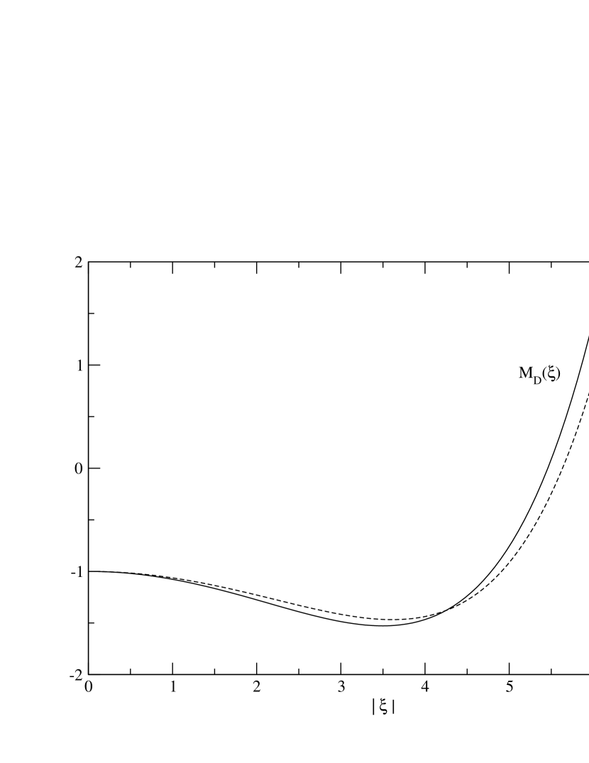
Figure 2: Functions $M_{D}$ and $M_{M}$, corresponding to equation (47) for direct and modified Urca reactions, respectively.

Thus, the relative size of $\eta^{\infty}_{\alpha}$ and $kT_{\infty}$ will determine, through the functions $M_{*}$, whether there is net cooling or heating due to the neutrino emitting reactions. Since the functions $M_{*}$ are even, they do not depend on the sign of the $\xi_{\alpha}$. We plot the functions $M_{*}(\xi)$ for the direct and modified Urca case in Figure 2. With $\xi=0$, the constant term in $F_{*}$ gives the conventional cooling case. As $|\xi|$ grows, the cooling is enhanced by the additional neutrino emission due to the chemical imbalance, reaching a maximum cooling at $|\xi|\sim 3.5$. For larger values of $|\xi|$, the heating becomes important, completely balancing the cooling for $|\xi|\sim 5.5$. For very large values of $|\xi|$, the heating dominates, growing as $\sim\xi^{6}$ and $\sim\xi^{8}$ in the direct and modified Urca case, respectively. In this limit, a fixed fraction of the energy released is emitted as neutrinos, 3/8 and 1/2 for modified and direct Urca, respectively. The remainder stays behind, heating the star.

3.3 Envelope

Since we want to simulate the evolution of a MSP which has finished accretion, we use the fully accreted envelope model of Potekhin et al. (1997) to calculate the effective surface temperature

$$T_{s}^{4}=10^{24}g_{14}\left(1.81e^{-\Phi_{b}}T_{\infty,8}\right)^{2.42}\textrm{K}^{4},$$ (49)

where $g_{14}$ is the surface gravity in units of $10^{14}$ cm s^-2, $T_{\infty,8}$ is the internal temperature in units of $10^{8}$ K, and $\Phi_{b}\equiv\Phi(r_{b})$. The photon luminosity then follows from equation (6). An accreted envelope is more heat transparent than a pure iron one for $T_{s}\gtrsim 10^{5}$ K, leading to faster cooling, whereas for $T_{s}\lesssim 10^{5}$ K the opposite happens (Potekhin et al., 1997).

3.4 Heat Capacity

To calculate the integral in equation (3), we use the specific heat capacities at constant volume $c_{V,i}$ for degenerate, non-superfluid fermions (see, e.g., Levenfish & Yakovlev 1994). In analogy with the neutrino emissivity, we can separate the temperature dependence from the spatial one. From equation (3), we can define

$$\tilde{C}\equiv\frac{C}{T_{\infty}}=\frac{k^{2}}{3\hbar^{3}}\sum_{i}\int 4\pi r^{2}e^{\Lambda}m_{i}^{*}(n)p_{Fi}(n)e^{-\Phi}dr,$$ (50)

where $p_{Fi}$ and $m^{*}_{i}$ are the Fermi momentum and effective mass of species $i$, respectively. The latter can be obtained analytically for the APR and PAL EOSs (see, e.g., Page et al. 2004), while for the noninteracting Fermi gas we use $m^{*}_{i}=\mu_{i}/c^{2}$, where $\mu_{i}$ is the chemical potential of species $i$. The sum is performed over all particle species and the integral is done over the region where each particle species exists. We take only free particles into account, neglecting the heat capacity due to the lattice of ions in the crust.

3.5 Crustal Processes

In this work, we are neglecting processes in the crust which might also modify the total number of neutrons, protons, or electrons. We may ask here if this choice is a good approximation for computing the evolution of the chemical imbalances, since the short diffusion timescale limit means that the chemical equilibrium everywhere in the star can be restored by reactions occurring wherever these are fastest. Iida & Sato (1997) calculated the heating of a neutron star due to spin-down compression in the crust. They found that neutron absorptions in the inner crust are the dominant non-equilibrium process, producing a very small heating rate $H(t)\approx 5\times 10^{-7}\dot{E}$, where $\dot{E}$ is the spin-down power. Although they did not consider neutron diffusion between different layers in the star, and modelled the spin-down compression as a one-dimensional process, we take their result to suggest a very small contribution to the total heating. Since the inner crust accounts for about 2% of the total baryons in the star and the neutrino emissivities of the core overwhelm crustal emission processes, we integrated equations (12) only over the core and neglected processes in the crust, under the assumption that the error introduced would be small. Our results confirm our assumption, since for the more realistic EOSs we obtained heating rates due to core processes much bigger than Iida & Sato’s results (see equation 69). We have to warn that neglecting the crust may not be a good approximation if superfluidity is included, since non-equilibrium processes in the crust can even overtake suppressed Urca reactions in the core. It has also been suggested by Gusakov et al. (2004) that direct Urca reactions could occur at the crust-core interface. We have not explored this possibility. However, we are aware that even a small amount of direct Urca reactions in the inner crust would have a significant effect on the evolution of chemical imbalances.

3.6 Thermal Evolution Equations

Finally, we write the coupled equations for the time evolution of the temperature and the chemical imbalances explicitly for the non-superfluid case with $npe\mu$ composition, taking direct or modified Urca reactions into account. For the internal temperature, from equations (2), (3), (4), (5), (6), (48), and (50), we get

$$\dot{T}_{\infty} = \frac{1}{\tilde{C}}\left[\left(M_{D}(\xi_{npe})\tilde{L}_{De}+M_{D}(\xi_{np\mu})\tilde{L}_{D\mu}\right)T_{\infty}^{5}\right.$$ (51)

$$\left.+\left(M_{M}(\xi_{npe})\tilde{L}_{Me}+M_{M}(\xi_{np\mu})\tilde{L}_{M\mu}\right)T_{\infty}^{7}-L_{\gamma}^{\infty}\right].$$

For the chemical disequilibria, using equations (11), (14), (15), (16), (17), and (30), we obtain

$$\dot{\eta}^{\infty}_{npe} = -\frac{Z_{npe}}{k}\left(\tilde{L}_{De}H_{D}(\xi_{npe})T_{\infty}^{5}+\tilde{L}_{Me}H_{M}(\xi_{npe})T_{\infty}^{7}\right)$$ (52)

$$-\frac{Z_{np}}{k}\left(\tilde{L}_{D\mu}H_{D}(\xi_{np\mu})T_{\infty}^{5}+\tilde{L}_{M\mu}H_{M}(\xi_{np\mu})T_{\infty}^{7}\right)+2W_{npe}\Omega\dot{\Omega},$$

$$\dot{\eta}^{\infty}_{np\mu} = -\frac{Z_{np}}{k}\left(\tilde{L}_{De}H_{D}(\xi_{npe})T_{\infty}^{5}+\tilde{L}_{Me}H_{M}(\xi_{npe})T_{\infty}^{7}\right)$$ (53)

$$-\frac{Z_{np\mu}}{k}\left(\tilde{L}_{D\mu}H_{D}(\xi_{np\mu})T_{\infty}^{5}+\tilde{L}_{M\mu}H_{M}(\xi_{np\mu})T_{\infty}^{7}\right)+2W_{np\mu}\Omega\dot{\Omega},$$

where we have defined

$$Z_{np} = \frac{B_{nn}+B_{np}+B_{pn}+B_{pp}}{B_{nn}B_{pp}-B_{np}B_{pn}},$$ (54)

$$Z_{npe} = \frac{1}{B_{ee}}+Z_{np},$$ (55)

$$Z_{np\mu} = \frac{1}{B_{\mu\mu}}+Z_{np},$$ (56)

and

$$W_{npe} = (Z_{npe}-Z_{np})I_{\Omega,e}+Z_{np}I_{\Omega,p},$$ (57)

$$W_{np\mu} = (Z_{np\mu}-Z_{np})I_{\Omega,\mu}+Z_{np}I_{\Omega,p}.$$ (58)

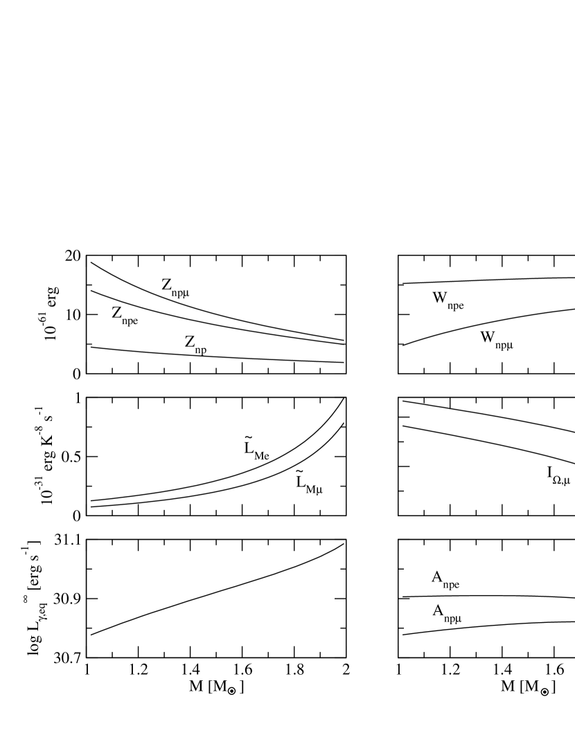
Figure 3: The four higher panels show results for constants defined in section § 3.6, obtained from different stellar models built with the A18 + $\delta\upsilon$ + UIX* EOS. The two lower panels show the dependence on stellar model of the quasi-equilibrium photon luminosity (equation 66) and the constant $A$, assuming $P_{\rm{ms}}=\dot{P}_{-20}=1$ and using the A18 + $\delta\upsilon$ + UIX* EOS. For the latter, the two values are obtained by taking $\ell=npe$ and $\ell=np\mu$ in equation (79), respectively.

Typical values for the different constants are plotted in Figure 3. Since $\Omega\dot{\Omega}<0$, equations (52) and (53) have a positive term, proportional to the spin-down power, which arises from the change in the equilibrium concentrations of each particle species with spin-down and makes the chemical imbalances grow. The remaining terms, opposite in sign to $\eta_{npe}^{\infty}$ and $\eta_{np\mu}^{\infty}$, account for the effect of reactions trying to restore beta equilibrium. Equation (51) has the photon luminosity as a negative term, and the net contribution of neutrino reactions, equation (48), which may be positive or negative depending on the absolute value of $\xi_{npe}$ and $\xi_{np\mu}$. For numerical calculations, the evolution of $\Omega\dot{\Omega}$ was computed assuming magnetic dipole braking with no field decay, relating magnetic field, rotation period, and period derivative by the conventional formula $B\simeq 3.2\times 10^{19}\sqrt{P\dot{P}}$ G, where $P$ is measured in seconds.

4 RESULTS AND DISCUSSION

4.1 Thermal Evolution

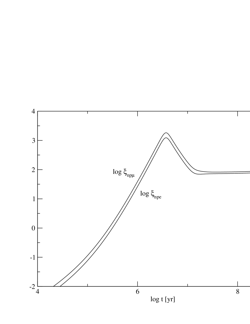
Figure 4: Evolution of the internal temperature and chemical imbalances (left) and the ratios $\xi=\eta^{\infty}/(kT_{\infty})$ (right), for a 1.4$M_{\sun}$ star calculated with the A18 + $\delta\upsilon$ + UIX* EOS, with initial conditions $T_{\infty}=10^{8}$ K and null chemical imbalances at $t=0$, and spin-down parameters $B=10^{8}$ G and $P_{0}=1$ ms.

A typical solution of equations (51), (52), and (53) is shown in the left panel of Figure 4. First, the temperature starts falling as in the conventional cooling case, while the chemical imbalances grow due to spin-down compression. At some point, the ratios $\xi_{npe}$ and $\xi_{np\mu}$ (right panel of Figure 4) are big enough, so that the net contributions of neutrino reactions, equation (48), are positive, and their sum exceeds $L_{\gamma}^{\infty}$. The temperature then starts rising. The chemical imbalances continue to grow, more slowly than the temperature and hence reducing $\xi_{npe}$ and $\xi_{np\mu}$. Finally, the star can arrive at a quasi-equilibrium state, where the rate at which spin-down modifies equilibrium concentrations is the same as the rate at which reactions drive the system towards the equilibrium configuration, with heating and cooling balancing each other (Reisenegger, 1995). The subsequent thermal evolution can then be approximated by the simultaneous solution of the equations $\dot{T}_{\infty}=0$ and $\dot{\eta}_{npe}^{\infty}=\dot{\eta}_{np\mu}^{\infty}=0$. We discuss this quasi-equilibrium solution in detail in §4.2.

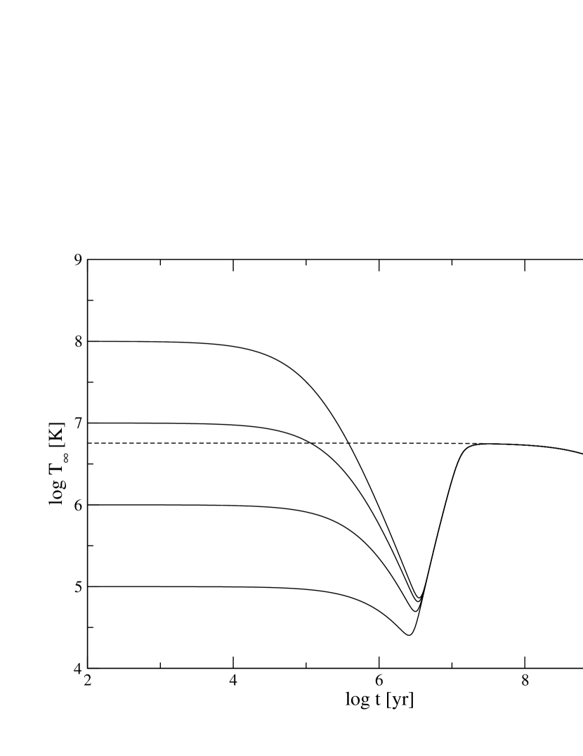
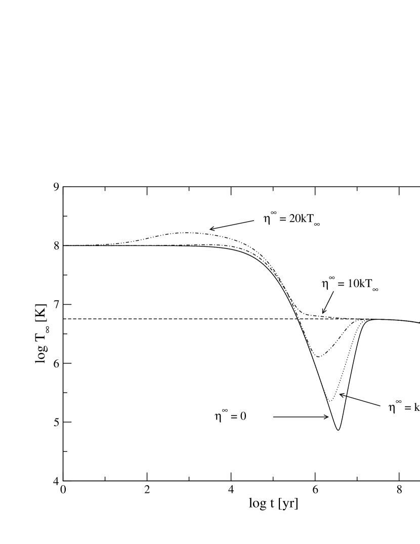
Figure 5: Evolution of the internal temperature for different initial conditions on temperature (left) and chemical imbalances (right). For both plots we set $\eta_{npe}^{\infty}=\eta_{np\mu}^{\infty}\equiv\eta^{\infty}$ at $t=0$. Fixed initial values are $\eta^{\infty}=0$ (left) and $T_{\infty}=10^{8}$ K (right). The short-dashed line is the quasi-equilibrium solution, obtained by solving $\dot{T}_{\infty}=0$ and $\dot{\eta}_{npe}^{\infty}=\dot{\eta}_{np\mu}^{\infty}=0$. The stellar model and spin-down parameters are the same as in Figure 4.

The pure modified Urca case ($\tilde{L}_{De}=\tilde{L}_{D\mu}=0$) is the simplest to analyze. Figure 5 shows the thermal evolution of the same star as in Figure 4, this time with different initial conditions of internal temperature (left) and chemical imbalances (right). The spin-down parameters were chosen so that the arrival at the quasi-equilibrium state is clearly visible, the short-dashed lines being the quasi-equilibrium solutions. We note that, in both cases, the value of the temperature at the quasi-equilibrium state and the time required to arrive do not depend on initial conditions.

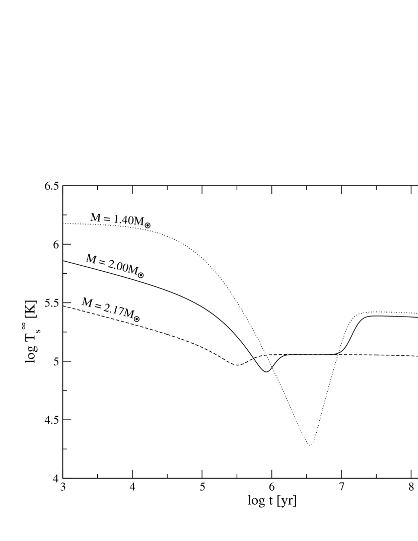
Figure 6: Evolution of surface temperature for different stellar models, calculated using the A18 + $\delta\upsilon$ + UIX* EOS, with fixed initial conditions. The mass of each configuration is labelled on each curve. The 2$M_{\sun}$ star is slightly above the threshold for direct Urca with electrons, but below the threshold for muon direct Urca. The 2.17$M_{\sun}$ star is near the maximum-mass non-rotating configuration, and has direct Urca with electrons and muons. The spin-down parameters are the same as in Figure 4.

If direct Urca reactions are open, solutions change noticeably. In Figure 6 we show the thermal evolution of three different stellar models built with the same EOS, with identical initial conditions and spin-down parameters. The 1.4$M_{\sun}$ star is the same as that of Figure 5, with only modified Urca reactions in operation. The 2$M_{\sun}$ star has electron direct Urca operating, with the corresponding muon reaction forbidden. We see that the minimum temperature is higher and occurs at a much earlier time, after which the system reaches a “metastable” quasi-equilibrium state, corresponding to partial equilibration between $T_{\infty}$ and $\eta^{\infty}_{npe}$. However, $\eta^{\infty}_{np\mu}$ continues to grow, leading the system to a final quasi-equilibrium state, determined by muon modified Urca. The 2.17$M_{\sun}$ star has direct Urca with electrons and muons. This time the final quasi-equilibrium state occurs even earlier than the “metastable” quasi-equilibrium of the 2$M_{\sun}$ star, with the temperature at about the same level.

4.2 The Quasi-Equilibrium State

When only modified Urca reactions operate, it is possible to solve analytically for the quasi-equilibrium values of the photon luminosity $L_{\gamma,eq}^{\infty}$ and chemical imbalances $\eta_{npe,eq}^{\infty}$ and $\eta_{np\mu,eq}^{\infty}$, as function of stellar model and current value of $\Omega\dot{\Omega}$. What makes these approximations possible is the high value of $\xi_{npe}$ and $\xi_{np\mu}$ at quasi-equilibrium. From the right panel of Figure 4, we see that, at quasi-equilibrium ($t\sim 10^{7.5}$ yr), $\xi_{npe}\sim\xi_{np\mu}\sim 200$. This enables us to ignore all but the greatest power in the functions $H_{M}$ and $M_{M}$ (equations 36, 37, and 47):

$$H_{M}(x) \simeq \frac{24}{11513\pi^{8}}x^{7}\equiv C_{H}x^{7}$$ (59)

$$M_{M}(x) \simeq \frac{15}{11513\pi^{8}}x^{8}\equiv C_{M}x^{8}.$$ (60)

The error in this approximation, for $x\sim 200$, is less than one part in 100.

To solve for $L_{\gamma,eq}^{\infty}$, we set $\dot{T}_{\infty}=\dot{\eta}^{\infty}_{npe}=\dot{\eta}^{\infty}_{np\mu}=0$ and use equations (59) and (60) to rewrite (51), (52), and (53) as

$$\tilde{L}_{Me}(\eta_{npe,eq}^{\infty})^{8}+\tilde{L}_{M\mu}(\eta_{np\mu,eq}^{\infty})^{8} = k^{8}L_{\gamma}^{\infty}/C_{M}$$ (61)

$$Z_{npe}\tilde{L}_{Me}(\eta_{npe,eq}^{\infty})^{7}+Z_{np}\tilde{L}_{M\mu}(\eta_{np\mu,eq}^{\infty})^{7} = \frac{2k^{8}}{C_{H}}W_{npe}\Omega\dot{\Omega}$$ (62)

$$Z_{np}\tilde{L}_{Me}(\eta_{npe,eq}^{\infty})^{7}+Z_{np\mu}\tilde{L}_{M\mu}(\eta_{np\mu,eq}^{\infty})^{7} = \frac{2k^{8}}{C_{H}}W_{np\mu}\Omega\dot{\Omega}$$ (63)

Solving for $\eta_{npe,eq}^{\infty}$ and $\eta_{np\mu,eq}^{\infty}$ in equations (62) and (63), we get

$$\eta_{npe,eq}^{\infty}=k\left(\frac{2kI_{\Omega,e}}{C_{H}\tilde{L}_{Me}}\right)^{1/7}(\Omega\dot{\Omega})^{1/7}$$ (64)

$$\eta_{np\mu,eq}^{\infty}=k\left(\frac{2kI_{\Omega,\mu}}{C_{H}\tilde{L}_{M\mu}}\right)^{1/7}(\Omega\dot{\Omega})^{1/7}$$ (65)

where we have used equations (57) and (58) and the fact that $I_{\Omega,p}=I_{\Omega,e}+I_{\Omega,\mu}$. Both chemical imbalances at quasi-equilibrium are positive, since $\Omega\dot{\Omega}$ and $I_{\Omega,i}$ are negative. We finally replace equations (64) and (65) in (61), to obtain the photon luminosity:

$$L_{\gamma,eq}^{\infty}=C_{M}\left(\frac{2k}{C_{H}}\right)^{8/7}\left[\left(\frac{I^{8}_{\Omega,e}}{\tilde{L}_{Me}}\right)^{1/7}+\left(\frac{I^{8}_{\Omega,\mu}}{\tilde{L}_{M\mu}}\right)^{1/7}\right]|\Omega\dot{\Omega}|^{8/7}.$$ (66)

An interesting feature of equation (66) is that it does not depend on envelope model. The reason is that the limit $\eta^{\infty}\gg kT_{\infty}$ implies that reactions are completely determined by chemical imbalances, eliminating any dependence on internal temperature. The energy released is divided in fixed fractions between neutrino emission ($1-[C_{M}/C_{H}]=3/8$) and heating ($C_{M}/C_{H}=5/8$), the latter being radiated entirely as photons. Note also that the ratio $\eta_{npe,eq}^{\infty}/\eta_{np\mu,eq}^{\infty}$ depends only on EOS and stellar model, and is of order unity, thus we will make reference to either of them as $\eta^{\infty}_{\ell}$.

For the entire range of EOSs and stellar models, we can write

$$L_{\gamma,eq}^{\infty}\simeq 10^{30-31}\left(\frac{\dot{P}_{-20}}{P_{\rm{ms}}^{3}}\right)^{8/7}\textrm{erg s}^{-1},$$ (67)

where $\dot{P}_{-20}$ is the period derivative measured in units of $10^{-20}$, and $P_{\rm{ms}}$ the period in ms. Values for different stellar models built with the A18 + $\delta\upsilon$ + UIX* EOS are shown in Figure 3. Using equation (6), we can rewrite equation (67) in terms of the effective temperature:

$$T_{s,eq}^{\infty}\simeq\left(2-3\right)\times 10^{5}\left(\frac{\dot{P}_{-20}}{P_{\rm{ms}}^{3}}\right)^{2/7}\textrm{K}.$$ (68)

This time, the uncertainty due to EOS and stellar model is smaller than 25%. We can also write the ratio of quasi-equilibrium photon luminosity (and thus total heating rate) to the spin-down power $\dot{E}$

$$\frac{L_{\gamma,eq}^{\infty}}{\dot{E}}\sim(0.3-3)\times 10^{-5}\left(\frac{\dot{P}_{-20}}{P_{\rm{ms}}^{3}}\right)^{1/7}.$$ (69)

It is also possible to calculate $\xi_{\ell,eq}$ for the quasi-equilibrium state. Its spin-down power dependence,

$$\xi_{\ell,eq}\propto|\Omega\dot{\Omega}|^{(\alpha-8)/(7\alpha)},$$ (70)

where $\alpha=2.42$ is the exponent of the envelope model of Potekhin et al. (1997) (see §3.3), shows that increasing $|\Omega\dot{\Omega}|$ reduces $\xi_{\ell}$, decreasing the accuracy of the analytical approximation, although very slowly.

4.3 Effect of Hyperons

Although we did not include hyperons in our calculations, we may ask how their presence could modify the thermal evolution. The first particles to appear after muons are probably the $\Sigma^{-}$ and $\Lambda^{0}$ hyperons, which require the introduction of two additional chemical imbalances:

$$\eta_{nn\Sigma p} = 2\mu_{n}-\mu_{\Sigma}-\mu_{p},$$ (71)

$$\eta_{n\Lambda} = \mu_{n}-\mu_{\Lambda}.$$ (72)

Once hyperons are present, the following non-leptonic reactions are open (e.g., Langer & Cameron 1969):

$$n+n \rightleftharpoons \Sigma^{-}+p,$$ (73)

$$n+\Lambda^{0} \rightleftharpoons \Sigma^{-}+p.$$ (74)

Reaction (73) proceeds via weak interactions, since it does not conserve strangeness, while (74) proceeds via strong interactions. Both reactions have timescales several orders of magnitude shorter than beta processes (Langer & Cameron, 1969). Therefore, imbalances (71) and (72) remain small compared to $\eta_{npe}$ and $\eta_{np\mu}$, and reactions (73) and (74) contribute negligibly to the total heat generation. Moreover, since chemical imbalances associated to direct or modified Urca reactions with hyperons are linear combinations of $\eta_{nn\Sigma p}$, $\eta_{n\Lambda}$, $\eta_{npe}$, and $\eta_{np\mu}$, the latter two will determine the heat generation through both nucleon and hyperon reactions.

In order to assess the importance of including the Urca processes involving hyperons in addition to the nucleon processes, consider, as an example, the $\Sigma^{-}$ direct Urca reactions

$$\Sigma^{-}\to n+e+\bar{\nu}_{e},\qquad n+e\to\Sigma^{-}+\bar{\nu}_{e},$$ (75)

whose associated chemical imbalance is $\eta_{\Sigma ne}=\eta_{npe}-\eta_{nn\Sigma p}\approx\eta_{npe}$. Their net effect on equations (52) and (53) is to enhance the electron direct Urca rate according to $\tilde{L}_{De}^{\prime}=\tilde{L}_{De}+\tilde{L}_{\Sigma ne}$, reducing the chemical imbalance and thus the stellar surface temperature. This correction is small, since direct Urca reactions with hyperons are at least a factor 5 weaker than their nucleon analogs (Prakash et al., 1992). For the pure modified Urca case, it can be checked from equation (66) that the correction to the surface temperature introduced by adding several reactions involving hyperons is a factor $[\tilde{L_{n}}/(\tilde{L}_{n}+\tilde{L}_{h})]^{1/28}$, where $\tilde{L}_{n}$ and $\tilde{L}_{h}$ are the nucleon and hyperon Urca luminosities, respectively. Thus, the corrections due to hyperons in a purely modified Urca or purely direct Urca scenario are fairly negligible.

The only important effect of hyperons in the context of rotochemical heating is that, in their presence, conditions for direct Urca processes may become more easily satisfied, as is the case with reactions involving $\Lambda^{0}$ (Prakash et al., 1992). The steep increase of the proton concentration with the appearance of $\Sigma^{-}$ hyperons (e.g., Glendenning 1997) can also cause the condition for nucleon direct Urca to be satisfied at lower densities than if hyperons are excluded from the models.

4.4 Conditions for Arrival at the Quasi-Equilibrium State

We may now ask which of the known MSPs are likely to be in the quasi-equilibrium state. To answer this question, we need to know how long it takes to arrive at the quasi-equilibrium state, and if real pulsars are older than this time. Since the negative “equilibration” terms due to reactions in equations (52) and (53) are important only for imbalances near their equilibrium values (recall the limit $\xi_{\ell}\gg 1$), we can assume that the initial evolution of $\eta^{\infty}_{\ell}$ is due only to $\Omega\dot{\Omega}$:

$$\dot{\eta}^{\infty}_{\ell}\approx 2W_{\ell}\Omega\dot{\Omega}.$$ (76)

Integrating over time, we get

$$\eta_{\ell}^{\infty}(t)\approx|W_{\ell}|\left[\Omega^{2}_{0}-\Omega^{2}(t)\right].$$ (77)

For the true solution to have reached the quasi-equilibrium state, this approximate solution must exceed $\eta_{\ell,eq}^{\infty}(\Omega\dot{\Omega})$. Using equations (64) or (65), together with equation (77), we may express this condition as an upper limit on the initial spin period

$$P_{0}<\frac{P}{\sqrt{1+A}}\equiv P_{0}^{qe},$$ (78)

with

$$A=\frac{1}{|W_{\ell}|}\left(\frac{2k^{8}I_{\Omega,\ell}}{C_{H}\tilde{L}_{\ell}}\right)^{1/7}\frac{(\Omega\dot{\Omega})^{1/7}}{\Omega^{2}}.$$ (79)

(Here and in the rest of this subsection, we assume that only modified Urca processes are active.) Given the current spin parameters of a pulsar, condition (78) gives the highest initial period it can have had, so that enough time has elapsed for it to have reached the quasi-equilibrium state. For MSPs, the constant $A$ is generally small. For a 1.4$M_{\sun}$ star built with the A18 + $\delta\upsilon$ + UIX* EOS, we get

$$A\approx 0.01(\dot{P}_{-20}P_{\rm{ms}}^{11})^{1/7}.$$ (80)

Values for other stellar masses are shown in Figure 3. From equation (76), we can estimate a characteristic timescale for equilibration as

$$\tau_{eq}\sim\frac{\eta^{\infty}_{\ell,eq}}{2W_{\ell}\Omega\dot{\Omega}}=1.6\times 10^{7}\left(P_{\rm{ms}}^{3}\over\dot{P}_{-20}\right)^{6/7}{\rm yr}.$$ (81)

Reisenegger (1995) calculated the thermal evolution of neutron stars with rotochemical heating for different values of the magnetic field, using the magnetic dipole braking model with no field decay. His conclusion was that a necessary condition for the quasi-equilibrium solution to be a good approximation to the exact one is that the spin-down timescale has to be longer than that for the growth of chemical imbalances. To quantify this, we estimate the spin-down timescale as the characteristic age,

$$\tau_{sd}=\frac{P}{2\dot{P}}=\frac{\Omega}{2\dot{\Omega}},$$ (82)

and take the ratio of $\tau_{eq}$ to it, getting

$$\frac{\tau_{eq}}{\tau_{sd}}=A.$$ (83)

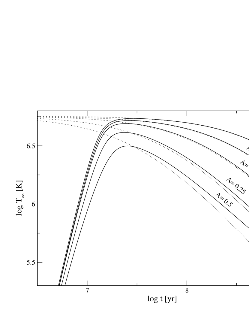
Figure 7: Exact and quasi-equilibrium solutions for the internal temperature of the same star of Figure 4 (solid and dashed lines, respectively), with fixed initial temperature, and different magnetic fields $B$, choosing the initial period $P_{0}$ in each case so as to satisfy $\tau_{eq}=1.5\times 10^{7}$ yr, and therefore implying different initial values of $A$.

Figure 7 shows the internal temperature of our conventional star after the rise from the minimum temperature, for different initial values of $A$, with fixed initial $\tau_{eq}$. Dotted lines are the quasi-equilibrium solutions at the instantaneous value of $\Omega\dot{\Omega}$. The figure suggests that, for high values of $A$, exact and quasi-equilibrium solutions depart from each other, whereas for small $A$, solutions remain “together”. In fact, all solutions depart from each other, the departure being slower with time for smaller $A$. For more general spin-down laws with arbitrary braking index $n=\Omega\ddot{\Omega}/\dot{\Omega}^{2}$, it can be shown analytically that this is true for $1<n<13$. The increase in $\log{(T^{ex}/T^{qe})}$, where $T^{ex}$ is the exact solution and $T^{qe}$ the quasi-equilibrium one, is roughly linear with time. For $A=0.25$ at $t=0$, and assuming a standard braking index $n=3$, $T^{eq}$ is $\sim 5\%$ lower than $T^{ex}$ at $t=\tau_{eq}$, the difference growing 2% every $10^{8}$ yr. Rewriting equation (80) in terms of the magnetic field,

$$A\approx 0.01(P_{\rm{ms}}^{5}B_{8})^{2/7},$$ (84)

where $B_{8}$ is the surface magnetic field in units of $10^{8}$ G, we can easily understand the results of Reisenegger (1995), since increasing $B$ with fixed $P_{0}$ increases the initial value of $A$. Relating $A$ at the present time and at $t=0$ for an arbitrary, but constant, braking index,

$$A(P,\dot{P})=\left(\frac{P}{P_{0}}\right)^{(13-n)/7}A(P_{0},\dot{P}_{0}),$$ (85)

shows that the former is greater than the latter for all reasonable values of $n$. Thus, a small current value of $A$ is a good indicator that the star remains close to the quasi-equilibrium state, as long as it satisfies $P_{0}<P_{0}^{qe}$.

Since constraints on the initial periods $P_{0}^{wd}$ of a few MSPs have been obtained from the cooling ages of their white dwarf companions (Hansen & Phinney, 1998), we can check which objects are likely at the quasi-equilibrium state. In Table Rotochemical Heating in Millisecond Pulsars. Formalism and Non-superfluid case., further discussed in §4.6, we show the range in $P_{0}^{wd}$ for some MSPs obtained by Hansen & Phinney (1998). We made no distinction between the $n=2$ and $n=3$ case, and adopted the widest possible range in $P_{0}^{wd}$. In Table Rotochemical Heating in Millisecond Pulsars. Formalism and Non-superfluid case. we also show the value of $A$ and the upper limit on initial spin period $P_{0}^{qe}$ required for the MSP to be currently in the quasi-equilibrium state. Among MSPs with constraints on initial periods, PSR J1012+5307 is the only one not satisfying the conditions. The small values of $A$ imply that any initial periods substantially shorter than the current ones will leave the MSPs in equilibrium by the present time.

4.5 Predictions for PSR J0437-4715 and PSR J0108-1431

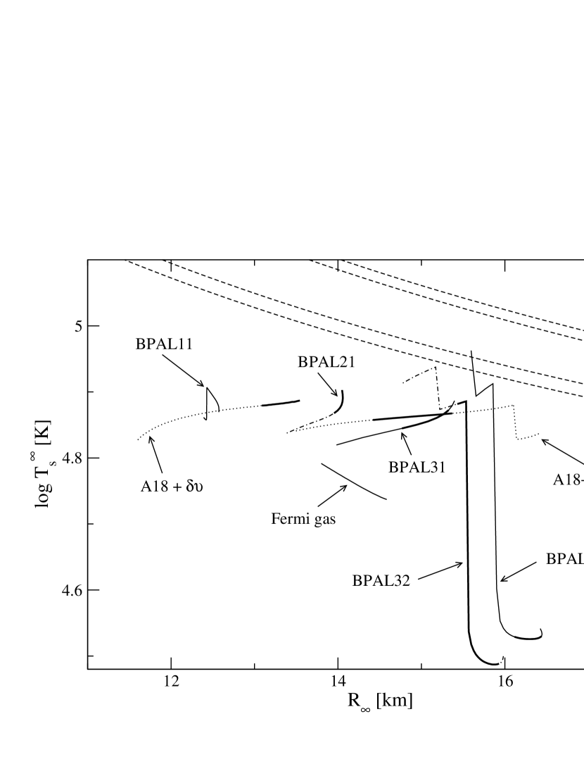
Figure 8: Quasi-equilibrium effective temperatures $T_{s,eq}^{\infty}$ obtained with different EOSs and stellar models, for the spin parameters of PSR J0437-4715. Dashed lines are the 68% and 90% confidence contours of the blackbody fit of Kargaltsev et al. (2004) to probable thermal emission from this pulsar. Bold lines indicate, for each EOS, the range corresponding to the mass constraint of van Straten et al. (2001) for PSR J0437-4715, $M_{PSR}=1.58\pm 0.18M_{\sun}$. Abrupt reductions in temperature with (increasing or decreasing) radius correspond to opening of direct Urca reactions.

Recently, Kargaltsev et al. (2004) measured ultraviolet emission from PSR J0437-4715, the most probable explanation being that it corresponds to thermal radiation. Since this object satisfies $P_{0}^{wd}<P_{0}^{qe}$ with small $A$, we assume that it is already at the quasi-equilibrium state. In Figure 8, we plot the blackbody fit of Kargaltsev et al. (2004) as dashed lines, which correspond to 68% and 90% confidence contours. We overplot our values of $T_{s,eq}^{\infty}$ for the spin parameters of PSR J0437-4715 (van Straten et al., 2001), as function of $R_{\infty}$, for the EOSs listed in Table 1. The bold lines show the range in $R_{\infty}$ corresponding to the mass constraint of van Straten et al. (2001), $M_{PSR}=1.58\pm 0.18M_{\sun}$. The complete mass range for each EOS goes from 1$M_{\sun}$ to 0.95$M_{max}$. The upper limit was chosen to avoid the divergence in the spin-down compression rate for masses near $M_{max}$ (see Figure 1), which makes $T_{s,eq}^{\infty}$ also diverge due to $I_{\Omega,i}$ (see equation 66).

The best agreement with observations is reached if only modified Urca reactions are present. When direct Urca reactions open, there are two abrupt drops in $T_{s,eq}^{\infty}$ with increasing stellar mass, the first one ($\sim 10\%$) due to electron direct Urca, and the second ($\sim 50\%$) due to muon direct Urca. This can be seen in Figure 8 for the curves calculated with BPAL11 and A18 + $\delta\upsilon$ + UIX*, as examples of only electron direct Urca, and in the curves corresponding to BPAL32 and BPAL33, which have electron and muon direct Urca. Perfect agreement could be obtained by allowing masses within $\sim 1\%$ of the maximum-mass non-rotating configuration, for the EOSs with only modified Urca. However, we consider this scenario very unlikely.

Using the EOSs which have only modified Urca reactions within the allowed mass for PSR J0437-4715, we can constrain the predicted effective temperature to the narrow range $T_{s,eq}^{\infty}=(6.9-7.9)\times 10^{4}$ K, about 20% lower than the blackbody fit of Kargaltsev et al. (2004). There are three possible reasons why we are not matching their results:

1. We are not taking superfluidity into account. This would reduce Urca reaction rates, lengthening the equilibration timescale and raising the quasi-equilibrium temperature (Reisenegger, 1997).

2. We are neglecting other heating mechanisms (some of them directly related to superfluidity), which could further raise the temperature at any stage in the thermal evolution. Nonetheless, in MSPs, all proposed mechanisms are less important than rotochemical heating (Schaab et al., 1999).

3. The thermal spectrum could deviate from a blackbody, in the same way as the isolated neutron star RX J1856-3754, which has a well-determined blackbody X-ray spectrum that underpredicts the optical flux (Walter & Matthews, 1997), indicating a more complex spectral shape of its thermal emission.

Kargaltsev and collaborators stress the fact that PSR J0437-4715, despite its much larger spin-down age, has a higher surface temperature than the upper limit for the younger, “classical” pulsar J0108-1431, $T_{s}^{\infty}<8.8\times 10^{4}$ K, inferred from the optical non-detection by Mignani et al. (2003). In this regard, we note that the spin-down power ($\propto\Omega\dot{\Omega}$) of the latter pulsar is 680 times lower than that of J0437, making rotochemical heating substantially less important. Its equilibration timescale, according to equation (81), is $2\times 10^{11}$ yr, longer than the age of the Universe and certainly much longer than the spin-down age of the pulsar. Thus, it is not expected to be even close to reaching its quasi-equilibrium state (although it is old enough to have lost its initial heat content). Its actual temperature should therefore be substantially smaller than the predicted quasi-equilibrium surface temperature, which is already $(680)^{2/7}\approx 6$ times lower than that of J0437, well below the observational upper limit.

4.6 Predictions for other millisecond pulsars

In Table Rotochemical Heating in Millisecond Pulsars. Formalism and Non-superfluid case., we provide predictions of $T_{s,eq}^{\infty}$ (assuming modified Urca reactions and no superfluidity) for several MSPs. Since the high-energy part of their expected thermal spectrum is highly absorbed by neutral hydrogen in the interstellar medium, we chose to order them by decreasing predicted quasi-equilibrium flux in the low-energy (Rayleigh-Jeans) regime,

$$F_{RJ,eq}\propto\frac{T_{s,eq}^{\infty}}{d^{2}},$$ (86)

where $d$ is the distance to the object. Each $F_{RJ,eq}$ entry in Table Rotochemical Heating in Millisecond Pulsars. Formalism and Non-superfluid case. is scaled by the value for PSR J0437-4715. The first group of MSPs after PSR J0437-4715 are nearby, single MSPs, for which $F_{RJ,eq}$ is expected to be larger than for the binary MSPs, for which the initial period has been estimated from their white dwarf companion (see §4.4). We consider the former as the primary targets for observations analogous to those of Kargaltsev et al. (2004). However, even for PSR J0437-4715, the nearest and brightest MSP known to date, the detection of thermal emission is rather difficult, so the observation of other objects of Table Rotochemical Heating in Millisecond Pulsars. Formalism and Non-superfluid case. will be a real challenge. The second group of MSPs are those with estimates for $P_{0}^{wd}$. However, their low fluxes make the detection of their thermal emission impossible for current instruments.

Optical detections are even more daunting than those in the ultraviolet. The extrapolated Rayleigh-Jeans spectrum of PSR J0437-4715 gives magnitudes $U=26.8$, $B=28.1$, and $V=28.5$, which are completely overwhelmed by the white dwarf companion. The most promising single MSPs have about three times lower expected fluxes at Earth, i. e., are another 1.2 magnitudes fainter, beyond the reach of current telescopes.

5 CONCLUSIONS

In this work, we have made an extensive study of the effect of rotochemical heating in non-superfluid millisecond pulsars. We have set up a general formalism for the thermal evolution in the framework of general relativity, which takes the stellar structure fully into account and can be extended to include both superfluidity and exotic particles. A key ingredient in this formalism is the spin-down compression rate based on the slow-rotation approximation of Hartle (1967).

The main consequence of rotochemical heating is the arrival at a quasi-equilibrium state, in which the effective temperature of a neutron star depends only on the current value of the spin-down power. We argue that most of the known MSPs are very likely in the quasi-equilibrium state. If only modified Urca reactions are allowed, the quasi-equilibrium bolometric photon luminosity in the non-superfluid case can be well approximated by

$$L_{\gamma,eq}^{\infty}\simeq 10^{30-31}\left(\frac{\dot{P}_{-20}}{P_{\rm{ms}}^{3}}\right)^{8/7}\textrm{erg s}^{-1},$$ (87)

independent of the neutron star envelope model.

The influence of EOS and stellar model on the quasi-equilibrium state is very weak, the only significant factor being the occurrence of direct Urca reactions. If they are open for both muons and electrons, quasi-equilibrium temperatures are low, as in the conventional cooling case. If they are open only for electrons, the system arrives at a “metastable” quasi-equilibrium, after which it proceeds as if only modified Urca reactions with muons were present. The highest temperatures are reached when all direct Urca reactions are forbidden.

Even our highest predicted quasi-equilibrium effective temperatures are lower than the blackbody fit of Kargaltsev et al. (2004) to the UV emission of PSR J0437-4715 by about 20%. The inclusion of superfluidity will likely raise our predicted temperatures, being the subject of future work.

Appendix A Coincidence of Surfaces of Constant Pressure and Energy Density in General Relativity

In this Appendix, we show that, in uniformly rotating, relativistic stars in hydrostatic equilibrium, composed of a perfect fluid, the surfaces of constant pressure and those of constant energy density coincide, as in the Newtonian case, even if the equation of state is not barotropic. In addition, the gravitational redshift is constant on the same surfaces. This result, together with the diffusive equilibrium condition, allows us to describe the spin-down compression in terms of Lagrangian changes of thermodynamic variables on isobaric surfaces enclosing a fixed baryon number, since all thermodynamical quantities are constant on each isobar. As a by-product, we also provide an alternative derivation of the equation of hydrostatic equilibrium for uniformly rotating, relativistic stars.

The assumption a perfect (i.e., non-dissipative) fluid, whose stress-energy tensor depends only on the energy density $\rho$ and (isotropic) pressure $P$, is of course not strictly true in the astrophysical situation of interest in this paper, in which entropy is generated by non-equilibrium weak interactions, particle diffusion, and heat conduction, and lost (from the star) through the emission of neutrinos and photons. However, the total energy dissipated (and eventually lost) along the star’s lifetime is much smaller than that associated with the mass, random motions, and interactions of its particles, as well as its rotation, and the time scale of the release of this energy is many orders of magnitude longer than the dynamical time and the rotation period of the star. Therefore, the contribution of these dissipative processes to the energy and momentum fluxes is extremely small and can be neglected in the stress-energy tensor. This is in line with the usual approach (also used in neutron star cooling calculations and in the rest of this paper) of neglecting thermal effects when calculating the structure of the star, which is regarded as a fixed background on which thermal processes take place.

The metric of a stationary, axially symmetric system can be written in the form (see, e.g., Hartle 1967):

$$ds^{2}=g_{tt}dt^{2}+g_{rr}dr^{2}+g_{\theta\theta}d\theta^{2}+g_{\phi\phi}d\phi^{2}+2g_{t\phi}dtd\phi,$$ (A1)

where the metric coefficients are functions of $r$ and $\theta$ only. The components of the 4-velocity of any fluid element of the uniformly rotating star are $u^{r}=u^{\theta}=0$, and $u^{\phi}=\Omega u^{t}$, with

$$u^{t}=\left(-\left[g_{tt}+2\Omega g_{t\phi}+\Omega^{2}g_{\phi\phi}\right]\right)^{-1/2}.$$ (A2)

We note that $1/u^{t}$ is the gravitational redshift factor, which corrects the energy of a freely moving particle, as it is measured by observers co-moving with fluid elements on different surfaces inside the star.

The energy-momentum conservation equation can then be written as

$$T^{\alpha\gamma}_{\phantom{\alpha\gamma};\gamma}=(\rho+P)u^{\alpha}_{\phantom{\alpha};\gamma}u^{\gamma}+(\rho+P)u^{\alpha}u^{\gamma}_{\phantom{\gamma};\gamma}+P_{,\gamma}g^{\alpha\gamma}=0,$$ (A3)

where $T^{\alpha\beta}$ are the components of the stress-energy tensor of a perfect fluid. Applying to this equation a projection operator orthogonal to the four-velocity, $\wp_{\alpha\beta}=g_{\alpha\beta}+u_{\alpha}u_{\beta}$ (Schutz, 1985), we get

$$(g_{\alpha\beta}+u_{\alpha}u_{\beta})(\rho+P)u^{\gamma}\Gamma^{\alpha}_{\delta\gamma}u^{\delta}+P_{,\beta}=0.$$ (A4)

Since the only non-vanishing terms are those with $\gamma$ and $\delta$ taking the values $\{t,\phi\}$, the relevant connection coefficients are

$$\Gamma^{\alpha}_{\delta\gamma}=\cases{0,&if $\alpha=t,\phi$;\cr-\frac{1}{2}g^{\alpha\mu}g_{\delta\gamma,\mu},&if $\alpha=r,\theta$.\cr}$$ (A5)

Hence, equation (A3) yields

$$P_{,\beta}-\frac{1}{2}(\rho+P)u^{\gamma}u^{\delta}g_{\delta\gamma,\beta}=0.$$ (A6)

Using equation (A2), we arrive at the equation of hydrostatic equilibrium

$$P_{,\beta}-(\rho+P)(\ln{u^{t}})_{,\beta}=0,$$ (A7)

which is in agreement with the result of Cook, Shapiro & Teukolsky (1992), for the special case of rigid rotation. This shows that the redshift factor $1/u^{t}$ is also constant on the surfaces of constant $P$. Thus, we can write

$$\frac{dP}{d\ln{u^{t}}}=-(\rho+P),$$ (A8)

which implies that $\rho$ is also constant on the same surfaces.

Appendix B Continuity of the Compression Rate across Phase Transitions

In this Appendix, we show that each term of the spin-down compression rate, equation (18), is continuous across a phase transition, even if the energy density and baryon number density change discontinuously. We use units with $G=c=1$.

The discontinuous quantities in the derivative $(dN/dP)_{\Omega^{2},A}$, equation (25), are $n$ and $dP/dr$. The Gibbs free energy per unit volume for $npe\mu$ matter in beta equilibrium at $T=0$ is

$$P+\rho=\mu_{n}n.$$ (B1)

Since, at a phase transition, the pressure $P$ and neutron chemical potential $\mu_{n}$ are continuous, the fractional size of the number density jump can be written as

$$\frac{\Delta n}{n}=\frac{\Delta\rho}{P+\rho}.$$ (B2)

where $\Delta n$ is the positive jump in number density. From the relativistic stellar structure equations, we have

$$\frac{dP}{dr}=-(\rho+P)\frac{M+4\pi r^{3}P}{r(r-2M)}.$$ (B3)

The fractional size of the corresponding jump across the phase transition is

$$\frac{\Delta dP/dr}{dP/dr}=\frac{\Delta\rho}{\rho+P}.$$ (B4)

Thus, from equations (B2) and (B4), we see that the quantity $n/(dP/dr)$ is continuous across a phase transition, and so is $(dN/dP)_{\Omega^{2},A}$.

Regarding the derivative $(dN/d\Omega^{2})_{P,\varepsilon_{0}}$, equation (19), since the jump in $n$ is integrated in equation (21), $N(\rho_{c},P,0)$ is continuous. For $N(\rho_{c},P,\Omega^{2})$, the jump in $n$ due to the last term of equation (24) is cancelled by the contribution from $dn/dr$ in the integral. Using

$$\frac{dn}{dr}=-\Delta n\delta(r-r_{t})+\textrm{continuous part},$$ (B5)

where $\delta$ is Dirac’s delta function and $r_{t}=r(\rho_{c},P_{t})$, with $P_{t}$ the pressure at which the phase transition occurs, we can write

$$-\int_{0}^{r}4\pi y^{2}e^{\Lambda(y)}\xi_{0}(y)\frac{dn}{dy}dy=4\pi r_{t}^{2}e^{\Lambda(r_{t})}\xi_{0}(r_{t})\Delta n\Theta(r-r_{t})+\textrm{continuous part},$$ (B6)

where $\Theta$ is the step function. Equation (B6) is equal to minus the jump (increasing $r$) of the last term in equation (24).

Finally, for the derivative $(dN/d\rho_{c})_{P,\Omega^{2}}$, the contribution from $(\partial n/\partial\rho_{c})_{r}$ to the integral in equation (26) cancels out the discontinuity due to $n$ in the first term. Using

$$\left(\frac{\partial n}{\partial\rho_{c}}\right)_{r} = \frac{r_{i}-r_{t}}{|r_{i}-r_{t}|}\Delta n\delta(\rho_{c}-\rho_{c}^{*})+\textrm{continuous part}$$ (B7)

$$= \frac{r_{i}-r_{t}}{|r_{i}-r_{t}|}\Delta n\bigg{|}\left(\frac{\partial r}{\partial\rho_{c}}\right)_{P}\bigg{|}_{r=r_{t}}\delta(r-r_{t})+\textrm{continuous part},$$

where $P(\rho_{c}^{*},r)=P_{t}$, and $r_{i}(\rho_{c})$ the radial coordinate at which $(\partial n/\partial\rho_{c})_{r}=0$, we can write

$$\int_{0}^{r}4\pi y^{2}e^{\Lambda(y)}\left(\frac{\partial n}{\partial\rho_{c}}\right)_{y}dy=4\pi r_{t}^{2}e^{\Lambda(r_{t})}\frac{(r_{i}-r_{t})}{|r_{i}-r_{t}|}\Delta n\bigg{|}\left(\frac{\partial r}{\partial\rho_{c}}\right)_{P}\bigg{|}_{r=r_{t}}\Theta(r-r_{t})+\textrm{cont. part},$$ (B8)

which is the negative of the jump (increasing $r$) of the first term in equation (26), since the sign of $(\partial r/\partial\varepsilon_{0})_{P}$ is also $(r_{i}-r_{t})/|r_{i}-r_{t}|$.

The right panel of Figure 1 shows the spin-down compression rate inside the core of several stellar models built with the A18 + $\delta\upsilon$ + UIX* EOS, which has a phase transition. The occurrence of the transition can be seen as a (fairly harmless) discontinuity in the derivative of each curve.

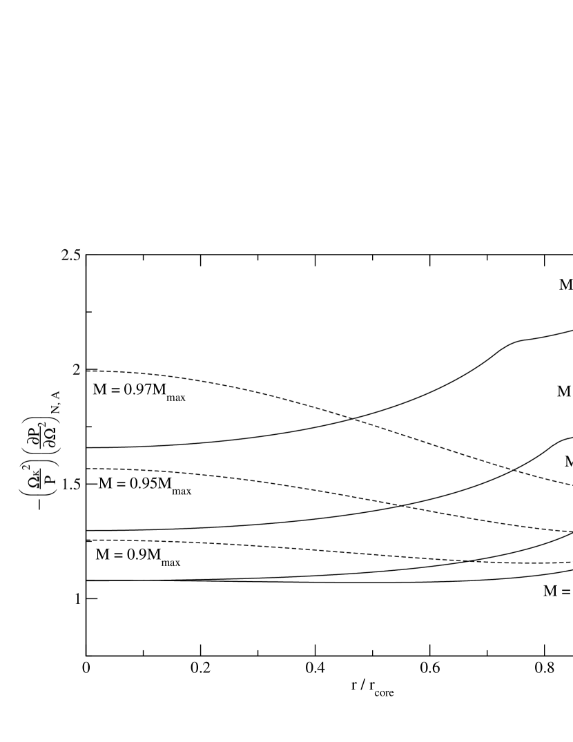
Figure 1: Left: Spin-down compression rate for four different EOSs, normalized by pressure and Kepler frequency. Stellar models have fixed central pressure $P_{0}=4.5\times 10^{34}$ dyn cm^-2. Right: Fractional compression for different stellar models built with the A18 + $\delta\upsilon$ + UIX* EOS. Stars are labelled by their mass in units of the maximum-mass non-rotating configuration (2.19$M_{\sun}$).

Table 1: Maximum-mass non-rotating configuration and Kepler period for the equations of state used in this paper

EOS	$M_{max}$	$\rho_{c}$	$R$	$R_{\infty}$	$P_{K}$
	($M_{\sun}$)	($10^{15}$ g cm-3)	(km)	(km)	(ms)
A18 + $\delta\upsilon$	1.55	1.86	19.81	13.42	-
A18 + $\delta\upsilon$ + UIX∗	2.19	2.78	19.97	16.79	0.51
BPAL 11	1.42	4.45	18.42	11.86	0.54
BPAL 21	1.70	3.46	19.33	13.69	0.56
BPAL 31	1.91	2.86	10.10	15.18	0.59
BPAL 32	1.95	2.66	10.56	15.64	0.63
BPAL 33	1.97	2.53	10.92	15.94	0.66
Fermi gas	0.62	1.10	12.77	13.80	0.98

Table 2: Predictions for MSPs likely to be observable or with estimates for initial spin period

Object	$P$	$\dot{P}$	$d$	$T_{s,eq}^{\infty}$	$F_{RJ,eq}$	$A$	$P_{0}^{qe}$	$P_{0}^{wd}$	Refs.
	(ms)	($10^{-20}$)	(kpc)	($10^{5}$ K)	($F_{0437,eq})$		(ms)	(ms)
J0437-4715	5.76	1.86	0.14	0.72	1	0.17	5.33	2.4–5.3	1, 2
J1024-0719	5.16	$<$1.85	$<$0.25	$<$0.79	$\sim$ 0.35	$<$0.14	$>$4.82	…	3, 4
J2124-3358	4.93	1.23	0.27	0.74	0.28	0.13	4.64	…	3, 4
J0030+0451	4.87	$<$1.00	0.32	$<$0.70	$<$0.19	$<$0.12	$>$4.60	…	4, 5
J1744-1134	4.07	0.71	0.36	0.74	0.15	0.09	3.90	…	6
B1257+12	6.22	4.26	0.45	0.86	0.12	0.22	5.63	…	3, 4
J0034-0534	1.88	$<$0.67	0.53	$<$1.41	$<$0.14	$<$0.03	$>$1.85	$<$1.4	2, 4, 7
J1012+5307	5.26	1.34	0.41	0.71	0.11	0.14	4.93	$>$5.1	2, 4, 8
B1855+09	5.36	1.74	0.90	0.76	0.03	0.15	5.00	$<$4.6	2, 3, 9
J1713+0747	4.57	0.81	1.10	0.70	0.02	0.11	4.35	2.2–3.1	2, 10
J1640+2224	3.16	0.16	1.15	0.60	0.01	0.05	3.08	$>$1.6	2, 4, 11
J2019+2425	3.93	$<$0.70	1.49	$<$0.76	$<$0.01	$<$0.08	$>$3.87	0.9–3.9	2, 4, 12

References. — (1) van Straten et al. (2001); (2) Hansen & Phinney (1998); (3) Toscano et al. (1999a); (4) Cordes & Lazio (2002); (5) Lommen et al. (2000); (6) Toscano et al. (1999b); (7) Bailes et al. (1994); (8) Lange et al. (2001); (9) Kaspi et al. (1994); (10) Splaver et al. (2004); (11) Wolszczan et al. (2000); (12) Nice et al. (2001).

References

- Akmal et al. (1998) Akmal, A., Pandharipande, V. R., & Ravenhall, D. G. 1998, Phys. Rev. C, 58, 1804
- Backer et al. (1982) Backer, D. C., Kulkarni, S. R., Heiles, C., Davis, M. M., & Gross, W. M. 1982, Nature, 300, 615
- Bailes et al. (1994) Bailes, M., et al. 1994, ApJ, 425, L41 F., Thorsett, S. E., & Kulkarni, S. R. 1994, ApJ, 421, L15
- Cheng et al. (1992) Cheng, K. S., Chau, W. Y., Zhang, J. L., & Chau, H. F. 1992, ApJ, 396, 235
- Cheng & Dai (1996) Cheng, K. S., & Dai, Z. G. 1996, ApJ, 468, 819
- Cook et. al. (1992) Cook, G. B., Shapiro, S. L., & Teukolsky, S. A. 1992, ApJ, 398, 203
- Cordes & Lazio (2002) Cordes, J. M., & Lazio, T. J. W. 2002, preprint (astro-ph/0207156) S., Wolszczan, A., & Camilo, F. 1993, ApJ, 410, L91
- Glendenning (1992) Glendenning, N. K. 1992, Phys. Rev. D, 46, 1274
- Glendenning (1997) Glendenning, N. K. 1997, Compact Stars (New York: Springer)
- Gudmundsson et al. (1983) Gudmundsson, E. H., Pethick, C. J, & Epstein, R. I. 1983, ApJ, 272, 286
- Gusakov et al. (2004) Gusakov, M. E., Yakovlev, D. G., Haensel, P., & Gnedin, O. Y. 2004, A&A, 421, 1143
- Haensel (1992) Haensel, P. 1992, A&A, 262, 131
- Haensel & Pichon (1994) Haensel, P., & Pichon, B. 1994, A&A, 283, 313
- Haensel et al. (1995) Haensel, P., Salgado, M., & Bonazzola, S. 1995, ApJ, 296, 745
- Hansen & Phinney (1998) Hansen, B. M. S., & Phinney, E. S. 1998, MNRAS, 294, 569
- Hartle (1967) Hartle, J. B. 1967, ApJ, 150, 1005
- Hartle & Thorne (1968) Hartle, J. B & Thorne, K. S. 1968, ApJ, 153, 807
- Heiselberg et al. (1993) Heiselberg, H., Pethick, C. J., & Staubo, E. F. 1993, Phys. Rev. Lett., 70, 1355
- Hobbs et al. (2004) Hobbs, G., Manchester, R., Teoh, A., & Hobbs, M. 2004, in IAU Symp. 218, Young Neutron Stars and Their Environments, ed. F. Camilo & B. Gaensler (San Francisco: ASP), 139
- Iida & Sato (1997) Iida, K., & Sato, K. 1997, ApJ, 477, 294
- Kargaltsev et al. (2004) Kargaltsev, O., Pavlov, G. G., & Romani, R. 2004, ApJ, 602, 327
- Kaspi et al. (1994) Kaspi, V. M., Taylor, J. H., & Ryba, M. F. 1994, ApJ, 428, 713
- Khodel et al. (2004) Khodel, V. A., Clark, J. W., Takano, M., & Zverev, M. V. 2004, Phys. Rev. Lett., 93, 151101
- Lange et al. (2001) Lange, Ch., Camilo, F., Wex, N., Kramer, M., Backer, D. C., Lyne, A. G., & Doroshenko, O. 2001, MNRAS, 326, 274
- Langer & Cameron (1969) Langer, W. D., & Cameron, A. G. W. 1969, Ap&SS, 5, 213
- Lasota et al. (1996) Lasota, J. P., Haensel, P., & Abramowicz, M. A. 1996 ApJ, 456, 300
- Levenfish & Yakovlev (1994) Levenfish, K. P. & Yakovlev, D. G. 1994, Astronomy Reports, 38, 247
- Lommen et al. (2000) Lommen, A. N., et al., ApJ, 545, 1007
- Mignani et al. (2003) Mignani, R. P., Manchester, R. N., & Pavlov, G. G. 2003, ApJ, 582, 978
- Misner & Sharp (1964) Misner, C. W., & Sharp, D. H. 1964, Phys. Rev., 136, B571
- Nice et al. (2001) Nice, D. J., Splaver, E. M., & Stairs, I. H. 2001, ApJ, 549, 516
- Oppenheimer & Volkoff (1939) Oppenheimer, J. R., & Volkoff, G. M. 1939, Phys. Rev., 55, 374
- Page et al. (2004) Page, D., Lattimer, J. M., Prakash, M., Steiner, A. W. 2004, ApJS, in press (astro-ph/0403657)
- Pethick et al. (1995) Pethick, C. J., Ravenhall, D. G., & Lorentz, C. P. 1995, Nucl. Phys. A, 584, 675
- Potekhin et al. (1997) Potekhin, A. Y., Chabrier, G., & Yakovlev, D. G. 1997, A&A, 323, 415
- Prakash et al. (1988) Prakash, M., Ainsworth, T. L., & Lattimer, J. M. 1988, Phys. Rev. Lett., 61, 2518
- Prakash et al. (1992) Prakash, M., Prakash, M., Lattimer, J. M., & Pethick, C. J. 1992, ApJ, 390, L77
- Prakash et al. (1997) Prakash, M., Bombaci, I., Prakash, M., Ellis, P. J., Lattimer, J. M., & Knorren, R. 1997, Phys. Rep., 280, 1
- Reisenegger (1995) Reisenegger, A. 1995, ApJ, 442, 749
- Reisenegger (1997) Reisenegger, A. 1997, ApJ, 485, 313
- Schaab et al. (1999) Schaab, Ch., Sedrakian, A., Weber, F., & Weigel, M. K. 1999, A&A, 346, 465
- Schutz (1985) Schutz, B. F. 1985, A first course in general relativity (Cambridge: Cambridge University Press)
- Shapiro & Teukolsky (1983) Shapiro, S. L., & Teukolsky, S. A. 1983, Black Holes, White Dwarfs, and Neutron Stars (New York: Wiley)
- Shibazaki & Lamb (1989) Shibazaki, N., & Lamb, F. K. 1989, ApJ, 346, 808
- Splaver et al. (2004) Splaver, E. M., Nice, D. J., Stairs, I. H., Lommen, A. N., & Backer, D. C. 2004, ApJ, in press (astro-ph/0410488)
- Thorne (1977) Thorne, K. S. 1977, ApJ, 212, 825
- Toscano et al. (1999a) Toscano, et al. 1999a, MNRAS, 307, 925
- Toscano et al. (1999b) Toscano, et al. 1999b, ApJ, 523, L171
- van Straten et al. (2001) van Straten, W., et al. 2001, Nature, 412, 158
- Walter & Matthews (1997) Walter, F. M., & Matthews, L. D., Nature, 389, 358
- Wolszczan et al. (2000) Wolszczan, A., et al. 2000, ApJ, 528, 907
- Yakovlev et al. (2001) Yakovlev, D. G., et al. 2001, Phys. Rep., 354, 1
- Yakovlev & Pethick (2004) Yakovlev, D. G., & Pethick, C. J. 2004, ARA&A, 42, 169